A geodetic study of the Alpine Fault through South Westland: using campaign GPS data to model slip rates on the Alpine Fault

ABSTRACT

Although the Alpine Fault has been studied extensively, there have been few geodetic studies in South Westland. We include a series of new geodetic measurements from sites across the Haast Pass and preliminary results from a recently established network, the Cascade array that extends from the Arawhata River to Lake McKerrow, a region that previously had few geodetic measurements. We compare the slip rates based on models that include both single and double faults, and consider Alpine Fault dips of 55° and near vertical. Our preferred solution models the Alpine Fault as an infinitely long fault, dipping at 55° with a second (proxy) fault to account for (inboard) distributed deformation. This gives results that are consistent with the Alpine Fault being a predominantly strike-slip fault with a slip rate of 30 ± 2 mm/yr and therefore demonstrates that the slip rate of the Alpine Fault is constant along strike. The locking depth for the fault in this region is c. 17 km. Assuming a near vertical dip angle results in unrealistic high slip rates.

KEYWORDS:

• Alpine Fault
• slip rates
• South Westland
• deformation
• GPS

Introduction

Over the last 20 years, the School of Surveying at the University of Otago has established a dense geodetic network extending across the South Island of New Zealand. The network extends from the east coast near Dunedin across Central Otago and the Alpine Fault to the west coast near Haast (Figure 1). This profile, which crosses the Central Otago and South Westland regions, is located in the southern half of the South Island of New Zealand. The eastern half of the profile is dominated by the Otago fault system, which is characterised by actively growing asymmetric anticlines above buried reverse faults (Beanland and Berryman 1989; Jackson et al. 1996; Litchfield and Norris 2000; Litchfield 2001). These structures are periodically active followed by long periods of quiescence when the activity migrates to another structure in the region (Beanland and Berryman 1989; Litchfield and Norris 2000).

Figure 1. Network sites. (

) Continuous GNSS sites, (

) campaign sites and (

) new Cascade array campaign sites. Big Bay profile sites have black borders (see profiles G and H) using sites south of Martyr River (Table 2, Models G and H).

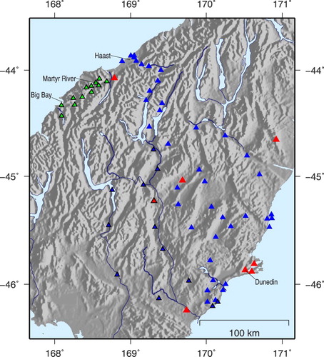
Farther west, the tectonics are dominated by the plate boundary zone where, in the central South Island, the boundary takes up oblique convergence that transitions in the southwestern South Island (South Westland to Fiordland) to subduction of the Australian Plate (Wallace et al. 2007). Barth et al. (2013) identify Martyr River as the change point between the central and southern Alpine Fault. North of Martyr River the plate motion is accommodated as oblique strike-slip (strike 55°, dipping southeast c. 45°), whereas south the motion is almost pure strike-slip and the Alpine Fault becomes nearly vertical (strike 52°, dipping southeast c. 82°) (Barth et al. 2013, Table 1). The vertical component also changes at this point such that the Pacific Plate is uplifting north of the Martyr River and the Australian Plate is uplifting to the south.

Table 1. Model parameters for the single- and double-fault models estimated using both the pre- and post-Dusky Sound 2009 (DS2009) velocity fields. Note that a positive slip rate implies dextral motion. The dip of the Alpine Fault is assumed to be 55° and the antithetic fault is assumed to be 46°.

Fault model		Fault(s)	Strike slip rate		Locking depth
			mm/yr	± 1σ mm/yr	km	± 1σ km
A	Pre-DS2009
	Alpine Fault	1	35.0	0.4	21	1
B	Pre-DS2009
	Alpine Fault	2	30.0	1.5	17	1
	Antithetic fault		4.2	1.0	17	Assumed
C	Post-DS2009
	Alpine Fault	1	37.1	0.8	11	2
H	Post-DS2009	1	36.8	0.2	20 fixed	Assumed
	Alpine Fault (Big Bay profile)

This region has been the subject of geodetic investigations since the 1980s (Blick 1986; Pearson 1990) that were based on the analysis of triangulation measurements, but subject to large measurement errors. The advent of satellite geodesy resulted in improved measurement precision that enabled studies such as Pearson et al. (2000) to examine slip rates on the Alpine Fault with a best fit model that accommodates c. 75% of the relative plate motion and a locking depth of c. 10 km. For the central South Island, Beavan et al. (1999) showed that the majority of the observed velocity signal (50–70%) is uniform slip along strike of the Southern Alps with a shallower locking depth of 5–8 km, which is consistent with higher crustal temperatures associated with a thinner crust. On the eastern side of the Southern Alps and away from the Alpine Fault, Denys et al. (2014, 2016) showed the spatial variation in strain accumulation within the Otago fault system.

In addition to the Otago geodetic data (Denys et al. 2014, 2016), this study includes recent geodetic measurements from sites across the Haast Pass that have not been measured for many years and data from a recently established network, the Cascade array that extends from the Arawhata River to Lake McKerrow, a region that previously had very few geodetic measurements. Together, these data form a broad profile between Dunedin to Haast, and south of Jackson Bay (Figure 1).

Campaign GPS

Our study incorporates campaign and continuous measurements collected over the past 20 years. These data have been observed using traditional GPS methods: tripod, tribrach and antenna set up on traditional surveying marks, typically stainless pins with centring holes grouted into rock or set in concrete. Nominally observing sessions are 2 days (48 h) long, although some of the earlier campaigns were observed with sessions of < 24 h. Although this method is versatile and expedient, it is prone to centring and antenna height measurement errors. The use of different equipment (e.g. antenna) between campaigns, can result in positional errors. This is particularly true for the early measurements in the 1990s when the antenna phase centre models were significantly less accurate than for more modern antenna.

To overcome the centring and antenna height error inherent in traditional GPS campaigns, we have established two networks composed of force-centred marks. In these networks, each antenna is connected to a fixed height adaptor that is attached directly to a 5/8″ threaded rod epoxied into rock. The height of the antenna reference point above the ground depends on the length of the fixed height adaptor and would generally range between 0.055 and 0.15 m. Secure sites are chosen so that equipment can be left unattended for long periods. The two networks containing force-centred points are the Cascade array consisting of marks epoxied into rock outcrops located on ridge tops above the bush line. The array, which was established in 2012, is accessible only by helicopter and observed at c. 1-year intervals between 2013 and 2016. The Central Otago network is similar to the Cascade array except that the marks were developed so that each site had easy, all-weather access (two-wheeled drive vehicle) as well as being secure so that the equipment could be left unattended. The first sequence of Central Otago marks was established in 2004, a second phase in late 2005 and a third phase in 2009. The mark distribution is governed by the layout of the road network, which in turn tends to follow the valleys and basins of the region. This allows for easy and fast access to the marks, but results in the mark distribution being biased towards lower elevations. The surveys have been conducted using a reasonably consistent set of equipment. All measurements since 2004 have used Trimble 5700, R7 and R10 receivers and Trimble Geodetic, Trimble Geodetic 2 or R10 antennas.

GPS processing

GPS data have been processed using the Bernese software package (v. 5.2) (Dach et al. 2015) using 24 h daily position solutions. The Centre for Orbit Determination (CODE) precise satellite orbit and clock parameters, together with the I08.ATX absolute GPS receiver and satellite antenna phase centre model (Schmid et al. 2007) are used to generate daily position time series. The carrier phase ionosphere-free linear combination is used to correct the first-order ionosphere. Higher-order ionospheric effects are not considered here because Hernández-Pajares et al. (2007) and Petrie et al. (2010) showed that these effects are < 1 mm. Tropospheric effects are modelled using the Global Mapping Function, which maps the zenith troposphere delay to the elevation of each observation (Boehm et al. 2007). A 10° elevation cut-off angle is used, a compromise to constrain tropospheric effects but minimise multipath errors. Non-tidal atmospheric loading displacements are modelled according to Ray and Ponte (2003). The effects of ocean loading are corrected using the FES2004 model (Lyard et al. 2006) from the Onsala Space Observatory (holt.oso.chalmers.se/loading). Ambiguity resolution involves a recursive strategy that includes code and phase-based wide lane, QIF and direct L1/L2 fixed ambiguities, depending upon baseline length. The ITRF2014 reference frame is realised through the Helmert three-parameter transformation of the daily coordinate positions. Global IGS sites include those on the stable Pacific, Antarctic and Australian plates. Data outliers were removed using the Median Absolute Deviation (MAD) robust estimator at the 4σ level with σ = 1.4826 × MAD.

Velocity estimation

We model the site position time series assuming linear velocities. Hence the basic equation is:(1) where is the position (ordinate) (m) at time (yr), is the reference position (m) at reference time and is the site velocity (m/yr). The M_W 7.8 Dusky Sound 2009 earthquake (Beavan et al. 2010) not only caused earth displacement at the time of the event throughout the lower South Island (Crook and Donnelly 2013), but also resulted in a new velocity field since the time of the event. Equation (1) is modified to include transient velocity events that act as a time dependent offset (i.e. ramp) with:(2) where is a coseismic offset (m), is the transient velocity (m/yr), is the start time and is the end time of the velocity event ( may be the end of the time series if the velocity change is ongoing as is the case for the Dusky Sound post-seismic relaxation) and is the number of events.

In the case of the continuous GNSS sites where the position time series are estimated daily, the post-seismic deformation is modelled as a characteristic log decay. Following Denys and Pearson (2015, 2016), we model this displacement by modifying Equation (1) such that:(3) where is the coseismic offset (m), is the amplitude of the post-seismic decay (m), is the decay time scale (yr), the event time (yr) and is the number of events. Modelling of seasonal effects (annual and semi-annual cyclic terms) and including any position offsets caused by equipment changes (e.g. replacement antennas) is also included in the continuous position time series (see Denys and Pearson 2015, 2016 for details).

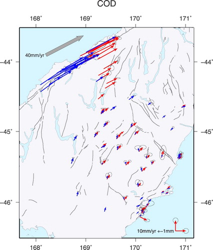
Figure 2 shows the velocity vectors in a Pacific Plate fixed frame after removing the MORVEL (Pacific) plate motion (DeMets et al. 2010). The velocity vectors are generally consistent at the few millimetre level on the east coast, but increase rapidly towards the Alpine Fault. As noted by Sutherland et al. (2006), the vectors in this region are close to being parallel to the trace of the Alpine Fault, which would imply that the fault is predominantly strike-slip.

Figure 2. Site velocities relative to the MORVEL Pacific Plate pole (DeMets et al. 2010). (

) Pre-Dusky Sound 2009 earthquake velocities and (

) post-Dusky Sound 2009 velocities. Error ellipses are shown as 95% confidence intervals.

Modelling infinite faults

We model the fault parallel and normal velocity profiles using equations for infinite faults developed by Savage (1983) and similar to the procedure described by Beavan et al. (1999) and Pearson et al. (2000). We assume uniformity along the fault, thus reducing the problem to two dimensions. This simple but effective model assumes a locking depth below which the fault slips freely at a uniform slip rate. In this case, the plate boundary parallel component of velocity, , is:where is the slip-rate offset (mm/yr), is the slip rate (mm/yr), is the perpendicular distance from the fault (km), is the locking depth of the fault (km) and is the dip of the fault (°). (There is a similar equation for the plate boundary normal component of the velocity field, , however we have included only the plate boundary parallel component in our modelling because the velocity vectors shown in Figure 2 indicate that this portion of the Alpine Fault is predominately strike-slip.)

As a first step towards a tectonic interpretation of the velocity field, we follow the procedure outlined by Pearson et al. (2000) and constructed profiles of the fault parallel and fault normal components of the velocity as a function of distance from the Alpine Fault. We inverted the velocity data to obtain fault slip rates by linearising Equation (4) which models slip on infinite faults (Savage 1983) and use standard least square techniques to find a solution that minimised the sum-squared of the weighted residuals.

Applying this technique requires that the geometry of the Alpine Fault is known. Our study area is located in the transition zone between double-fault geometries; namely, the northern section extending from Haast to Arthur’s Pass (central South Island), where the fault has a dip of c. 50° (Sibson et al. 1979; Norris and Cooper 2001), and the southern section (South Westland) where the Alpine Fault has a nearly vertical dip (Sutherland and Norris 1995; Barth et al. 2013). Although the surface dip of the Alpine Fault is well established by geological studies, the dip of the plate interface at depth is controversial. For example, Lamb and Smith (2013) model the Alpine Fault/Puysegur subduction zone as having a fairly consistent dip of c. 50°. We explored the effect of differing fault geometries by developing profiles with fault dip of between 45° and 80°. Our preferred fault dip is 55° based on the geological evidence from Barth et al. (2013) showing that the dip of the Alpine Fault steepens in our study area.

Results

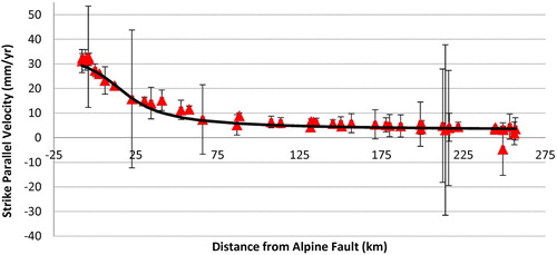
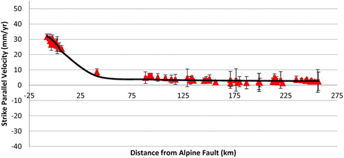
Denys et al. (2016) showed that there is a significant change in the secular velocity field in Central Otago due to the 2009 Dusky Sound earthquake. For this reason, we analysed the pre- and post-earthquake velocities separately. We first inverted the pre-earthquake data by considering the straightforward single-fault model in which all deformation is assumed to be slip on the Alpine Fault. The fault-parallel component of motion is shown in Figure 3 and the model parameters are summarised in Table 1 (Model A). The single-fault model with a dip of 55° is a reasonable fit except that the predicted fault-parallel profile is systematically too low in the range 30–60 km, resulting in a standard error of unit weight (SEUW) of 1.9. This systematic difference is likely to indicate the influence of distributed deformation and/or other unmodelled faults.

Figure 3. Single-fault parallel component of the velocity field based on the pre-Dusky Sound 2009 velocities (Model A). The solid line shows predicted velocity for an infinite Alpine Fault. Triangles represent observed velocities and error bars are at the 1σ level. The x-axis shows distance from the surface trace of the Alpine Fault in km.

Previous studies (Beavan et al. 1999; Pearson et al. 2000) suggest that this extra deformation can be modelled as a second structure running parallel to the Alpine Fault but dipping to the west. Using a block model, Wallace et al. (2007) also showed that the fit of the GPS data improved with a discrete boundary c. 150 km east of the Alpine Fault that accommodated c. 3–4 mm/yr of deformation. Alternatively, the extra deformation could be ascribed to distributed deformation within the Southern Alps. Following Pearson et al. (2000), we modelled the profile with two oppositely dipping shear zones, one of which is identified as the Alpine Fault , whereas the second, west-dipping fault is located c. 150 km east of the Alpine Fault as a proxy for distributed deformation associated with other structures. Equation (5) illustrates the double-fault model in which the right-hand term is the second fault with dip, , and represents perpendicular distance between the double-faults.

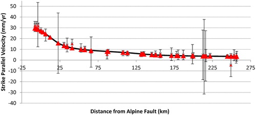
The parameters of our best-fitting double-fault model are listed in Table 1 (Model B), whereas Figure 4 shows the fault-parallel velocities. Incorporating the second fault plane 150 km east of the Alpine Fault produces an improvement in fit with the SEUW decreasing to 1.6. The locking depth and slip rate of the Alpine Fault from our single-fault model are significantly greater than those from Pearson et al. (2000).

Figure 4. Double-fault parallel component of the velocity field based on the pre-Dusky Sound 2009 velocities (Model B). The solid line shows predicted velocity for an infinite Alpine Fault and a second parallel antithetic fault located 152 km southeast (i.e. inboard). Triangles represent observed velocities and error bars are at the 1σ level. The x-axis shows distance from the surface trace of the Alpine Fault in km.

Figure 5 shows the fault-parallel velocity profile for a single-fault model based on only the post-earthquake velocities (Table 1, Model C). A major difference is the significant gradient of the fault-parallel velocities as a result of the Cascade array measurements. The steepness is not obvious with the more limited data set for the pre-Dusky Sound 2009 velocity field. A second difference between the pre- and post-earthquake profiles is the lack of measurements between 6 and 88 km from the Alpine Fault. Because these data are not available, it is not possible to invert for a two-fault model because it is the data in this region that constrain the second fault.

Figure 5. Single-fault parallel component of the velocity field based on the post-Dusky Sound 2009 velocities (Model C). The solid line shows predicted velocity for an infinite Alpine Fault. Triangles represent observed velocities and error bars are at the 1σ errors.

A comparison of the fault parameters in Table 1 shows that the slip rates are very similar between the single-fault models for the pre- and post-Dusky Sound 2009 earthquake data sets, but the locking depth is clearly much less for the post-Dusky Sound earthquake velocity field. This difference shows the importance of the measurements between 6 and 88 km in controlling the locking depth.

The single-fault models (Models A, C) give slip rates on the Alpine Fault that are slightly higher and locking depths that encompass those of Wallace et al. (2007) of 30 mm/yr and 18 km, respectively. However, the double-fault model (Model B) results in a slip rate and a locking depth that that are comparable. The similarity between the two studies is not surprising because the Wallace et al. (2007) model is dominated by the Alpine Fault in this part of the South Island and therefore is one-dimensional in nature. However, the two studies differ in that our models are constrained by additional GNSS data that were not available to Wallace et al. (2007), particularly in South Westland. Our slip rates are higher than those of Beavan et al. (1999) and Pearson et al. (2000) for the double-fault model, but are quite similar for the strike-slip rates from their single-fault model. The strike-slip rate from our double-fault model (Model B) accommodates c. 75% of the MORVEL relative PA/AU plate motion.

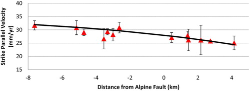
One of the questions that the Cascade array was designed to answer was whether there was any evidence for partial locking on the Alpine Fault. Figure 6 shows the velocity data within ± 10 km of the surface trace of the Alpine Fault. If partial locking was apparent, we would expect to see a discontinuity in the measurements. Because all of the points appear to fit the predicted curve (solid line) within the estimated uncertainties, there does not seem to be any evidence for partial locking at the present time. With more time and measurements, it is expected that the measurement errors will decrease allowing for a more definitive test to be made.

Figure 6. Fault parallel component of the velocity field for the region within 10 km of the surface trace of the Alpine Fault. The solid line shows predicted velocity for an infinite Alpine Fault. Triangles represent observed velocities and error bars are at the 1σ errors.

Our study shows that profiles (Table 2, Models D–F) that assume a vertical (80°) dip for the Alpine Fault provide a good fit to the measured GNSS velocities. Indeed, the profiles are virtually indistinguishable from those shown in Figures 3–6. However, the slip rates from the inversions are significantly higher. Indeed, the resulting slip rates are equal to the total relative plate motion between the Pacific and Australia plates for this part of the plate boundary (40 mm/yr based on the MORVEL plate model, DeMets et al. 2010). These values seem to be unreasonably high, particularly given that other faults are known to be active within Otago, on the inboard or the Pacific Plate side of the Alpine Fault (Beanland and Berryman 1989; Jackson et al. 1996; Litchfield and Norris 2000). For this reason, we prefer the model with the fault dipping at 55°.

Table 2. Model parameters for single and double-fault models estimated using both the pre- and post-Dusky Sound 2009 (DS2009) velocity fields assuming a near vertical Alpine Fault (80° dip) and the antithetic fault is assumed to be 46°.

	Fault model	fault(s)	Strike slip rate		Locking depth
			mm/yr	± 1σ mm/yr	km	± 1σ km
D	Pre-DS2009
	Alpine Fault	1	46.4	0.2	20 fixed	Assumed
E	Pre-DS2009
	Alpine Fault	2	47.6	0.6	20 fixed	Assumed
	Antithetic fault		2.0	0.4	20 fixed	Assumed
F	Post-DS2009
	Alpine Fault	1	47.6	0.5	20 fixed	Assumed
G	Post-DS2009
	Alpine Fault (Big Bay profile)	1	45.7	0.5	20 fixed	Assumed

Barth et al. (2013) suggested that the dip of the Alpine Fault changes along strike in South Westland with the section south of the Martyr River having a near vertical dip. However, it is not clear whether the dip in Barth et al. (2013), which relates to fault geometry in the near surface, is representative of the fault geometry at mid crustal depths. To test this hypothesis, we developed a revised profile centred on Big Bay (44.25°S, 168.05°E, sites with a black border, Figure 1) that incorporates only points south of the Martyr River (Table 2, Model G). Inverting the data gives a slip rate of 46 mm/yr for the Alpine Fault, whereas a profile assuming a dip of 55° (consistent with the rest of the Alpine Fault see Table 1, Model H) gives a slip rate of 37 mm/yr. Note that both these inversions used velocities derived only from post-Dusky Sound 2009 data and in both cases we constrained the locking depth to 20 km because there were insufficient velocity measurements between 10 and 80 km to allow us to invert for this parameter. Also, the model with 55° dip has an SEUW of 1.0 compared with 1.1 for the vertical fault, which indicates that the 55° dipping model has a slightly better fit to the data.

It should be noted that the modelling procedure implicitly assumes an infinite fault without any along strike-slip change in geometry. For this reason, a definitive study of along strike variation in the geometry and locking coefficient will require more sophisticated modelling procedures that have the capability for three-dimensional variation of fault geometry.

Conclusions

The Alpine Fault is a major strike-slip fault that accommodates c. 75% of the current plate motion. It is well recognised that large earthquakes have occurred at regular intervals over geological time making this system important to understand (see e.g. Sutherland et al. 2007). Although the Alpine Fault has been researched extensively, this paper includes new GPS data from South Westland. Because of the effect of the post-seismic deformation from the 2009 Dusky Sound earthquake, the velocity field has been divided into pre- and post-earthquake event data sets. For this broad profile, the Alpine Fault is initially modelled as a single (infinitely long) fault that is uniformly slipping below a (constant) locking depth. Both models have similar strike-slip rates of 37–35 mm/yr respectively. By contrast, the locking depths are significantly different for the two models at 21 km (pre-Dusky Sound 2009 earthquake) and 11 km (post earthquake). However, the models systematically predict lower strike-slip rates that are interpreted to represent distributed deformation to the east of the Alpine Fault.

To account for the (inboard) distributed deformation, a second (proxy) fault is modelled some 150 km east of the Alpine Fault as a double-fault model. The strike-slip rate reduces to 30 mm/yr, with a locking depth of 17 km in this model compared with the single-fault case. Our slip rates are significantly greater than those given by Sutherland et al. (2006). At this stage, the double-fault model can be estimated only using the pre-Dusky Sound velocity field. More GPS measurements are required in the profile between c. 10 and 80 km east of the Alpine Fault.

Our data can also be modelled using a vertical Alpine Fault, however, this model produces slip rates that are greater than the total relative plate motion between the Pacific and Australia plates. For this reason, we prefer a model in which the dip of the Alpine Fault at mid crustal depths is closer to the 50° that characterises the Alpine Fault farther north.

Acknowledgements

Fieldwork support undertaken by Mike Denham and Alastair Neaves (School of Surveying) together with numerous Otago University students. We thank GeoNet (www.geonet.org.nz), the New Zealand Earthquake Commission and Land Information New Zealand (LINZ) for the operation and financial support of the cGNSS network. We thank Laura Wallace, an anonymous reviewer and editor Phaedra Upton for their reviews and useful comments that have improved the quality of this paper.

Disclosure statement

No potential conflict of interest was reported by the authors.

Additional information

Funding

The initial establishment of this Central Otago deformation network was partly funded by an Earthquake Commission grant. The Cascade array was funded through two Otago University research grants. All other GPS data has been funded by NZ Ministry for Science and Innovation (formerly the Foundation for Research, Science and Technology) through the GNS Science New Zealand Geological Hazards and Society Programme (C05X0804) with contributions to the Impacts of Global Plate Tectonics in and around New Zealand Programme (C05X02023).

References

- Barth NC, Boulton C, Carpenter BM, Batt GE, Toy VG. 2013. Slip localization on the southern Alpine fault, New Zealand. Tectonics. 32(3):620–640. doi: 10.1002/tect.20041
- Beanland S, Berryman KR. 1989. Style and episodicity of late Quaternary activity on the Pisa-Grandview fault zone, central Otago, New Zealand. New Zealand Journal of Geology and Geophysics. 32:451–461. doi: 10.1080/00288306.1989.10427553
- Beavan J, Moore M, Pearson C, Henderson M, Parsons B, Bourne S, England P, Walcott D, Blick G, Darby D, Hodgkinson K. 1999. Crustal deformation during 1994–1998 due to oblique continental collision in the central southern Alps, New Zealand, and implications for seismic potential of the Alpine fault. Journal of Geophysical Research: Solid Earth. 104(B11):25233–25255. doi: 10.1029/1999JB900198
- Beavan J, Samsonov K, Denys P, Sutherland R, Palmer N, Denham M. 2010. Oblique slip on the Puysegur subduction interface in the 2009 July MW 7.8 Dusky Sound earthquake from GPS and InSAR observations: implications for the tectonics of southwestern New Zealand. Geophysical Journal International. 183:1265–1286. doi: 10.1111/j.1365-246X.2010.04798.x
- Blick GH. 1986. Geodetic determination of crustal strain from old survey data in Central Otago. In: Reilly WI, Harford BE, editor. Recent crustal movements of the pacific region. Wellington: Royal Society of New Zealand, Bulletin 24; p. 47–54.
- Boehm J, Heinkelmann R, Schuh H. 2007. Short note: a global model of pressure and temperature for geodetic applications. Journal of Geodesy. 81(10):679–683. doi: 10.1007/s00190-007-0135-3
- Crook C, Donnelly N. 2013. Updating the NZGD2000 deformation model, Proceedings of the 125th Annual Conference of the New Zealand Institute of Surveyors (NZIS), August 28–31, 2013; Dunedin, New Zealand.
- Dach R, Lutz S, Walser P, Fridez P. 2015. Bernese GNSS software version 5.2. Bern: Astronomical Institute, University of Bern.
- DeMets C, Gordon RG, Argus DF. 2010. Geologically current plate motions. Geophysical Journal International. 181(1):1–80. doi:10.1111/j.1365-246X.2009.04491.x; see also Erratum, Geophysical Journal International, doi:10.1111/j.1365-246X.2011.05186.x, 2011.
- Denys P, Norris R, Pearson C, Denham M. 2014. A geodetic study of the Otago fault system of the South Island of New Zealand. In: Rizos C, Willis P., editor. Earth on the edge: science for a sustainable planet, international association of geodesy symposia 139. Springer-Verlag Berlin Heidelberg; p. 151–158. doi:10.1007/978-3-642-37222-3_19.
- Denys P, Pearson C. 2015. Modelling time dependent transient deformation in New Zealand. Proceedings of International Symposium on GNSS (IS-GNSS 2015), November 16–19, 2015; Kyoto, Japan.
- Denys P, Pearson C. 2016. Positioning in active deformation zones – implications for NetworkRTK and GNSS processing engines. FIG Working Week 2016, Recovery from Disaster. 2–6 May 2016, Christchurch, New Zealand.
- Denys P, Pearson C, Norris R, Denham M. 2016. A geodetic study of Otago: results of the central Otago deformation network 2004–2014. New Zealand Journal of Geology and Geophysics. 59(1):147–156. doi: 10.1080/00288306.2015.1134592
- Hernández Pajares M, Juan JM, Sanz J, Orús R. 2007. Second order ionospheric term in GPS: implementation and impact on geodetic estimates. Journal of Geophysical Research. 112(B8):921. doi: 10.1029/2006JB004707
- Jackson J, Norris R, Youngson J. 1996. The structural evolution of active fault and fold systems in central Otago, New Zealand: evidence revealed by drainage patterns. Journal of Structural Geology. 18:217–234. doi: 10.1016/S0191-8141(96)80046-0
- Lamb S, Smith E. 2013. The nature of the plate interface and driving force of interseismic deformation in the New Zealand plate-boundary zone, revealed by the continuous GPS velocity field. Journal of Geophysical Research: Solid Earth. 118(6):3160–3189.
- Litchfield NJ. 2001. The titri fault system: Quaternary-active faults near the leading edge of the Otago reverse fault province. New Zealand Journal of Geology and Geophysics. 44:517–534. doi: 10.1080/00288306.2001.9514953
- Litchfield NJ, Norris RJ. 2000. Holocene motion on the Akatore fault, South Otago coast, New Zealand. New Zealand Journal of Geology and Geophysics. 43:405–418. doi: 10.1080/00288306.2000.9514897
- Lyard F, Lefevre F, Letellier T, Francis O. 2006. Modelling the global ocean tides: modern insights from FES2004. Ocean Dynamics. 56(5-6):394–415. doi: 10.1007/s10236-006-0086-x
- Norris RJ, Cooper AF. 2001. Late Quaternary slip rates and slip partitioning on the Alpine fault, New Zealand. Journal of Structural Geology. 23(2):507–520. doi: 10.1016/S0191-8141(00)00122-X
- Pearson C. 1990. Extent and tectonic significance of the Central Otago shear strain anomaly. New Zealand Journal of Geology and Geophysics. 33:295–301. doi: 10.1080/00288306.1990.10425687
- Pearson C, Denys P, Hodgkinson K. 2000. Geodetic constraints on the kinematics of the Alpine fault in the southern South Island of New Zealand, using results from the Hawea-Haast GPS Transect. Geophysical Research Letters. 27(9):1319–1322. doi: 10.1029/1999GL008412
- Petrie EJ, King MA, Moore P, Lavallée DA. 2010. Higher-order ionospheric effects on the GPS reference frame and velocities. Journal of Geophysical Research. 115:B03417. doi:10.1029/2009JB006677.
- Ray RD, Ponte RM. 2003. Barometric tides from ECMWF operational analyses. Annales Geophysicae. 21(8):1897–1910. doi: 10.5194/angeo-21-1897-2003
- Savage J. 1983. Strain accumulation in western United States. Annual Review of Earth and Planetary Sciences. 11(1):11–41. doi: 10.1146/annurev.ea.11.050183.000303
- Schmid R, Steigenberger P, Gendt G, Ge M, Rothacher M. 2007. Generation of a consistent absolute phase-center correction model for GPS receiver and satellite antennas. Journal of Geodesy. 81(12):781–798. doi: 10.1007/s00190-007-0148-y
- Sibson RH, White SH, Atkinson BK. 1979. Fault rock distribution and structure within the Alpine fault zone: a preliminary account. Bulletin of the Royal Society of New Zealand. 18:55–65.
- Sutherland R, Berryman K, Norris R. 2006. Quaternary slip rate and geomorphology of the Alpine fault: implications for kinematics and seismic hazard in southwest New Zealand. Geological Society of America Bulletin. 118(3-4):464–474. doi: 10.1130/B25627.1
- Sutherland R, Eberhart-Phillips D, Harris RA, Stern T, Beavan J, Ellis S, Henrys S, Cox S, Norris RJ, Berryman KR, et al. 2007. Do great earthquakes occur on the Alpine fault in Central South Island, New Zealand? In: Okaya D, Stern T, Davey F, editors. A continental plate boundary: tectonics at South Island, New Zealand. doi:10.1029/175GM12.
- Sutherland R, Norris RJ. 1995. Late Quaternary displacement rate, paleoseismicity, and geomorphic evolution of the Alpine fault: evidence from Hokuri Creek, South Westland, New Zealand. New Zealand Journal of Geology and Geophysics. 38(4):419–430. doi: 10.1080/00288306.1995.9514669
- Wallace LM, Beavan J, McCaffrey R, Berryman K, Denys P. 2007. Balancing the plate motion budget in the South Island, New Zealand using GPS, geological and seismological data. Geophysical Journal International. 168(1):332–352. doi: 10.1111/j.1365-246X.2006.03183.x