A new basin depth map of the fault-bound Wellington CBD based on residual gravity anomalies

ABSTRACT

A new basin depth map for the Wellington Central Business District shows a maximum depth of 540 m near the Wellington Stadium. Our new basin geometry constraints are from a residual gravity anomaly study, based on ∼600 new gravity observations. Residual gravity anomalies are as large as −6.2 mGal with uncertainties <0.1 mGal. Two-dimensional gravity models constrained by boreholes that intersect basement are used to generate the basin depth map. Our maximum depth is twice that previously estimated from other geological and geophysical criteria. An onshore extension of the recently discovered Aotea Fault on the western side of Mt Victoria, is also interpreted from the gravity data. A maximum basement offset of up to 130 m and gravity anomaly gradients up to 8 mGal/km are observed across the fault. A secondary splay off the main Aotea Fault is identified in the NW corner of Mt Victoria, and a possible extension to the Lambton Fault is identified beneath the Wellington Railway Station. This new basin depth and fault trace data provide valuable constraints to models of seismic hazard assessment for Wellington City.

KEYWORDS:

• Sedimentary basins
• earthquake amplification
• earthquake hazard
• gravity anomalies
• basin depth
• fault planes
• basin effects
• Wellington

1. Introduction

Sedimentary basins can create severe, localized amplification of earthquake shaking. This was demonstrated most strikingly by the 1985 M_s 8.1 earthquake in Michoacán, Mexico (McNally et al. 1986) that produced extensive damage and fatalities 400 km away in Mexico City. Similarly, shaking from the 2016 M_w 7.8 Kaikōura earthquake, New Zealand, caused significant damage to mid-rise buildings in Wellington City (Bradley et al. 2017) despite the earthquake being ∼80 km distant (Hamling et al. 2017). Damaging shaking in Wellington City was also noted from the 2013 Cook Strait earthquake (Francois-Holden and Kaiser 2013). Amplification of seismic waves and increased shaking in Wellington City are related to both the thickness of unconsolidated sediment in and the 3D shape of the underlying, fault-bound basin (Benites and Olsen 2005; Bradley et al. 2018).

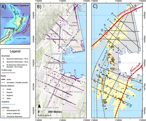
Three dimensional site amplification effects are not currently accounted for in the New Zealand building code (Standards New Zealand 2004). For this to be done, 3D models for earthquake shaking are required, which require good knowledge of basin geometry. The existing basin depth map, that of Kaiser et al. (2019) and Hill et al. (2020) (the latter publishing an updated version of the same model) is based primarily on boreholes, which are lacking in the parts of the city where sediment thickness is expected to be the greatest – the Pipitea/CentrePort area (Figure 1(B)). In this and other deep areas of the Wellington Basin, the model uses a combination of fundamental site period measurements and geological interpretation to estimate basin depths. Better control on depths in the Pipitea/CentrePort area is desirable, as it is the area of the city most vulnerable to amplification of earthquake shaking and contains vital transport infrastructure, including the Wellington Railway Station and the port complex (Figure 1(B)). The vulnerability stems from both a maximum depth of sediment and the fact that it is largely poorly consolidated reclaimed land. Reclamation material has a particularly poor seismic response, demonstrated at CentrePort during the 2016 Kaikōura earthquake when significant damage was caused by liquefaction, lateral spreading and shaking (Vantassel et al. 2018).

Figure 1. (A) Location map. NIFS = North Island Fault System. (B) Wellington City street map showing gravity stations. (C) Geological map showing profile lines (labelled with letters) and boreholes either intersecting basement or over 50 m deep. Geology from Begg and Mazengarb (1996), simplified geological overlay based on Kaiser et al. (2019).

Gravity methods are sensitive to variations in subsurface density and when combined with basement depth constraint from boreholes or seismic methods are a useful tool for citywide determination of basin geometry, as measurements can be taken in an urban setting with minimal space or time requirements. The only gravity surveys previously undertaken for Wellington City were made in the 1960s (Cowan and Hatherton 1968; Hatherton and Sibson 1969). These surveys estimated elevations using barometers and data from Wellington City Council motorway and drainage plans, while terrain corrections were done manually with visual estimations of elevation in the field and with topographic maps and graticules using the method of Hammer (1939). Resultant total Bouguer anomalies were estimated at ±0.2 mGal in flat areas and as high as ±2 mGal in hilly areas, largely due to errors in elevation. Since the 1990s Global Positioning System (GPS) technology and Digital Elevation Models (DEMs) have allowed the calculation of Bouguer anomalies with uncertainties <0.1 mGal (Yule et al. 1998; Styles et al. 2006), but to date, this has not been done for Wellington City. Neither has a whole basin depth map for Wellington City been created from gravity data. The Hatherton and Sibson (1969) survey was used in the first basin depth map for Wellington City (Grant-Taylor et al. 1974), but only to supplement limited borehole data.

Here, we present the results of an MSc thesis (Stronach 2021), a high precision gravity survey undertaken across the Central Business District (CBD) of Wellington, New Zealand. High-resolution LiDAR is used to calculate terrain corrections and to correct for the gravity effect of buildings. Residual gravity anomalies and basement depths from boreholes are used to generate a new basin depth map for Wellington City, which can be used for input in 3D models of earthquake shaking. Constraining basin depth is the primary goal of the survey, with secondary goals of improving knowledge of basin-bounding fault geometries.

Geological setting

The Wellington region sits at the south-western end of the North Island Fault System (Figure 1(A)) (Walcott 1987; Mouslopoulou et al. 2007). Numerous individual faults make up the system, with the most significant in the Wellington region being the Wairarapa and Wellington Faults, both of which are active (Little et al. 2009; Langridge et al. 2011). New Zealand’s largest recorded earthquake in the post-European settlement period (∼1840) – the 1855 Wairarapa earthquake – was located on the Wairarapa Fault and was estimated at M_w 8.0–8.2 (Grapes and Downes 1997). Earthquakes have not been produced by the Wellington fault during the post-European settlement period, but it has a lateral slip rate of 5.8 ± 0.74 mm/year (Langridge et al. 2011), with an estimated 11% probability of rupturing in a large (M_w 7.1–7.8) earthquake within the next 100 years (Rhoades et al. 2011).

The Wellington sedimentary basin, part of the larger Wellington Harbour basin, is bounded by the Wellington Fault in the NW (Begg and Mazengarb 1996) and the recently identified Aotea Fault (Barnes et al. 2019) in the SE (Figure 1(B)). Both are inferred to be near vertical in the shallow subsurface based on geophysical data and field observations (Kaiser et al. 2019). The onshore trace of the Aotea Fault is currently not well constrained, and its position will have an impact on the pattern of earthquake shaking amplification in Te Aro (Figure 1(B)), so particular attention has been paid to its location in this study. The Wellington Basin is ∼ 1 km wide, and estimated at >100 m deep in Te Aro and up to 200 m deep in the Pipitea/CentrePort area according to current models (Figure 1(B)).

Basement rock in the Wellington City region comprises Mesozoic, Torlesse Terrane, greywacke (Edbrooke et al. 2017). Laboratory analyses have shown unweathered greywacke has a consistent density of 2.65 ± 0.04 Mg/m³ (Hatherton and Leopard 1964), which is not significantly different from the standard density of 2.67 Mg/m³ used for crustal basement rocks in gravity surveys internationally (Hinze 2003). Weathered greywacke, however (as seen in some outcrops and boreholes around the city, for example, Grose et al. (2015)), can have a density as low as 2.09 Mg/m³ (Tenzer et al. 2011). Sediments outcropping or in boreholes in the Wellington Basin are Quaternary and comprise numerous thin, often laterally discontinuous beds of gravels, sands and silts (Begg and Mazengarb 1996). Measured densities for New Zealand unconsolidated Quaternary sediments are on average 2.1 Mg/m³, with a standard deviation to the spread of 0.2 Mg/m³ (Tenzer et al. 2011). This value is consistent with measurements on borehole samples from Wellington City (Hatherton and Sibson 1969; Semmens 2010).

Data measurements and modelling

Gravity measurements

Gravity measurements were made using Victoria University of Wellington (VUW)’s Scintrex CG-6 relative gravity meter. At each station, four measurements were recorded, each being the average of one sample per second for 60 s. After discarding rare noisy measurements, the standard error for each measurement was <0.04 mGal for 90% of stations.

In total, 591 new high precision gravity observations were made in and around the Wellington CBD (Figure 1(B)). Repeat observations were made at 15 stations in the CBD on different days to test the repeatability of measurements. An average variance of 0.021 mGal was calculated between repeat measurements. Most gravity measurements were in lines and were used to create 14 gravity models along with 2D profiles. One additional 2D model was constructed using interpolated values (Line Q, Figure 1(C)). These gravity profile lines were designed to crosscut the Wellington Basin roughly perpendicular to its eastern margin and within the restrictions of buildings and street layout. Gravity station spacing along the 2D profiles was nominally 50 m but reduced to 25 m when crossing suspected faults on the margins of the basin. Nineteen regional stations were measured at bedrock sites around the CBD and used to estimate a regional gravity field.

Location and elevation data were collected using a Septentrio Altus NR3 GNSS receiver with real-time kinematic positioning using a base station at Wellington Airport. This allows for up to 1 cm accuracy in vertical and horizontal directions (Septentrio NV. 2017). Gravity station coordinates were converted from latitude, longitude and ellipsoidal height (WGS84) into the New Zealand Transverse Mercator (NZTM) system for Eastings and Northings, and the New Zealand Vertical Datum 2016 for orthometric elevation. All processing and mapping were then done in metres. Gravity measurements were tied to the New Zealand Gravity Network (Robertson and Reilly 1960), with observations made at a Victoria University of Wellington (VUW) base station at the start and end of each field day. The VUW base station was in turn tied to a gravity base station at GNS Science, Avalon, Lower Hutt, which is part of the gravity reference network (Stagpoole 2018; Stagpoole et al. 2021). The VUW base station observations were also used to correct for instrument drift using an interpolated linear function. Instrument drift was found to be generally <0.01 mGal over the course of a day. Tidal corrections were made automatically by the gravity meter.

Bouguer gravity anomalies

Bouguer anomalies g_ba (Figure 2(A)) are the difference between calculated and observed gravity at each station (Kearey et al. 2002): $g_{bouguer}=g_{observed}-g_{calculated}$and calculated gravity is (Kearey et al. 2002): $g_{calculated}=g_{1980}+g_{fa}+g_{bp}-g_{tc}-g_{bc}$

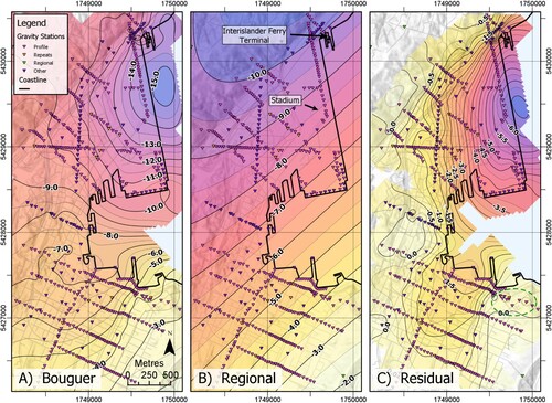
Figure 2. (A) Bouguer gravity anomaly map. Point data gridded using kriging and contoured in mGal. (B) Regional gravity field polynomial. (C) Residual gravity anomaly map. Point data gridded using kriging and contoured in mGal. The green dashed circle denotes an area showing variation in the residual anomaly over bedrock.

where $g_{1980}$ is the gravity calculated from the 1980 international gravity formula for a station’s latitude on the Geodetic Reference System 1980 ellipsoid (Hinze et al. 2005), $g_{fa}$ is the free air correction, $g_{bp}$ is the Bouguer plate correction, $g_{tc}$ is the terrain correction and $g_{bc}$ is the building correction. The free air correction was made assuming a vertical gravity gradient of −0.3086 mGal/m. The Bouguer plate correction was calculated using an assigned crustal density of 2.67 Mg/m³.

Terrain corrections $g_{tc}$ were calculated in Geosoft Oasis Montaj, using DEMs constructed from the 2013 LiDAR-derived 1 m resolution DEM for the Wellington region (LINZ: https://data.linz.govt.nz/) and the 2016 New Zealand Regional Bathymetry 250 m resolution dataset (NIWA: https://niwa.co.nz/our-science/oceans/bathymetry). These were stitched together and resampled to create an inner and an outer DEM, at 2 m resolution (on land) and 10 km radius, and 4 m resolution (on land) and 28 km radius, respectively.

Building correction

Urban areas present additional challenges not usually encountered in gravity surveying, such as the upward pull due to the mass of buildings above the gravity meter ($g_{bc}$). The high precision required for this survey and the close proximity of gravity stations to buildings and infrastructure in urban surveys means this must be corrected for. An approach similar to that used by Dilalos et al. (2018) in Athens, Greece, is used here. A Digital Surface Model (DSM) of buildings and other ground objects was created by calculating the difference between the raw LiDAR data and the LiDAR DEM (which is ground data only). Large stands of trees were then manually clipped out of the resulting DSM, leaving predominately buildings. The DSM data are then treated as ‘terrain’ with an assigned average building density of 0.46 Mg/m³ (Yu 2014). The calculated building corrections were small but non-negligible for this survey, up to 0.2 mGal for stations adjacent to the tallest buildings, with values in the range 0.05–0.10 mGal common in the CBD. In suburban areas away from mid- to high-rise buildings, the building correction was negligible.

Regional residual separation

One of the challenges of interpreted gravity data in plate boundary zones is separating signatures produced by shallow basin and crustal features from deeper crust and mantle sources. The gravity signature of the Wellington region is dominated by the long-wavelength effect of the subducted Pacific plate beneath the lower North Island (Tozer et al. 2017). As Wellington sits 25 km above the plate boundary interface (Henrys et al. 2013) this creates a strong NW-SE gravity gradient across the region (Tozer et al. 2017). In contrast, the sedimentary basin that the Wellington CBD is built on is less than 1 km thick and only ∼1.5 km wide (Kaiser et al. 2019), and thus there should be a clear separation between the long-wavelength regional and short-wavelength residual gravity fields.

We adopt the numerical method used by Stern (1979) to separate the regional and residual fields. A regional gravity field is generated by fitting a two-way, second- or third-order polynomial to the 19 regional stations and 11 of the profiles stations which are on bedrock. The calculated regional field has a SE-NW gradient of ∼2.6 mGal/km across the city (Figure 2(B)). The Root Mean Squared (RMS) error in the fit is 0.4 mGal. The best fit polynomial was selected by plotting a variance of misfit curve against polynomial order, revealing a minimum at the third order (Stronach 2021). Residual gravity anomalies are calculated by subtracting the regional gravity field from the Bouguer anomalies. Notable features in the residual gravity anomaly data (Figure 2(C)) are a strong E-W gradient in Thorndon and Pipitea and an extrapolated maximum amplitude negative anomaly of −6.6 mGal offshore of the Interislander Ferry Terminal.

Two-dimensional modelling

Forward-modelling of the residual gravity anomalies was done on the 15, 2D, profiles using Geosoft Oasis Montaj. Key lithological horizon depths from boreholes near profile lines (Hill et al. 2020) were projected onto the profiles. Stratigraphic interpretations from the GNS Leapfrog model (Kaiser et al. 2019; Hill et al. 2020) were used as a modelling guide where available. Basement rock was assigned a density of 2.67 Mg/m³, and capping sediments assigned lesser densities as detailed below.

DC shifts due to basement weathering

An implicit assumption in the calculation of the regional residual separation is that there is a distinct wavelength separation between deep and shallow gravity effects and that the residuals on basement rock are zero. In this study, negative residuals are observed over some areas of bedrock. In the NW corner of Mount Victoria residual anomalies are −0.5 mGal (green circle in Figure 2(C)), whereas just to the south, residuals on basement rock are +0.2 mGal. We attribute these non-zero residuals to localised variations in the density of greywacke.

Lower density greywacke could occur in distributed fault zones, or in the case of the NW corner of Mount Victoria, in large sea cliffs exposed to weathering. Greywacke’s dry density decreases with weathering; laboratory measurements found a dry density of 2.29 Mg/m³ for ‘moderately weathered’ Wellington greywacke (Brideau et al. 2020). The observed density will be modulated by the level of saturation, particularly in fault zones where rock is fractured and void percentage higher, such as in the suburbs of Mount Victoria or Mount Cook (Figure 1). Therefore, low-density greywacke is likely confined to the hillsides as they are above the water table and undersaturated.

Previous gravity work across the Wellington Fault also calculated non-zero residual anomalies on greywacke hillsides, and Kellett et al. (2017) proposed that the density of greywacke is locally reduced to 2.40–2.50 Mg/m³ to 100 m depth. We also adopt a density of 2.40 Mg/m³ over a similar depth extent for weathered greywacke blocks on each side of the city.

A density of 2.67 Mg/m³ is used in the terrain corrections calculation. For the parts of the city where weathered greywacke is inferred, we model 2.40 Mg/m³ in the weathered greywacke blocks above sea level, which corrects for the higher terrain correction density used in these areas.

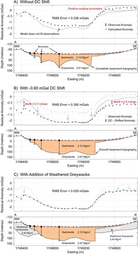
Areas of the low-density basement will locally down warp the regional field, resulting in positive residuals on adjacent areas of basement rock where the density is ‘normal’. Such a warping of the regional field is a numerical consequence of a least squares best fit for a 2D surface. To honour borehole depth constraints for greywacke within the Wellington CBD, we find that the 2D gravity profiles require a small negative adjustment to the residual anomaly, different for each profile, which corrects for the localised warping of the regional field (Figure 3). These adjustments are typically ∼ −0.5 mGal, but range from −0.13 to −1.70 mGal. An adjustment such as this is often referred to as a ‘DC Shift’, a historical term referring to ‘Direct Current’.

Figure 3. The effect of a DC shift and weathered greywacke on model fit. (A) Line A (Figure 1) geological profile with no DC shift, showing the poor fit resulting from honouring the borehole basement constraints. (B) The addition of a −0.8 mGal DC shift, which allows the model to best fit borehole constraints while maintaining smooth, realistic basement topography. This introduces a misfit to the residual anomaly on the hills adjacent to the sedimentary basin. (C) Addition of a zone of weathered greywacke with density 2.4 Mg/m³ on the hills, lowering the calculated anomaly to fit the DC – shifted anomaly.

Sediment density

Kaiser et al. (2019) divide sediments in the Wellington Basin into four units which are also used in this study: anthropogenic fill, shallow sediments, buried sediments, and deeply buried sediments (Table 1). Unit depths in boreholes are the same as those assigned by Kaiser et al. (2019), which was done using a combination of Standard Penetration Test (SPT), shear wave velocity (V_s), lithology, and depth of burial data (2021 email from Matthew Hill, GNS Science). These criteria were used to assign unit depths to some additional boreholes for which this was not already done. Historical records were also used to determine anthropogenic fill depth in some cases.

Table 1. Density data and estimations for each sediment modelling unit.

Unit	Average SPT N-value, (SD)	Average Vs (m/s), (SD)	Empirical density (Mg/m3)	Petlab (Strong et al. 2016) average density (Mg/m3), (# observations, SD)	Semmens (2010) average density (Mg/m3), (# observations, SD)	Hatherton and Sibson (1969) average density (Mg/m3), (# observations, SD)	Assigned density (Mg/m^3)	Average depth to unit base (m)
Anthropogenic Fill	14 (5)	223 (63)	1.86	N/A (0)	2.02 (25, 0.17)	N/A (0)	1.9	4 (where present)
Surface Sediments	29 (5)	287 (30)	1.96	1.96 (11, 0.08)	2.07 (251, 0.14)	2.03 (11, 0.05)	2.0	11
Buried Sediments	58 (23)	432 (39)	2.08	2.13 (17, 0.17)	2.07 (436, 0.16)	2.12 (16, 0.08)	2.1	46
Deeply Buried Sediments	65 (22)	640 (31)	2.2	2.09 (12, 0.15)	N/A (0)	2.36 (3, 0.09)	2.25	159

Notes: SPT N-Values and V_s are averaged between deep boreholes which have data in the database detailed in Hill et al. (2020). Empirical densities were calculated using relationships based on those in Panjamani et al. (2016).

Average densities for these units were estimated using a combination of methods. Direct measurements of sediment density for the Wellington region are available from Petlab (Strong et al. 2016), Semmens (2010), and Hatherton and Sibson (1969), totalling 782 measurements, most of which are from the upper 50 m. Geotechnical data were used to supplement direct density measurements. Generalised empirical relationships between both SPT and density and shear wave velocity and density (Panjamani et al. 2016) have been modified for application to the Wellington region to give density values for the ‘buried sediments’ unit, which is best constrained by direct measurements. The modified equations were then used to estimate downhole densities for ten deep boreholes, and the results averaged with direct measurements (Table 1). The densities assigned to the four units (1.9, 2.0, 2.1, and 2.25 Mg/m³) fall within the range for Quaternary-unconsolidated sediments given by Hatherton and Leopard (1964) (1.75–2.3 Mg/m³) and Tenzer et al. (2011) (2.1 ± 0.2 Mg/m³).

Sources of basin depth uncertainty

The standard error in Bouguer anomalies averages 0.04 mGal, with 95% of errors <0.10 mGal. Four additional sources of uncertainty in the modelled depth to the basement are as follows.

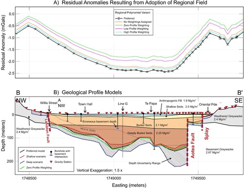
Regional Residual Separation: The choice of the regional polynomial affects the amplitudes of residual anomalies and, therefore, the estimated depth to basement. To analyse the maximum expected difference in basement depth due to the choice of regional field, five different polynomials were created by varying the weighting of each station according to its similarity with adjacent stations. We select the most extreme case polynomial of the five and model to the resultant residual anomaly (green line, Figure 4(A)) on two profile lines, B and J. This test of basin depth sensitivity to the regional residual separation produced basin depths <10% different from those of the preferred model (Figure 4(B)).

Figure 4. Line B residual anomalies and profile model. (A) Residual anomalies resulting from adoption of five different regional fields. The regionals are created by varying the weighting assigned to profile stations as compared to regional stations. The preferred regional (black) derives from a higher weighting to some profile stations and lower to some outlier stations. (B) The geological profile modelled to fit the preferred residual anomaly, with basement contact from the model fitting the ‘zero profile weighting’ regional field (green) and from the shallow and deep interpretations (blue and red) overlain. In each model, only the basement contact is adjusted, while the other layers are kept the same. Note that the depth range of the latter two models entirely encompasses the green line, and this is therefore used to define the depth uncertainty (hashed). The 1969 borehole recording a basement intersection that strongly controls the Hill et al. (2020) model (grey, dashed) and does not fit the gravity model is labelled.

Density: To test the effect of uncertainty in sediment density on modelled basin depths, all sedimentary unit densities on Line A (Figure 1(C)) were increased by 0.1 Mg/m³. This reduced the size of the required DC shift, to −0.5 mGal (from −0.85 mGal) and reduced the thickness of the modelled weathered greywacke by approximately half. Basin depths, however, remained similar as the DC shift adjustment cancels out most of the effect of the increased density.

Two-dimensional approximation: In 2D gravity modelling there is an implicit assumption that geological structure does not vary perpendicular to the profile. Efforts were made to minimise possible 3D effects by designing profile lines perpendicular to basin edges (Figure 1(B)). To quantify possible effects of changes in off-profile basin structure, a 2.5 D modelling approach (Nettleton 1976) was taken on Line H, which is expected to have the most 3D structural variance; 2.5 D modelling allows the introduction of finite strike-lengths of structural bodies into and out of the plane of the interpretation profile. The ‘deeply buried’ sedimentary unit was truncated at 400 m distance from the profile in the SW direction, approximating the decreasing basin depth. This produced a 4% decrease in the calculated gravity anomaly, which then requires a 9% increase in maximum basin depth beneath the profile. Errors due to 3D structural variance on other profiles are expected to be smaller.

Interpretation and DC shift: To assess the effect of DC shifts on basement depth, maximum and minimum basin depth models were constructed for each profile which both fitted borehole depth constraints and was geologically plausible (Figure 4). The DC shift for each line was adjusted, with the RMS error of the fit of calculated to observed gravity allowed to vary by up to 10%. A wider range of possible basin depths is indicated by varying the DC shift than the other model effects, and so the maximum and minimum basin models for each line were used to estimate depth uncertainties.

Results

Fifteen 2D gravity models of the Wellington Basin were produced, the gravity response calculated, and then compared with the observed residual anomalies. An average RMS error of 0.06 mGals was obtained (Table 2). Modelled basement depths in Te Aro agree with the results of previous basin geometry studies (Hill et al. 2020) with the exception of the western end of Line B, near the waterfront (Figure 4). The model of Hill et al. (2020) used greywacke sampled in a borehole drilled near the waterfront in 1969 to constrain basement depth at 61.0 m. The greywacke, however, is not considered to be in situ as modelled gravity anomalies indicate that the basement is ∼144 m deep at this location, and no plausible gravity model will fit the shallower, 61 m depth for basement at the borehole site. All depths reported here are in metres below ground level, in order that values also give sediment thickness and thus an indication of earthquake shaking amplification. Depths in metres below sea level are given in the supplementary data.

Table 2. Key parameters for each profile. Max constrained basement depth is the maximum depth directly beneath a gravity station.

Profile parameters
Line	Length (m)	# Stations	Max Anom. (mGal)	DC shift (mGal)	RMS error (mGal)	Max constrained basement depth (m)
A	1680	42	−1.35	0.85	0.03	130
B	2260	53	−1.74	0.70	0.10	155
C	1620	41	−1.21	0.60	0.02	100
D	1030	34	−0.57	0.13	0.03	30
G	1530	32	−1.89	1.30	0.06	150
H	1530	28	−3.85	0.65	0.11	270
I	1710	31	−5.05	0.64	0.08	430
J	1970	43	−6.18	0.46	0.05	470
K	1120	16	−5.85	0.30	0.03	460
N	280	7	−3.60	1.10	0.11	150
P	790	9	−5.32	1.65	0.08	400
Q	1580	–	−6.26	1.70	0.05	–
T	1110	26	−2.62	0.45	0.05	130
U	1600	34	−5.48	0.70	0.03	430
W	360	17	−1.74	0.62	0.05	150

Note: Line Q was constructed using interpolated residual anomaly values rather than data measurements, and therefore does not have a maximum ‘constrained’ depth.

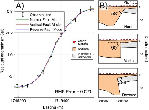
All five lines which cross the Aotea Fault show vertical basement offsets, with a maximum of 130 m on Line B (Figure 4(B)). A better fit to the residual gravity anomaly is obtained if the basement offset occurs in two steps, of 30 and 100 m, separated by 100 m horizontally and with the latter step aligning with the inferred location of the Aotea Fault (Hill et al. 2020). The interpretation of two basement offset steps is consistent with residual anomalies on Line A, but not on Lines C and D, so the splay is interpreted to either re-join the main fault (Figure 7) or terminate north of Line C. Without constraint on the location of the surface trace of the Aotea Fault onshore in Wellington, the dip of the main fault was not able to be determined from gravity data, with a range from 58° normal, to 80° reverse fitting the residual anomalies equally well (Figure 5). However, in Wellington Harbour, the Aotea Fault has been interpreted to be a steeply dipping reverse fault based on multichannel seismic data (Barnes et al. 2019).

Figure 5. Dip sensitivity testing on Line A. (A) Observed residual anomalies with calculated gravity for each of the three models on right. (B) Fault models show the maximum possible normal and reverse dips for the Aotea Fault which do not increase the RMS error of the fit to observations of 0.029 mGal.

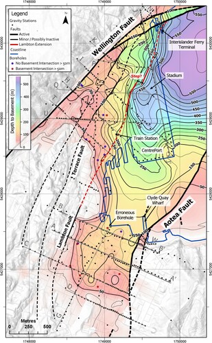
Few borehole constraints on basement depth are available in Thorndon and Pipitea, and here depths modelled in this study diverge from previous studies (Semmens 2010; Kaiser et al. 2019; Hill et al. 2020). In Thorndon, depths are ∼50 m shallower, and in Pipitea 200–300 m deeper than modelled by Kaiser et al. (2019). Near the Wellington Stadium, basement depths reach an onshore maximum of 540 m on Line P, 330 m deeper than Kaiser et al. (2019). Gravity models indicate a deep subbasin that extends from Pipitea into Te Aro and likely extends offshore past the Interislander Ferry Terminal, where basement depths of >600 m are inferred (Figure 7). A steep gradient in the gravity anomaly beneath Wellington Stadium is consistent with a basement dip of >40° to the east (Figure 2(C)). We interpret the steep step down in the basement here to be produced by movement on a northern extension of the Lambton Fault (Grant-Taylor 1963). Other steep basement offsets modelled on gravity profiles on the western side of Wellington City may be attributed to offsets on the Terrace Fault and a still-unnamed fault. (Figure 7) (Grant-Taylor 1963; Grant-Taylor et al. 1974).

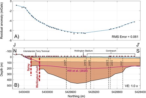
On Lines J and N, in the vicinity of the Interislander Ferry Terminal (Figures 1 and 7) the Wellington Fault is modelled as a main fault with a secondary splay (Figure 6). In the absence of other information, this would have been modelled as a single fault at the location labelled ‘splay’. However, Perrin (1993) locates the Wellington Fault with confidence at its position in Figure 6, on the basis of borehole sediment correlation. In order to honour both the interpretation of Perrin (1993) and the residual gravity anomaly, two fault offsets are modelled.

Figure 6. Profile for Line J. (A) Observed residual anomalies and calculated gravity response due to the geological model. (B) Geological model with basement contact from Hill et al. (2020) for this profile in purple. Gravity stations are red triangles, and intersections with other profile lines are marked in black. There are no deep boreholes on this profile.

3D basement depth map

3D gravity modelling would usually use an iterative inversion process (Li and Oldenburg 1998). Geosoft Oasis Montaj does not allow for variations in DC shift in a 3D inversion as are required here, and so our method of constructing a 3D contour map of basement depth is to combine a series of 2D gravity profiles.

Point data from the best fitting, maximum and minimum basement depth models were gridded at 10 m resolution using a spline function. Wellington, Aotea, and additional secondary minor faults traces were used as barriers to the spline function, thus introducing vertical structural offsets into the model. Basement depth constraints from all boreholes were also included to constrain the spline function. The spline function was subtracted from the DEM to generate a map of basement depth from the surface (Figure 7). This basement depth map was checked against deep boreholes that did not intersect basement to test its validity.

Figure 7. Preferred basin depth map produced by kriging point data extracted from profile models and contoured in metres. Profile lines labelled in grey. Fault traces located with moderate to high confidence from seismic, gravity or geologic data are solid black lines, inferred fault traces dashed black lines. The proposed extension to the Lambton Fault is in red.

Maximum and minimum basin depth models

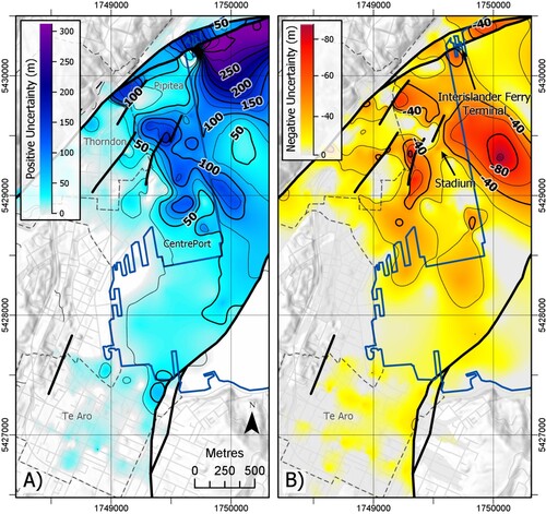
The difference between the preferred model and the minimum depth model is an estimation of the uncertainty in the negative (i.e. shallower basement) direction (Figure 8(A)), while the difference between the preferred model and the maximum depth model is an estimation of uncertainty in the positive (i.e. deeper basin) direction (Figure 8(B)). Negative depth uncertainties are small, mostly ∼20 m or less. This is a key result, as it indicates that the large basement depths modelled in Pipitea are real and are significantly deeper than previous estimates. Positive basement depth uncertainties are larger, increasing from west to east across Thorndon and Pipitea, with an onshore maximum depth uncertainty of >150 m near the deepest onshore area, beneath the Wellington Stadium. Based on the uncertainty map, the greatest onshore basement depth may be as much as 640 m. In Wellington Harbour near the Interislander Ferry Terminal, the maximum positive depth uncertainty is ∼300 m, but this is poorly constrained.

Figure 8. (A) Map of the difference between the preferred depth map and the deep interpretation, representing depth uncertainty in the positive, that is, deeper direction. (B) Map of the difference between the preferred depth map and the shallow interpretation, representing depth uncertainty in the negative, that is, shallower direction.

Discussion

This study’s most important results are three-fold: the basement depths found in Pipitea and likely offshore that are significantly (∼300 m) greater than those proposed by previous studies; the proposed extension to the Lambton Fault, running roughly from Wellington Railway station due north to the Interislander Ferry terminal (Figure 7); and the onshore expression of the Aotea fault.

Previous studies (Kaiser et al. 2019; Hill et al. 2020) use fundamental site period measurements to model basin depths in the Pipitea/CentrePort area where deep boreholes are not available but note that 3D amplification effects would affect the reliability of these estimates. Based on our model, 3D effects would be expected as seismic energy reflects from the steep faults modelled in Thorndon (Figure 7) as well as from the Wellington Fault. Kaiser et al. (2019) also note that an impedance contrast within the sediments could lead to an erroneously shallow estimate for bedrock. These reasons could explain the apparent underestimation of bedrock depth.

The lesser sedimentary thicknesses adopted in the previous earthquake shaking studies (Benites and Olsen 2005) in the Pipitea and CentrePort area indicate that the hazard potential of this part of Wellington may have been underestimated. For example, 3D simulations of earthquake amplification for the Wellington – Hutt Valley region predict the strongest horizontal ground motion in the Wellington Harbour area, where the sediment thickness is proposed to be ∼600 m (Benites and Olsen 2005). In the Pipitea – CentrePort region (Figure 1), where they adopt ∼200 m for the sediment thickness (Benites and Olsen 2005), shaking is proposed to be much less. Our new model, however, suggests ∼450 m of sediment in this part of the CBD, and hence the region of maximum shaking is also likely to extend into this vulnerable part of the city.

Our models indicate the Lambton Fault delineates the edge of a subbasin that dips steeply to the east rather than a shallow and broad dip to the northeast as indicated by previous models (Kaiser et al. 2019). In detail, the depth contours suggest a right step (facing north) (Figure 7), which if the Lambton Fault sense of movement is dextral, the same as the Wellington Fault, would mean the area to the south of the step is under tension, resulting in enhanced subsidence. This could explain the >450 m basement depths in this area, although structures of this size are near the resolution limit of a gravity survey. Definition of the apparent complex structure in this area will be essential for future earthquake shaking models, which might be done with more gravity data or targeted seismic surveys.

On a larger scale, the Wellington Fault also bends, or steps, to the right as it passes to the north from the CBD, which again implies an element of extensional deformation during earthquakes. The maximum depths seen in the study area, offshore of the Interislander Ferry Terminal, would be a result of this deformation and will be another important target area to define with future work, given the proximity to rail and shipping infrastructure.

Results of this study concur with that of Barnes et al. (2019) on the Aotea Fault, who identify a steep reverse dip and the fault tracking onshore at the northern end of Clyde Quay Wharf (Figure 7). While the dip of the Aotea Fault could not be constrained from the gravity data, the reverse model presented (Figure 5) fits the data and concurs with the Barnes et al. interpretation. With a vertical basement offset of up to 130 m, the Aotea Fault along with the Wellington Fault gives the Wellington Basin two sharp, near vertical and parallel margins, which would be likely to reflect seismic energy between them and cause reverberation and resonance effects during an earthquake.

Conclusions

We undertook a high precision gravity survey across the Wellington CBD, the first such survey since 1969. Key findings are:

• Residual anomalies across the city are on the order of a few mGal, with the largest amplitude anomaly of −6.2 mGal near the Wellington Stadium in Pipitea. Uncertainties are at most ±0.1 mGal, with an average of ±0.04 mGal.

• The maximum thickness of the sediments in the Wellington CBD modelled in this study is 540 +100/−50 m in the Pipitea – CentrePort area. Maximum amplification of earthquake shaking in the Wellington region is likely to occur here and in parts of the harbour just to the north.

• Gravity data outline the onshore extension of the Aotea fault to pass south along the western margin of Mt Victoria, with a vertical basement offset of up to 130 m, suggesting a strong component of vertical motion.

• A northward extension to the Lambton Fault is proposed, manifested as a steep, east-dipping basement surface beneath the Wellington Train Station and railway yards. Basement depth contours suggest fault stepping, resulting in a small pull-apart sub-basin beneath part of the Pipitea – CentrePort region of Wellington City.

Acknowledgements

The authors thank all staff and students at Victoria University of Wellington who contributed to this project, as well as staff at GNS Science who assisted with technical matters and site access. The authors thank Dr W. Stratford (GNS) for reviewing the manuscript. The authors thank Dr A. Pancha (Aurecon NZ Ltd) for data sharing and assistance and staff at CentrePort Ltd for facilitating site access.

Disclosure statement

No potential conflict of interest was reported by the author(s).

Data availability statement

The authors confirm that the data supporting the findings of this study are openly available in Mendeley Data at http://doi.org/10.17632/j2txy867b4.1. The data are also planned to be available from the GNS Science gravity database, accessible through the E Tūhura – Explore Zealandia portal: https://data.gns.cri.nz/tez/. Further details of methods used in this study are available from the Victoria University of Wellington library: https://doi.org/10.26686/wgtn.15176061.v1 (Stronach 2021).

Additional information

Funding

Funding for this project was provided by New Zealand Earthquake Commission Biennial Grant #20795, the New Zealand Society of Earthquake Engineering, Geoscience Society of New Zealand, QuakeCoRE and Wellington Branch of the Royal Society. The authors thank them for their support.

References

- Barnes PM, Nodder SD, Woelz S, Orpin AR. 2019. The structure and seismic potential of the Aotea and Evans Bay faults, Wellington, New Zealand. New Zealand Journal of Geology and Geophysics. 62(1):46–71.
- Begg JG, Mazengarb C. 1996. Geology of the Wellington area. Lower Hutt: GNS Science.
- Benites R, Olsen K. 2005. Modeling strong ground motion in the Wellington metropolitan area, New Zealand. Bulletin of the Seismological Society of America. 95(6):2180–2196.
- Bradley B, Wotherspoon L, Kaiser A. 2017. Ground motion and site effect observations in the Wellington region from the 2016 Mw7.8 Kaikōura, New Zealand earthquake. Bulletin of the New Zealand Society for Earthquake Engineering. 50:94–105.
- Bradley B, Wotherspoon L, Kaiser A, Cox B, Jeong S. 2018. Influence of site effects on observed ground motions in the Wellington region from the Mw 7.8 Kaikoura, New Zealand. Earthquake: Bulletin of the Seismological Society of America. 108:1722–1735.
- Brideau Marc-André, Massey Christopher I, Carey Jonathan M., Lyndsell Barbara. 2020. Geomechanical characterisation of discontinuous greywacke from the Wellington region based on laboratory testing. New Zealand Journal of Geology and Geophysics:1–18.
- Cowan M, Hatherton T. 1968. Gravity surveys in Wellington and Hutt Valley. New Zealand Journal of Geology and Geophysics, 11(1):3–15.
- Dilalos S, Alexopoulos J, Tsatsaris A. 2018. Calculation of building correction for urban gravity surveys: a case study of Athens metropolis (Greece). Journal of Applied Geophysics, 159:540–552.
- Edbrooke SW, Heron DW, Forsyth PJ, Jongens R. 2017. The Geological Map of New Zealand. Lower Hutt, New Zealand: GNS Science.
- Francois-Holden C, Kaiser A. 2013. Sources, ground motion and structural response characteristics in Wellington of the 2013 Cook Strait earthquakes. Bulletin of the New Zealand Society for Earthquake Engineering. 46:188–195.
- Grant-Taylor TL. 1963. Geological faults in the Wellington area. New Zealand Institute of Architects Journal, 30(4):68–69.
- Grant-Taylor TL, Adams RD, Hatherton T, Milne JDG, Northey RD, Stephenson WR. 1974. Microzoning for earthquake effects in Wellington, N.Z. DSIR bulletin no. 213. Lower Hutt, New Zealand: Department of Scientific and Industrial Research.
- Grapes R, Downes G. 1997. The 1855 Wairarapa, New Zealand, earthquake – analysis of historical data. Bulletin of the New Zealand Society for Earthquake Engineering, 30(4), 271–368.
- Grose DT, Knappstein MA, Peters NC, Symmans BS. 2015. 12th Australia - New Zealand Conference on Geomechanics. Wellington.
- Hamling I, Hreinsdottir S, Clark K, Elliott J, Liang C, Fielding E, Litchfield N, Villamor P, Wallace L, Wright T, et al. 2017. Complex multifault rupture during the 2016 M w 7.8 Kaikōura earthquake, New Zealand. Science, 356:eaam7194.
- Hammer S. 1939. Terrain corrections for gravimeter stations. Geophysics, 4(3):189–194.
- Hatherton T, Leopard AE. 1964. The densities of New Zealand rocks. New Zealand Journal of Geology and Geophysics. 7(3):605–625.
- Hatherton T, Sibson RH. 1969. A gravity survey of Wellington city. Lower Hutt, New Zealand: Department of Scientific and Industrial Research.
- Henrys S, Wech A, Sutherland R, Stern T, Savage M, Sato H, Mochizuki K, Iwasaki T, Okaya D, Seward A, et al. 2013. SAHKE geophysical transect reveals crustal and subduction zone structure at the southern Hikurangi margin, New Zealand. Geochemistry, Geophysics, Geosystems. 14:2063–2083.
- Hill MP, Kaiser AE, Bourguignon S, Bruce ZR. 2020. Wellington City Council seismic microzonation map – adoption of NZS1170.5 Subsoil classifications. Lower Hutt, New Zealand: GNS Science.
- Hinze W. 2003. Bouguer reduction density, why 2.67? Geophysics. 68(5):1559–1560.
- Hinze W, Aiken C, Brozena J, Coakley B, Dater D, Flanagan G, Forsberg R, Hildenbrand T, Keller R, Kellogg J, et al. 2005. New standards for reducing gravity data: The North American gravity database. Geophysics. 70:J25–J32.
- Kaiser A, Bourguignon S, Hill M, Wotherspoon L, Bruce Z, Morgenstern R, Giallini S. 2019. Updated 3D basin model and the NZS 1170.5 subsoil class and site periods maps for the Wellington CBD. Project 2017-GNS-03-NHRP: GNS Science Consultancy Report, v. 2019/01, p. 48.
- Kearey P, Brooks M, Hill I. 2002. An introduction to geophysical exploration, 3rd edition, 272 p. Oxford: Blackwell Publishing.
- Kellett RL, Black JA, Brune R, Stagpoole VM, O’Brien G. 2017. Gravity survey of the Hutt valley: modelling the wellington fault. GNS Science Consultancy Report, v. 2017/24, p. 23.
- Langridge R, Van Dissen R, Rhoades D, Villamor P, Little T, Litchfield N, Clark K, Clark D. 2011. Five thousand years of surface ruptures on the Wellington fault, New Zealand: implications for recurrence and fault segmentation. Bulletin of The Seismological Society of America. 101:2088–2107.
- Li Y, Oldenburg DW. 1998. 3-D inversion of gravity data. Geophysics. 63(1):109–119.
- Little TA, Van Dissen R, Schermer E, Carne R. 2009. Late Holocene surface ruptures on the southern Wairarapa fault, New Zealand: link between earthquakes and the uplifting of beach ridges on a rocky coast. Lithosphere. 1:4–28.
- McNally KC, González-Ruiz JR, Stolte C. 1986. Seismogenesis of the 1985 great (Ms=8.1) Michoacan, Mexico earthquake. Geophysical Research Letters. 13(6):585–588.
- Mouslopoulou V, Nicol A, Little TA, Walsh JJ. 2007. Terminations of large strike-slip faults: an alternative model from New Zealand. Geological Society, London, Special Publications. 290:387–415.
- Nettleton LL. 1976. Gravity and magnetics in oil prospecting. New York. McCraw-Hill.
- Panjamani A, Uday A, Moustafa S, Alarifi N. 2016. Correlation of densities with shear wave velocities and SPTN values. Journal of Geophysics and Engineering. 13:320–341.
- Perrin ND. 1993. Location of Wellington fault in relation to Thorndon overbridge, Wellington urban motorway. Lower Hutt, New Zealand: Institute of Geological and Nuclear Sciences.
- Rhoades D, Van Dissen R, Langridge R, Little T, Ninis D, Smith E, Robinson R. 2011. Re-evaluation of conditional probability of rupture of the Wellington-Hutt Valley segment of the Wellington fault. Bulletin of the New Zealand Society for Earthquake Engineering. 44, 77–86.
- Robertson EI, Reilly WI. 1960. The New Zealand primary gravity network. New Zealand Journal of Geology and Geophysics. 3(1):41–68.
- Semmens S. 2010. An Engineering Geological investigation of the seismic Subsoil classes in the Central Wellington commercial area [MSc]. Christchurch, New Zealand: University of Canterbury.
- Septentrio NV. 2017. Septentrio Altus NR3 User Manual. Leuven, Belgium.
- Stagpoole V. 2018. Description of the data in the GNS gravity database. Lower Hutt, New Zealand: GNS Science.
- Stagpoole V, Tontini FC, Fukuda Y, Woodward D. 2021. New Zealand gravity reference stations 2020: history and development of the gravity network. New Zealand Journal of Geology and Geophysics. 0:1–12.
- Standards New Zealand. 2004. Structural design actions – part 5: earthquake actions – New Zealand (NZS 1170.5:2004). Wellington: Standards New Zealand.
- Stern TA. 1979. Regional and residual gravity fields, central North Island, New Zealand. New Zealand Journal of Geology and Geophysics. 22(4):479–485.
- Stronach AI. 2021. Basin depth mapping beneath Wellington city based on residual gravity anomalies [MSc]. Wellington, New Zealand: Victoria University of Wellington.
- Strong DT, Turnbull RE, Haubrock S, Mortimer N. 2016. Petlab: New Zealand’s national rock catalogue and geoanalytical database. New Zealand Journal of Geology and Geophysics. 59(3):475–481.
- Styles P, Toon S, Thomas E, Skittrall M. 2006. Microgravity as a tool for the detection, characterization and prediction of geohazard posed by abandoned mining cavities. First Break. 24(5):51–60.
- Tenzer R, Sirguey P, Rattenbury M, Nicolson J. 2011. A digital rock density map of New Zealand. Computers & Geosciences. 37(8):1181–1191.
- Tozer B, Stern TA, Lamb SL, Henrys SA. 2017. Crust and upper-mantle structure of Wanganui Basin and southern Hikurangi margin, North Island, New Zealand as revealed by active source seismic data. Geophysical Journal International. 211(2):718–740.
- Vantassel J, Cox B, Wotherspoon L, Stolte A. 2018. Mapping depth to bedrock, shear stiffness, and fundamental site period at CentrePort, Wellington, using surface-wave methods: Implications for local seismic site amplification. Bulletin of the Seismological Society of America. 108, 1709–1721.
- Walcott RI. 1987. Geodetic strain and the deformational history of the North Island of New Zealand during the late Cainozoic. Philosophical Transactions of the Royal Society of London. Series A, Mathematical and Physical Sciences. 321:163–181.
- Yu D. 2014. The influence of buildings on urban gravity surveys. Journal of Environmental and Engineering Geophysics. 19(3):157–164.
- Yule DE, Sharp MK, Butler DK. 1998. Microgravity investigations of foundation conditions. Geophysics. 63(1):95–103.