Stressor-response relationships and the prospective management of aquatic ecosystems

ABSTRACT

Scientists and environmental managers use stressor-response (S-R) relationships to characterise and predict ecological and socioeconomic responses to anthropogenic stressors in lakes and other aquatic ecosystems. S-R relationships with thresholds (stressor levels beyond which small increases cause large responses) are reported with increasing frequency. Threshold responses pose risks of unanticipated degradation, but also provide a stimulus for shifting environmental management strategies from retrospective (focused on post-hoc responses to degradation) to prospective (focused on preventing degradation). We set out a framework for interpreting S-R relationships in terms of functional forms, trajectories, thresholds and slopes. These characteristics convey information about resistance to degradation and recovery, risks of threshold exceedance, and alternate stable states. We then set out steps for implementing threshold-based management strategies, which are based on forecasting S-R relationships and carrying out preventative actions within an adaptive framework. Prospective, threshold-based management is a challenging yet promising alternative to the prevailing retrospective strategies.

KEYWORDS:

• Stressor-response relationships
• ecological thresholds
• resistance
• sensitivity
• forecasting
• prospective environmental management
• aquatic ecosystems

Introduction

Stressor-response (S-R) relationships are widely used in environmental science to characterise and predict effects of contaminant loading, water abstraction, acidification, warming and other anthropogenic stressors on aquatic ecosystems (Adams 2003; Abell et al. 2012; Nichols et al. 2017; Rosenfeld 2017). S-R relationships are used most frequently to characterise and predict ecological degradation as stressor levels increase, but they can also be used to characterise and predict recovery as stressor levels decline (Kemp et al. 2009; Zhao et al. 2013).

S-R relationships are used in environmental management as well as science; management applications include regulating contaminant discharges, evaluating restoration projects, and predicting effects of changes in stressor levels in unmonitored locations and in the future (e.g. Clements et al. 2010; Flynn et al. 2015; Mouquet et al. 2015). Forecasting the trajectories of S-R relationships to guide management decisions is at an early stage of development, but is growing rapidly (Pace et al. 2015; Petchey et al. 2015; Dietze et al. 2018). For example, regulatory agencies are using nutrient load-hypoxia relationships to forecast lake and coastal hypoxia in response to future changes in nutrient input from land, and to set nutrient load targets that will prevent hypoxia from occurring (Scavia et al. 2016; Testa et al. 2017).

This paper presents a rationale for using S-R relationships as a basis for prospective, threshold-based management of aquatic ecosystems. Many of the examples cited come from lake research and management, but the framework is applicable to all aquatic ecosystems at risk from future increases in stressor levels. Threshold-based management refers to management strategies that are predicated on the ability to forecast pending thresholds in S-R relationships and on management actions that prevent threshold crossing. Threshold-based management is a subset of a larger class of prospective strategies that rely on ecological forecasting (Hobbs RJ et al. 2011; Kelly et al. 2014, 2015; Lewison et al. 2015).

In the second section, we set out a framework for characterising S-R relationships in terms of direction (degradation, recovery), functional form (e.g. logistic, exponential), and other properties of bivariate relationships (e.g. thresholds, slopes, intercepts). We define thresholds broadly as changes in the slopes of S-R relationships beyond which small increases in stressor levels cause large responses (Groffman et al. 2006). These characteristics of S-R relationships are basic elements of ecological forecasting (Dietze 2017). The S-R relationships discussed in this paper are associated with near-term (daily to decadal) forecasts, which we distinguish from multi-decadal forecasts of responses to climate change (Petchey et al. 2015; Dietze et al. 2018). We focus on monotonic, bivariate relationships and exclude multiple-stressor situations due to current limits to forecasting proficiency (Darling and Côté 2008; Harley et al. 2017). Improved understanding of bivariate S-R relationships is a prerequisite for understanding multiple stressor situations (Halpern and Fujita 2013). The additional information needed to incorporate multiple-stressor-response relationships in prospective management strategies are discussed in the fourth section.

In the third section, we discuss the basic steps needed to implement threshold-based management strategies. These strategies are widely discussed but rarely implemented, due in part to uncertainties in forecasting (Oliver and Roy 2015; Dietze et al. 2018). Our discussion covers selecting, characterising and forecasting S-R relationships, developing management triggers, and using adaptive management frameworks to improve the chances that management actions will prevent threshold crossing and subsequent degradation.

In the fourth section, we make a case for widespread implementation of prospective management of aquatic ecosystems, based on recent improvements in ecological forecasting. Although forecasts can never be entirely certain, we contend that prospective management actions based on informed albeit uncertain forecasts are likely to have better outcomes than retrospective management (actions taken after degradation has occurred) or inaction.

Characteristics of S-R relationships

The simplest S-R relationships are linear, where a unit change in the stressor elicits a proportional response over the entire stressor range. Linear S-R relationships are appealing in terms of interpolation and forecasting, but nonlinear S-R relationships with thresholds are being reported with increasing frequency, and it has been suggested that S-R relationships in natural ecosystems are predominantly nonlinear (e.g. Bestelmeyer et al. 2011; Selkoe et al. 2015). However, recent reassessments of nonlinear S-R relationships reported from aquatic ecosystems indicated that the evidence presented for threshold behaviour is generally weak (MacNally et al. 2014; Capon et al. 2015). Thus, the actual prevalence of linear versus nonlinear S-R relationships remains an open question.

In this paper, we focus on nonlinear S-R relationships for three reasons. First, S-R relationships that appear linear based on existing data may prove to be nonlinear when their stressor data ranges are extended, as discussed below. Second, while forecasting nonlinear responses is more challenging than forecasting linear responses, it is essential to consider nonlinear responses due to the risk of disproportionate degradation if stressor levels exceed thresholds. Third, there is an attendant risk that severely degraded ecosystems will fail to recover when stressor levels are subsequently reduced. These risks provide the rationale for the emerging field of threshold-based management (Kelly et al. 2014; Liu et al. 2015; Selkoe et al. 2015).

Stressor and response variables

Some S-R relationships represent direct, causal links between stressors and responses, e.g. between toxicant exposure and mortality (Wu et al. 2012). In other cases, S-R relationships are based on correlative associations where the effects of the stressor variables are understood to be indirect, as in correlations between catchment impervious surface area and lake water quality (Coats et al. 2008). Other catchment variables used as proxies for direct stressors include agricultural and urban land cover and human population densities (Gergel et al. 2002; Abell et al. 2011). Catchment-scale proxy variables often leave substantial unexplained variation in in S-R relationships, but they are widely used due to the availability of data and because they are closely linked to land-management actions (Gergel et al. 2002; Abell et al. 2011; Feld et al. 2016).

The response variables in S-R relationships correspond to either valued environmental attributes that decrease with increasing anthropogenic stress (e.g. biodiversity, rare species populations), or to symptoms of degradation that increase with increasing stress (e.g. algal biomass). The selection of stressor and response variables used to derive S-R relationships is discussed in detail in the third section.

Functional forms and characteristics of S-R relationships

Whether they represent causal or correlative relationships, S-R relationships can be described using mathematical functions and their characteristics (e.g. intercepts, thresholds, slopes, inflection points). The most widely recognised S-R relationships correspond to four general functional forms: linear, logistic, logarithmic, and exponential (Figure 1A–D). These functions can apply to both degradation trajectories (from low to high stressor levels) and recovery trajectories (from high to low stressor levels). The functions that correspond to different S-R relationships may be selected based on theoretical models of those relationships (e.g. saturable growth in nutrient-limited phytoplankton, exponential declines in populations of contaminant-sensitive species). Observational data can then be fitted to the selected model and the goodness of fit tested (Filstrup et al. 2014).

Figure 1. Typology of theoretical S-R relationships. Arrows indicate stressor thresholds. A, Linear relationship with constant sensitivity over the stressor range. B, Logarithmic relationship with relatively high sensitivity at low stressor levels and high resistance at high stressor levels. C, Exponential relationship with high resistance at low stressor levels and high sensitivity at high stressor levels. D, Logistic relationship with high resistance at high and low stressor levels, and high sensitivity near the inflection point. E, Logistic relationship with degradation and recovery trajectories offset by an interval of the stressor range. F, Logistic relationship with bifurcation. The response variable can occupy two or more different states at stressor levels that fall within the bifurcation range, indicated by the dotted arrows. Within the range of bifurcation, the responses to changes in stressor levels are unstable and can oscillate. At stressor levels increasingly divergent from the range of bifurcation, the system stabilises in one state.

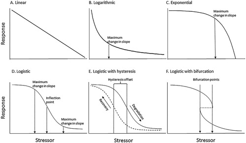
By definition, nonlinear S-R relationships include domains of resistance to stress (i.e. stressor ranges over which there is relative little response), and domains of sensitivity (stressor ranges over which there are relatively large responses). Domains of resistance are indicated by near-horizontal segments on plots of S-R relationships, and domains of sensitivity are indicated by steeply sloping segments. For S-R relationships that correspond to negative logarithmic and negative exponential functions (Figure 1B,C), the primary domains of resistance are at high and low stressor levels, respectively. For S-R relationships that correspond to logistic functions there are domains of resistance at both high and low stressor ranges, separated by a domain of high sensitivity (Figure 1D). Resistance applies to both increases in stressor levels (i.e. resistance to degradation) and reductions in stressor levels (i.e. resistance to recovery). Among the most familiar cases of high resistance to recovery are lakes that are degraded by anthropogenic eutrophication, then fail to recover in response to reductions in nutrient loading (Bennion et al. 2015).

Resistance, recovery and hysteresis

The term resistance as used in this paper refers to the capacity of an ecological property (i.e. a response variable) to resist changes in state when exposed to varying stressor levels. This usage contrasts with ‘ecological resilience’, which refers to the degree of recovery in a given time period following perturbations (Holling 1996; Hodgsen et al. 2015). We note that resistance can be evaluated directly from S-R relationships whereas resilience cannot, because it is defined by a temporal dimension.

The mechanisms that confer resistance to stressors are termed stabilising (or negative) feedbacks (Holling 1973; Nyström et al. 2012). In contrast, destabilising (or positive) feedbacks are mechanisms that increase sensitivity to a stressor. Stabilising and destabilising feedback can affect both degradation and recovery trajectories of S-R relationships. Stabilising feedback mechanisms that inhibit degradation include a wide range of compensatory processes, such as increased herbivory in response to algal proliferations and increased denitrification in response to increased nitrate input (e.g. Ghedini and Connell 2016) (Table 1). Functional redundancy (i.e. the presence of multiple taxa with similar ecological roles) can increase the effectiveness of those compensatory processes and ensure that they continue if sensitive taxa are lost (Frost et al. 1995). Stabilising feedback mechanisms that inhibit recovery from degradation, despite reductions in stressor levels, include competitive exclusion of foundational species such as lake macrophytes (by phytoplankton) corals (by macroalgae and sponges) (Nyström et al. 2012). Destabilising feedback mechanisms that accelerate or worsen degradation include biogeochemical changes (e.g. sediment anoxia) that increase nutrient loading (Folke et al. 2004) and reductions in algae consumers due to habitat degradation or fishing pressure, which contributes to algal proliferations (Hughes et al. 1987, 2017).

Table 1. Examples of naturally occurring biological, hydrological and chemical feedback mechanisms in lake ecosystems that confer resistance to degradation, and interventions that enhance the effects of those mechanisms.

Natural feedback mechanisms	Interventions that enhance resistance
1. Sediment stabilisation and suppression of sediment resuspension by macrophytes.	Macrophyte enhancement by water level management (Van Geest et al. 2007), propagule sowing (Rowe and Champion 1994), and planting (Hilt et al. 2006).
2. Removal of dissolved nutrients from enriched lake water by littoral and floating plants.	Artificial floating islands composed of buoyant platforms and plants assimilate dissolved nutrients; plant biomass periodically removed (Yeh et al. 2015).
3. Suppression of phytoplankton proliferations by zooplankton, bivalves and other phytoplankton grazers.	Foodweb biomanipulation to enhance grazing pressure (Reynolds 1994; Burns et al. 2014).
4. Removal of nitrate by bacterial denitrification and anammox.	Enhanced denitrification and anammox through engineered structures that increase interstitial flow and organic matter amendments (Pierce et al. 2012; Merill and Tonjes 2014).
5. Flushing and dilution of turbid or nutrient-rich lake water with tributary or oceanic water.	Managed lake openings (Schallenberg et al. 2010), augmented inflows (Welch 1981; Lundgren et al. 2013), and siphoning (Hickey and Gibbs (2009) to increase flushing and dilution rates.
6. Suppression of cyanobacterial blooms by turbulent mixing and temperature reduction.	Artificial mixing and destratification by aeration and pumping systems (Bormans et al. 2016; Visser et al. 2016).
7. Phosphorus sequestration by metal-binding in lake bed sediments.	Application of aluminium-based P capping agents (Hickey and Gibbs 2009)
8. Suppression of phosphorus desorption by hypolimnetic oxygen	Whole-lake aeration or hypolimnetic oxygenation without mixing (Hickey and Gibbs 2009)

Note: Potential applications of the interventions in shallow and deep lakes are shown in Figure 2.

In cases where there is minimal resistance to recovery, decreasing stressor levels can result in recovery along a trajectory that mirrors the degradation trajectory; these cases correspond to the ‘rubber band model’ proposed by Saar (2002) and Lake et al. (2007). In cases where stabilising feedback inhibits recovery, degradation and recovery follow dissimilar trajectories; these cases correspond to the ‘hysteresis model’ (Scheffer et al. 2001; Saar 2002; Elliott et al. 2007 Lake et al. 2007). Although the terms hysteresis and recovery time lags are occasionally conflated, we follow the definition used in the references listed above for the hysteresis model, which refers to differences in degradation and recover trajectories in response the changing stressor levels, not to temporal variation. In some cases of hysteresis, degradation and recovery trajectories are similar in shape, but are offset by some interval along the stressor axis. Offset hysteresis occurs most frequently when degradation and recovery trajectories primarily differ in their domains of resistance (Figure 1E). In other cases, degradation and recovery trajectories differ substantially over a broad stressor range (Jeppesen et al. 2005; Bennion et al. 2015. Furthermore, recovery trajectories do not always return a response variable to a given reference state or baseline when the corresponding stressor is reduced to its own reference state or baseline. Failure to fully recovery may be caused by historical shifts in baselines caused by factors other than the stressor of concern (e.g. climate warming), and to resistance associated with stabilising feedback (Kopf et al. 2015). These cases have been termed ‘irreversible’ (Carpenter et al. 1999; Davis et al. 2010), but that conclusion may not be warranted if recovery can be achieved through interventions other than direct stressor reduction such as biomanipulation (e.g. Anttila et al. 2013).

In some cases of hysteresis, the trajectory of the S-R relationship bifurcates at a threshold (the ‘bifurcation point’), beyond which two dissimilar trajectories can occur over the same stressor range and the response variable occupies one of two alternative states (Figure 1F). Bifurcation can occur on both degradation and recovery trajectories (Scheffer et al. 2001). When strong stabilising feedback inhibits further change in both states, they are referred to as ‘alternative stable states’ (Beisner et al. 2003; Schröder et al. 2005). The most widely recognised cases of alternative stable states are those where ‘healthy’ and ‘degraded’ ecosystem states both occur over the same stressor range. Examples of paired healthy and degraded systems include clear, macrophyte-dominated and turbid, phytoplankton-dominated lakes, and coral-dominated and macroalgae-dominated tropical reefs (Petraitis and Dudgeon 2004; Scheffer 2004). When shifts between alternate stable states do occur, they are often triggered by abrupt disturbances such as hurricanes, disease outbreaks and lake-level fluctuations that overcome the resistance conferred by stabilising feedback (Blindow et al. 1993; Scheffer et al. 2001; Nyström et al. 2012).

Observed, naturally occurring and theoretical S-R relationships

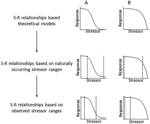
The trajectories of S-R relationships derived from field measurements may differ substantially from naturally occurring S-R relationships, which may in turn differ from S-R relationships predicted from theoretical models. There are several possible explanations for such differences: (1) the ranges of stressor and/or response values that have been measured are limited compared to the naturally occurring ranges; (2) the naturally occurring ranges are limited compared to those in the domain of the theoretical model; and (3) the underlying theoretical model is incorrect. The first two cases produce truncated versions of the underlying theoretical S-R relationship (Figure 2). In some cases, limited measurement ranges can result in observed S-R relationships that correspond to entirely different functions than the naturally occurring S-R relationships, e.g. observed S-R relationships that appear linear may be truncated portions of naturally occurring nonlinear relationships (Figure 2). The practical importance of these different inferences was demonstrated by a meta-analysis of published S-R relationships, which revealed a widespread tendency to fit linear relationships to sparse data, and nonlinear relationships to abundant data (Hunsicker et al. 2016). Incorrect inferences about naturally occurring S-R relationships can impede the development of effective environmental management strategies. Using the example on the right side of Figure 2, management strategies based on previously observed, linear S-R relationships cannot account for threshold behaviour if stressor levels increase in the future.

Figure 2. Sequences of S-R relationships from theoretical models to naturally occurring relationships (based on natural stressor ranges indicated by dashed lines), to observed relationships (based on monitoring over a limited stressor range indicated by dotted lines). A, Logistic S-R relationship appears to be logarithmic when observations exclude low stressor levels. B, Exponential S-R relationship appears to be linear when observations exclude high stressor levels.

In addition to the effects of limited data ranges, inferences about S-R relationships are affected by data scaling and transformations (e.g. normalising or linearising relationships). These data treatments can alter the trajectories of S-R relationships and obscure thresholds and domains of resistance (e.g. Stow and Cha 2013). A final source of variation in characterising S-R relationships is related to the use of single versus multiple sites. The most robust S-R relationships are based on data from individual sites at which paired stressor and response measurements have been made over the widest possible range of stressor levels. However, S-R relationships are often derived by compiling single pairs of stressor and response measurements from multiple sites and arranging them on a stressor gradient (e.g. Wagenhoff et al. 2011; Wang et al. 2014). In these ‘space-for-stress’ substitutions, each datum represents a different point on a site-specific S-R trajectory, and the response variables are influenced by site-specific conditions that can confound responses to the stressor (Johnson and Miyanishi 2008; MacNally et al. 2014; Capon et al. 2015). Advantages and disadvantages of the space-for-stress substitution approach are discussed further in the next section.

Using S-R relationships in prospective management of aquatic ecosystems

Early management strategies for aquatic ecosystems were predicated on the assumption that contaminant discharges are linearly and reversibly related to ecological responses (Guntenspergen and Gross 2014; Kelly et al. 2014). Strong support for this assumption came from observed increases in water clarity, macrophytes and other values as a function of decreasing nutrient concentrations following wastewater diversion from eutrophic lakes (e.g. Edmondson 1970; Ryding and Forsberg 1976; Soltero and Nichols 1984). The assumption of linearity was reflected in the widespread use of ‘pollution taxes’ that imposed fixed fees per unit of contaminant discharge, with no limit on the total allowable discharge and no allowance for nonlinear effects (Stavins and Whitehead 1992). However, the number of reports of nonlinear S-R relationships has increased rapidly (Walker and Meyers 2004; Rocha et al. 2015; Hunsicker et al. 2016). Many of the recent reports concern aquatic ecosystems that degraded rapidly when water-quality thresholds were exceeded, and a subset of those cases failed to recover in response to water-quality improvements (e.g. Schallenberg and Sorrell 2009; Kelly et al. 2015; Liu et al. 2015).

Threshold dynamics in aquatic ecosystems and the limited capacity of these systems to recover from degradation have led to recommendations for threshold-based environmental management (Kelly et al. 2014; Liu et al. 2015; Schallenberg et al. 2017). Threshold-based management is prospective because its aims are to forecast ecological thresholds in advance and prevent them from being crossed. Prospective management contrasts with retrospective or reactive management, which focuses on arresting degradation after it occurs and rehabilitating degraded ecosystems (Hobbs et al. 2011; Thom et al. 2016). Despite the widely-acknowledged need, few environmental agencies have made prospective management an explicit policy (Kelly et al. 2014).

Reliably forecasting ecological responses to stressors is one of the greatest challenges facing prospective management, and highly uncertain forecasts provide little incentive for management actions. Uncertainty about the proximity of a threshold means that degradation can commence with little or no warning, which limits or precludes preventative action. Uncertainty about predicted thresholds is exacerbated in situations where stochastic events cause degradation independently of stressor effects (Carpenter and Lathrop 2008; Pace et al. 2015). These potential problems have hampered forecasting ecological thresholds, although considerable effort has been expended on identifying thresholds after they occur (Andersen et al. 2009; Bestelmeyer et al. 2011; Toms and Villard 2015).

Despite the challenges, results from ecosystem experiments and some nascent prospective management programmes indicate that, given sufficient data and lead times, responses to increased stressor levels can be accurately forecasted and preventative actions can avert degradation (Carpenter et al. 2011; Kelly et al. 2015; Pace et al. 2017). An important attribute shared by these successful cases was the availability of monitoring data for characterising S-R relationships, predicting thresholds, setting management targets, and assessing management effectiveness.

Steps in prospective management

In the remainder of this section, we discuss four general steps for effective prospective management, distilled from recent contributions to the environmental management literature: (1) specify which S-R relationships are to be managed, based on high-priority response variables and their controlling stressors; (2) characterise S-R relationships and predict locations of stressor thresholds; (3) link management targets to predicted thresholds; and (4) implement adaptive management and prepare for rapid interventions to avoid breaching S-R thresholds. Each step requires monitoring data, and for many agencies, generating the data required for threshold-based management will require an increased investment in monitoring activities, or a redesign of current monitoring programmes, or both.

Step 1. Identify S-R relationships to be managed, based on high-priority response variables and their controlling stressors

The response variables in S-R relationships generally represent normative values such as human and ecological health and aesthetic quality (Ruiz-Frau et al. 2011; Tadaki et al. 2017). When normative values are qualitative (e.g. clear water, healthy ecosystems), quantitative indicators of these values are needed to develop continuously varying S-R relationships, and these indicators serve as response variables. The number of potential response variables far exceeds the capacities of most monitoring programmes, and criteria are needed to identify the variables that warrant monitoring. Criteria include importance to stakeholders, rarity (e.g. endangered species populations) and sensitivity to stressors. Metrics based on biotic community structure and taxonomic composition are common response variables as they tend to be sensitive to abiotic stresses such as nutrient enrichment and acidification (Schindler 1987; King and Baker 2010). Populations of habitat-forming species and keystone species are also common response variables, as they serve as surrogates for multiple dependent species (Selkoe et al. 2015).

The stressor variables most frequently used in S-R relationships for aquatic ecosystems are direct drivers of environmental degradation. These drivers include contaminants that originate from land use activities (e.g. nutrients, toxicants, pathogenic microbes) and physical habitat factors (e.g. fine sediment cover, dissolved oxygen). Indirect stressor variables (e.g. agricultural land cover, impervious land area, livestock density) are also used, as discussed in the preceding section.

Preliminary selections of stressor variables are often made using conceptual models of presumed stressor-response associations (Lindenmeyer and Likens 2009). When monitoring data are available, candidate stressor variables can be identified using statistical correlations with the selected response variables or with causal inference methods such as structural equation modelling (Irvine et al. 2015). When monitoring data are scarce, stressor-response associations may be identified using expert opinion and literature reviews (Tegler et al. 2001; Norris et al. 2011). A common aim of these approaches is to reduce the number of possible S-R relationships to the most informative set that minimises redundant variables.

Step 2. Characterise S-R relationships and forecast their trajectories, including thresholds

As noted above, S-R relationships are generally characterised retrospectively, after a stressor threshold has been exceeded. For prospective management, S-R trajectories and thresholds need to be predicted in advance. Four general approaches have been used to make these predictions: process-based modelling, statistical models based on space-for-stress substitutions, historical observations, and cross-site comparisons.

In the process-based modelling approach, S-R relationships are based on functions that represent the presumed causal relationships between the stressors and responses. One of the primary uses of process-based models in prospective management is for developing nutrient-load limits to prevent lake and estuary eutrophication (e.g. Trolle et al. 2008, 2014; Scavia et al. 2016; Jones et al. 2018). More widespread use of models to forecast S-R trajectories has been impeded by complex model structures and limited data for parameterisation and calibration (Oliver and Roy 2015). Despite the current impediments, the proficiency of model-based forecasting is certain to increase, for two reasons. First, the use of ensemble modelling (using multiple models to predict the same response) for more robust predictions is expanding rapidly (Nielsen et al. 2014; Janssen et al. 2015). Second, data generated by remote sensing, autonomous instruments and observation networks are growing at an unprecedented rate and data accessibility is increasing; these developments will reduce forecast uncertainty (Luo et al. 2011; Hamilton et al. 2015).

In the space-for-stress substitution approach, one-off measurements of stressor and response variables at multiple monitoring sites are arranged on a stressor gradient to produce an aggregate S-R relationship. With this approach, it is implicitly assumed that the aggregate relationship represents the trajectory at each measurement site and that the principal differences among sites are in stressor levels. In most applications, the aggregate S-R relationships are characterised using regressions or other curve-fitting methods, and thresholds in those relationships are estimated using breakpoint analysis tools (e.g. Trebitz 2012; Wang et al. 2014). The estimated thresholds are then used to propose stressor limits for management (e.g. nutrient criteria, maximum allowable contaminant loads). Advantages of the space-for-stress substitution approach include ease of interpolation and error estimation, and minimal time requirements, as there is no need for repeated sampling as stressor levels change at monitoring sites. However, this approach has two major shortcomings: instantaneous observations from multiple sites convey no information about site-specific trajectories; and stressor and response data in space-for-stress substitutions are usually log-transformed, which may linearise nonlinear relationships.

The historical observations approach is applicable for individual lakes and other sites where repeated cycles of threshold exceedance, degradation and recovery have occurred, and for which stressor and response data spanning the threshold events are available. For example, Swedish lakes monitored for > 30 years underwent repeated shifts between healthy (clear water, macrophyte dominance) and degraded (turbid water, phytoplankton dominance) states, partly in response to variable phosphorus loads (Hargeby et al. 2007). There was a two-fold difference in mean total phosphorus concentrations during turbid periods compared with clear periods; the threshold total phosphorus concentration beyond which the lakes shifted to the turbid state was estimated to be 30–55 μg L⁻¹. The historical approach is rarely used due to the perceived scarcity of suitable long-term monitoring data. However, concatenation of multiple short-term datasets and proxy variables can circumvent this problem (Wang et al. 2012). A second potential problem with this approach is that stressor thresholds may change over time due to progressive changes in other, interacting stressors. For example, climate warming is predicted to reduce the threshold nutrient levels beyond which planktonic cyanobacteria proliferate in shallow lakes (Wagner and Adrian 2009; Kosten et al. 2012).

In the cross-site comparison approach, S-R relationships for one or more sites that have crossed ecological thresholds are used to predict future thresholds at sites that are not yet degraded but otherwise comparable. In some cases, the predicted thresholds are based on generalised statistical S-R models; models of climate impacts on species distributions are examples of this approach (e.g. Araujo et al. 2005). More frequently, cross-site predictions are simply based on observations of the stressor levels at which degradation occurs in one or more comparable water bodies, without formal tests of transferability. For example, nitrogen loads corresponding to observed shifts in seven New Zealand coastal lagoons from macrophyte dominance to phytoplankton dominance were used to predict the threshold N load in a comparable lagoon that is vulnerable to a similar shift in the future (Schallenberg et al. 2017).

Of the four approaches summarised here, the historical observations and cross-site comparisons approaches are only useful for predicting the locations of thresholds on stressor gradients. For forecasting the trajectories of S-R relationships beyond the range of available data, extrapolation from models is required. Process-based models are better suited for extrapolation than empirical models such as those used in the space-for-stress substitution approach (Cuddington et al. 2013). Process based models rely on theory and governing equations that apply over broad stressor ranges and can include parameter values that have not yet been observed.

Each of the preceding approaches for predicting stressor thresholds is constrained by the availability of monitoring data and by uncertainty due to stochasticity, scale-interactions and slow-acting stressors such as legacy contaminants (Ascough et al. 2008; Tesoriero et al. 2013). To increase confidence, independent predictions of stressor threshold can be integrated using multiple-lines-of-evidence procedures (Smith and Tran 2010; Suter and Cormier 2011; Schallenberg et al. 2017). The lines of evidence may consist of two or more of the prediction methods summarised above, expert opinion, experimentation, or other methods. When there is wide divergence among predicted thresholds, they can be averaged or precautionary thresholds selected (e.g. the lowest of several predicted stressor thresholds). As an additional precaution, margins of safety can be used to trigger management actions prior to predicted thresholds, as discussed in Step 3 below.

To further reduce risks of incorrect forecasts and unforeseen thresholds, monitoring data can be used to track early warning indicators (EWIs) of impending thresholds (Scheffer et al. 2009, 2015; Wang et al. 2012). Most EWIs are based on temporal changes in skewness, autocorrelation and other statistical properties of response variable time-series. Observations of similar temporal patterns for different response variables, together with simplicity of analysis and potential applicability to complex systems, make statistical EWIs appealing tools (Carpenter and Brock 2006). However, EWIs are at an early stage of development; the types of thresholds for which EWIs are suitable or unsuitable is not yet clear, and recent tests of EWIs have revealed both failures to predict thresholds and false alarms (Litzow and Hunsicker 2016).

Step 3. Link management triggers to predicted thresholds

A management trigger (or ‘decision trigger’) is a point on an S-R curve at which management actions are initiated to prevent the stressor level from exceeding a pending threshold. (Martin et al. 2009; Schultz and Nie 2012). The primary function of a management trigger is to signal that the stressor level is sufficiently close to the threshold that failure to act is likely to result in exceedance. Management triggers may be set in terms of stressor variables (e.g. water quality ‘trigger values’; (Warne et al. 2014) or response variables (e.g. subcritical populations of endangered species; Schultz and Nie 2012). For brevity, we focus on management triggers in terms of stressor levels.

The difference between the stressor level associated with a management trigger and the stressor level corresponding to a predicted threshold is the ‘margin of safety’ (Scholes and Kruger 2011; Liu et al. 2015). Margins of safety are necessitated by uncertainty about stressor thresholds and the effectiveness of management actions, and by the time required for management actions to be implemented and for reductions in stressor levels to commence. These reductions range from days to decades, depending on the management action, administrative requirements (e.g. permitting), flushing rates in receiving environment, and levels of internal contaminant recycling, among other factors (e.g. Jeppesen et al. 2005). Cessation of contaminant discharges from point sources to receiving environments with short residence times may lead to rapid improvements in ecological state (e.g. Taylor et al. 2011). In contrast, effects of reductions in diffuse contaminant losses from land may be delayed by decades, due to the time required to deplete legacy contaminants that move slowly from source areas on land to aquatic receiving environments (Tesoriero et al. 2013; Morgenstern et al. 2015). If stressor levels are expected to continue increasing during these delays, management triggers need to be set at a lower stressor levels to compensate.

Step 4. Implement adaptive management and maintain capacity for rapid intervention

The term adaptive management is in wide use in environmental science and management and is associated with activities ranging from public participation in policy development to experimental tests of alternative management actions (Gregory et al. 2006; Allen and Gunderson 2011). Here, we use the term adaptive management to refer to a narrowly focused four-step process: (1) management actions are proposed to avert the exceedance of a forecasted S-R threshold; (2) the actions are carried out; (3) the effectiveness of the actions is evaluated by monitoring the stressor and response variables, and (4) the actions are modified as required (Williams 2011). The proposal-action-evaluation-modification sequence is iterated as necessary to forestall the threshold. As part of a broader prospective management strategy, adaptive management is initiated when the management trigger (discussed in Step 3) is reached.

Management actions intended to prevent threshold exceedance can be classed either as mitigations that reduce stressor levels (Figure 3A) or interventions that increase resistance to degradation (Figure 3B,C). Mitigations may be implemented on land (e.g. riparian buffers, stock exclusion, erosion control systems), where they reduce the loss of land-derived nutrients and other contaminants (McKergow et al. 2016; Fernandez 2017), or in the transport network linking land to aquatic receiving environments, where they reduce contaminant loading (e.g. treatment wetlands, alum additions to lake tributaries, diversion of sewage effluent; Rogers 2003; Burns et al. 2009; Tournebize et al. 2017).

Figure 3. Effects of mitigations and interventions on S-R relationships and resistance to stressors. A, Mitigations and interventions that reduce contaminant loads reduce stressor levels. B, Interventions that increase resistance shift the S-R relationship to the right from the pre-intervention relationship (dashed line). C, Interventions that either reduce adverse effects or restore values both shift the S-R relationship upwards from the pre-intervention relationship (dashed line).

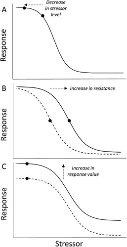
In contrast to mitigations, interventions are implemented in the aquatic receiving environments of concern. Interventions operate in two general ways: reducing contaminant levels in the receiving environment (e.g. lake and estuary flushing, in-lake alum application and sediment capping; Özkundakci et al. 2010; Elliott et al. 2016), and increasing resistance to degradation (e.g. shading lake beds to reduce macrophyte proliferations; Schooler 2008). With regard to S-R relationships, mitigations and interventions that reduce contaminant levels shift the stressor level to the left (Figure 3A). In contrast, interventions that increase resistance to degradation extend the domain of resistance and shift stressor thresholds to the right (Figure 3B).

The beneficial effects of some interventions (e.g. sediment-capping, additions of phosphorus-binding agents, river flushing flows) can be short-lived, particularly in cases where external stressor levels such as contaminant loading and flow depletion remain high (Robinson et al. 2004, Gibbs et al. 2011; Huser et al. 2016). In these cases, the interventions need to be repeated to prevent degradation, or the interventions need to be accompanied by management actions that increase resistance to degradation. As noted above, aquatic ecosystems have natural stabilising feedback mechanisms that confer resistance to degradation. This natural resistance can be enhanced using targeted interventions; examples of interventions used in conjunction with natural feedback mechanisms in lakes are summarised in Table 1.

The two general types of interventions discussed here are associated with prospective management; i.e. they are intended to reduce the risk of exceeding thresholds. Other types of in situ interventions are intended to reduce adverse effects after they have occurred (e.g. lake biocontrol; Burns et al. 2014), and to replace lost or decimated ecological components (e.g. replanting lake macrophytes; Qiu et al. 2001). These retrospective interventions are not covered in the following discussion.

Under the prevailing conditions of uncertainty about S-R trajectories, adaptive management is best applied as a tiered process in which monitoring intensity and investments in management actions increase with increasing proximity to the predicted threshold (Beeden et al. 2012; Selkoe et al. 2015). When a stressor level is far below a management trigger, monitoring may be limited to periodic surveys. As the stressor level approaches the margin of safety, monitoring increases in frequency and initial management actions are implemented. Subsequent monitoring is used to assess the effectiveness of the management actions and to inform modifications in those actions as necessary. Combining a precautionary margin of safety and tiered monitoring and management is intended to control costs while ensuring that there is sufficient time to trial different actions until effective actions are identified. Several frameworks have been developed to help design and operate tiered monitoring and management strategies (e.g. Kingsford et al. 2011; McLoughlin et al. 2011).

The use of tiered adaptive management presumes that there is sufficient time for multiple iterations of the management proposal-action-evaluation-modification sequence. However, threshold exceedance can occur at stressor levels well below the predicted levels (e.g. Sasaki et al. 2015; Bertani et al. 2016). In these cases, premature threshold breaches were attributed to stochastic variation in stressor levels or abrupt disturbances (e.g. disease outbreaks, extreme weather events) that intensified the stressor effects. Combining risk-management strategies with tiered adaptive management can help managers reduce risks posed by stochastic variation and disturbances. One such strategy is ‘ecosystem resilience-building’, i.e. increasing natural resistance (Carpenter et al. 2012; Sasaki et al. 2015). Ecosystem resilience-building generally corresponds with the interventions listed in Table 1. A second risk-management strategy is a ‘rapid response system’, which is activated when disturbances occur that threaten to cause threshold breaches. For example, the risk that diseases and biological invasions will trigger or accelerate ecological degradation can be reduced by rapid eradication (Locke and Hanson 2009; Beric and MacIsaac 2015). To date, few rapid-response strategies have been explicitly linked to threshold responses to anthropogenic stressors. However, the need for such links is clear, based on reports of unanticipated threshold breaches.

Adaptive management, resilience-building and rapid-response capability are not mutually exclusive management strategies; large-scale environmental management programmes can incorporate all three. For example, programmes incorporating forecasting, adaptive management and intervention, impact mitigation (i.e. resilience-building) and rapid-response capability have been recommended for managing aquatic disease epidemics (Groner et al. 2016).

Concluding remarks

Prospective management of aquatic ecosystems presents many challenges and does not ensure that ecological degradation will be prevented. Uncertainty in forecasting and in management effectiveness precludes such assurance, but it does not prevent agencies from initiating prospective management strategies. Knowledge uncertainty can be reduced through continual monitoring and research. The implications of uncertainty can be identified through model sensitivity analyses and scenario testing (e.g. Arhonditsis and Brett 2005). And prospective management can commence without delay despite high uncertainty by employing adaptive management and precautionary margins of safety.

Ecological forecasting has been criticised because it relies on models with limited proficiency (Coreau et al. 2009). In turn, the risk of inaccurate forecasts has led to calls to delay their use for prospective management until forecasting skill increases (Dietze et al. 2018). However, delaying management actions while forecasts improve is not necessary or beneficial. Management actions must be taken in the present time, with or without input from forecasts. It is better to inform these decisions with forecasts of variable certainty (accompanied by characterisations of the uncertainty), then to withhold information. Margins of safety can then be adjusted to meet different levels of uncertainty. Providing early forecasts to managers is particularly important when S-R relationships are predicted to be nonlinear; in these cases, a lack of awareness incurs a high risk of abrupt, uncontrollable degradation (Martin et al. 2009).

The scope of this paper was limited to monotonic responses to single stressors due to the shortage of information and tools for prospectively managing multiple stressor situations. Despite the challenges, forecasting the effects of multiple stressors is a management imperative. Virtually all aquatic ecosystems are exposed to multiple stressors; even remote ecosystems are exposed to multiple stressors associated with global changes such as rising water temperature, acidification and atmospheric contaminant deposition (Hobbs WO et al. 2011). In developed catchments, global-stressors co-occur with local stressors such as invasive species and nutrient enrichment (Brown et al. 2013; Lawrence et al. 2014; Jackson et al. 2016).

Systematic approaches have been developed to evaluate multiple-stressor-response relationships (e.g. Menzie et al. 2007; Feld et al. 2016). In general, these approaches comprise: (1) reducing large numbers of potential stressors to a manageable set of the most influential (and least intercorrelated) stressors; (2) characterising the effects of individual stressors and ranking the stressors by effect size; and (3) characterising combined effects of the stressors, including interactions (e.g. synergistic, multiplicative, antagonistic). Recent advances in multiple stressors research include extrapolation from empirical data about combinations of stressors to novel combinations, and improvements in the null models used to test for interactions (Altenburger and Greco 2009; Schäfer and Piggott 2018). However, these advances do not address the principal need for prospective management, which is forecasting responses to multiple stressors beyond the range of observations, including thresholds in individual stressors. Ecological forecasting for multiple-stressor situations is at an early developmental stage and has been impeded by the limited capacity to predict responses to stressor interactions and to account for mediating factors such as species interactions (Harley et al. 2017). Empirical studies of the effects of multiple stressors on threshold levels of individual stressors are very rare (Hewitt et al. 2016). As with single-stressor S-R relationships, published reports of multiple stressor S-R relationships often lack strong evidence of threshold behaviour (Griffen et al. 2016). In view of these methodological and knowledge gaps and high levels of uncertainty, prospective management for aquatic ecosystems exposed to multiple stressors should be flexible (i.e. capable of shifting the target of management actions from one stressor to another), precautionary (i.e. initiated at stressor levels well below predicted thresholds), and benign (i.e. likely to have beneficial effects even if forecasted responses to multiple stressors prove incorrect (Lawler et al. 2010).

With the exception of marine fisheries management, prospective management programmes for aquatic ecosystems have minimal track records. Prospective management can lead to conflicts between socio-economic activities and management actions (e.g. between land use intensification and reduced contaminant loading). The short-term constraints on socio-economic activities may be greater under prospective management compared to reactive management, although the long-term costs may be lower (Carpenter et al. 1999; Abell et al. 2011). These issues suggest that prospective management programmes will be slow to build track records of success and slow to gain support from affected stakeholders. Despite the challenges, we contend that prospective management is a logical successor to current strategies for managing aquatic ecosystems, and particularly to reactive management that responds to degradation after it occurs. Efforts to restore degraded ecosystems by reducing stressor levels often fail due to stabilising feedback, and managers must resort to remedial interventions (e.g. replanting macrophytes) to circumvent that feedback (Hobbs et al. 2011; Nyström et al. 2012; Bennion et al. 2015). In turn, the benefits of remedial interventions are often short-lived (e.g. Søndergaard et al. 2007; Tanner et al. 2010). Prospective, threshold-based management offers a promising alternative to these cases.

Acknowledgements

We thank B. Dudley and two anonymous referees for helpful reviews.

Disclosure statement

No potential conflict of interest was reported by the authors.

Additional information

Funding

This work was supported by Our Land and Water National Science Challenge, Ministry of Business, Innovation and Employment [grant number C10X1507] and the Lake Resilience programme (Ministry of Business, Innovation and Employment contract UOWX1503).

References

- Abell JM, Hamilton DP, Paterson J. 2011. Reducing the external environmental costs of pastoral farming in New Zealand: experiences from the Te Arawa lakes, Rotorua. Australas J Env Man. 18:139–154.
- Abell JM, Özkundakci D, Hamilton DP, Jones JR. 2012. Latitudinal variation in nutrient stoichiometry and chlorophyll-nutrient relationships in lakes: a global study. Fund Appl Limnol. 181:1–14.
- Adams SM. 2003. Establishing causality between environmental stressors and effects on aquatic ecosystems. Hum Ecol Risk Assess. 9:17–35.
- Allen CR, Gunderson LH. 2011. Pathology and failure in the design and implementation of adaptive management. J Environ Manage. 92:1379–1384.
- Altenburger R, Greco WR. 2009. Extrapolation concepts for dealing with multiple contamination in environmental risk assessment. Integr Environ Assess Manag. 5:62–68.
- Andersen T, Carstensen J, Hernandez-Garcia E, Duarte CM. 2009. Ecological regime shifts: approaches to identification. Trends Ecol Evol. 24:49–57.
- Anttila S, Ketola M, Kuoppamäki K, Kairesalo T. 2013. Identification of a biomanipulation-driven regime shift in Lake Vesijärvi: implications for lake management. Freshwater Biol. 58:1494–1502.
- Araujo MB, Pearson RG, Thuiller W, Erhard M. 2005. Validation of species–climate impact models under climate change. Global Change Biol. 11:1504–1513.
- Arhonditsis GB, Brett MT. 2005. Eutrophication model for Lake Washington (USA): part I. Model description and sensitivity analysis. Ecol Model. 187:140–178.
- Ascough JC, Maier HR, Ravalico JK, Strudley MW. 2008. Future research challenges for incorporation of uncertainty in environmental and ecological decision-making. Ecol Model. 219:383–399.
- Beeden R, Maynard JA, Marshall PA, Heron SF, Willis BL. 2012. A framework for responding to coral disease outbreaks that facilitates adaptive management. Environ Manage. 49:1–13.
- Beisner BE, Haydon DT, Cuddington K. 2003. Alternative stable states in ecology. Front Ecol Environ. 1:376–382.
- Bennion H, Simpson GL, Goldsmith BJ. 2015. Assessing degradation and recovery pathways in lakes impacted by eutrophication using the sediment record. Front Ecol Evol. 3:1–20.
- Beric B, MacIsaac HJ. 2015. Determinants of rapid response success for alien invasive species in aquatic ecosystems. Biol Invasions. 17:3327–3335.
- Bertani I, Primicerio R, Rossetti G. 2016. Extreme climatic event triggers a lake regime shift that propagates across multiple trophic levels. Ecosystems. 19:16–31.
- Bestelmeyer BT, Ellison AM, Fraser WR, Gorman KB, Holbrook SJ, Laney CM, Ohman MD, Peters DP, Pillsbury FC, Rassweiler A, Schmitt RJ. 2011. Analysis of abrupt transitions in ecological systems. Ecosphere. 2:1–26.
- Blindow I, Andersson G, Hargeby A, Johansson S. 1993. Long-term pattern of alternative stable states in two shallow eutrophic lakes. Freshwater Biol. 30:159–167.
- Bormans M, Jancula D, Marsalek B. 2016. Controlling internal phosphorus loading in lakes by physical methods to reduce cyanobacterial blooms: a review. Aquat Ecol. 50:407–422.
- Brown CJ, Saunders MI, Possingham HP, Richardson AJ. 2013. Managing for interactions between local and global stressors of ecosystems. PloS one. 8(6):e65765.
- Burns CW, Schallenberg M, Verburg P. 2014. Potential use of classical biomanipulation to improve water quality in New Zealand lakes: a re-evaluation. N Z J Mar Freshwat Res. 48:127–138.
- Burns N, McIntosh J, Scholes P. 2009. Managing the lakes of the Rotorua district, New Zealand. Lake Reserv Manage. 25:284–296.
- Capon SJ, Lynch AJJ, Bond N, Chessman BC, Davis J, Davidson N, Finlayson M, Gell PA, Hohnberg D, Humphrey C, Kingsford RT. 2015. Regime shifts, thresholds and multiple stable states in freshwater ecosystems; a critical appraisal of the evidence. Sci Total Environ. 534:122–130.
- Carpenter SR, Arrow KJ, Barrett S, Biggs R, Brock WA, Crépin AS, Engström G, Folke C, Hughes TP, Kautsky N, Li CZ. 2012. General resilience to cope with extreme events. Sustainability. 4:3248–3259.
- Carpenter SR, Brock WA. 2006. Rising variance: a leading indicator of ecological transition. Ecol Lett. 9:308–315.
- Carpenter SR, Cole JJ, Pace ML, Batt R, Brock WA, Cline T, Coloso J, Hodgson JR, Kitchell JF, Seekell DA, Smith L. 2011. Early warnings of regime shifts: a whole-ecosystem experiment. Science. 332(6033):1079–1082.
- Carpenter SR, Lathrop RC. 2008. Probabilistic estimate of a threshold for eutrophication. Ecosystems. 11:601–613.
- Carpenter SR, Ludwig D, Brock WA. 1999. Management of eutrophication for lakes subject to potentially irreversible change. Ecol Appl. 9:751–771.
- Clements WH, Vieira NK, Church SE. 2010. Quantifying restoration success and recovery in a metal-polluted stream: a 17-year assessment of physicochemical and biological responses. J Appl Ecol. 47:899–910.
- Coats R, Larsen M, Heyvaert A, Thomas J, Luck M, Reuter J. 2008. Nutrient and sediment production, watershed characteristics, and land use in the Tahoe Basin, California-Nevada. J Am Water Resour Assoc. 44:754–770.
- Coreau A, Pinay G, Thompson JD, Cheptou PO, Mermet L. 2009. The rise of research on futures in ecology: rebalancing scenarios and predictions. Ecol Lett. 12:1277–1286.
- Cuddington K, Fortin MJ, Gerber LR, Hastings A, Liebhold A, O’connor M, Ray C. 2013. Process-based models are required to manage ecological systems in a changing world. Ecosphere. 4:1–12.
- Darling ES, Côté IM. 2008. Quantifying the evidence for ecological synergies. Ecol Lett. 11:1278–1286.
- Davis J, Sim L, Chambers J. 2010. Multiple stressors and regime shifts in shallow aquatic ecosystems in antipodean landscapes. Freshwater Biol. 55:5–18.
- Dietze MC. 2017. Ecological forecasting. Princeton, NJ: Princeton University Press.
- Dietze MC, Fox A, Beck-Johnson LM, Betancourt JL, Hooten MB, Jarnevich CS, Keitt TH, Kenney MA, Laney CM, Larsen LG, Loescher HW. 2018. Iterative near-term ecological forecasting: needs, opportunities, and challenges. Proc Natl Acad Sci. p201710231.
- Edmondson WT. 1970. Phosphorus, nitrogen, and algae in Lake Washington after diversion of sewage. Science. 169:690–691.
- Elliott M, Burdon D, Hemingway K, Apitz S. 2007. Estuarine, coastal and marine ecosystem restoration: confusing management and science – A revision of concepts. Estuar Coast Shelf Sci. 74:349–366.
- Elliott M, Mander L, Mazik K, Simenstad C, Valesini F, Whitfield A, Wolanski E. 2016. Ecoengineering with ecohydrology: successes and failures in estuarine restoration. Estuar Coast Shelf Sci. 176:12–35.
- Feld CK, Segurado P, Gutiérrez-Cánovas C. 2016. Analysing the impact of multiple stressors in aquatic biomonitoring data: a ‘cookbook’with applications in R. Sci Total Environ. 573:1320–1339.
- Fernandez MA. 2017. Adoption of erosion management practices in New Zealand. Land Use Pol. 63:236–245.
- Filstrup CT, Wagner T, Soranno PA, Stanley EH, Stow CA, Webster KE, Downing JA. 2014. Regional variability among nonlinear chlorophyll-phosphorus relationships in lakes. Limnol Oceanogr. 59:1691–1703.
- Flynn KF, Suplee MW, Chapra SC, Tao H. 2015. Model-based nitrogen and phosphorus (nutrient) criteria for large temperate rivers: 1. Model development and application. J Am Water Resour Assoc. 51:421–446.
- Folke C, Carpenter S, Walker B, Scheffer M, Elmqvist T, Gunderson L, Holling CS. 2004. Regime shifts, resilience, and biodiversity in ecosystem management. Annu Rev Ecol Evol Syst. 35:557–581.
- Frost TM, Carpenter SR, Ives AR, Kratz T. 1995. Species compensation and complementarity in ecosystem function. In: Jones C, Lawton J, editors. Linking species and ecosystems. London, England: Chapman and Hall; p. 224–239.
- Gergel SE, Turner MG, Miller JR, Melack JM, Stanley EH. 2002. Landscape indicators of human impacts to riverine systems. Aq Sci. 64:118–128.
- Ghedini G, Connell SD. 2016. Organismal homeostasis buffers the effects of abiotic change on community dynamics. Ecology. 97:2671–2679.
- Gibbs MM, Hickey CW, Özkundakci D. 2011. Sustainability assessment and comparison of efficacy of four P-inactivation agents for managing internal phosphorus loads in lakes: sediment incubations. Hydrobiologia. 658:253–275.
- Gregory R, Ohlson D, Arvai J. 2006. Deconstructing adaptive management: criteria for applications to environmental management. Ecol Appl. 16:2411–2425.
- Griffen BD, Belgrad BA, Cannizzo ZJ, Knotts ER, Hancock ER. 2016. Rethinking our approach to multiple stressor studies in marine environments. Mar Ecol Progr Ser. 543:273–281.
- Groffman P, Baron J, Blett T, Gold A, Goodman I, Gundersen L, Levinson BM, Palmer MA, Paerl HW, Peterson GD, et al. 2006. Ecological thresholds: the key to successful environmental management or an important concept with no practical application? Ecosystems. 9:1–13.
- Groner ML, Maynard J, Breyta R, Carnegie RB, Dobson A, Friedman CS, Froelich B, Garren M, Gulland FM, Heron SF, Noble RT. 2016. Managing marine disease emergencies in an era of rapid change. Philos Trans R Soc Lond B. 371:20150364.
- Guntenspergen GR, Gross J. 2014. Threshold concepts: implications for the management of natural resources. In: Guntenspergen GR, editor. Application of threshold concepts in natural resource decision making. New York: Springer; p. 1–7.
- Halpern BS, Fujita R. 2013. Assumptions, challenges, and future directions in cumulative impact analysis. Ecosphere. 4:1–11.
- Hamilton DP, Carey CC, Arvola L, Arzberger P, Brewer C, Cole JJ, Gaiser E, Hanson PC, Ibelings BW, Jennings E, Kratz TK. 2015. A Global Lake Ecological Observatory Network (GLEON) for synthesising high-frequency sensor data for validation of deterministic ecological models. Inland Waters. 5:49–56.
- Hargeby A, Blindow I, Andersson G. 2007. Long-term patterns of shifts between clear and turbid states in Lake Krankesjön and Lake Tåkern. Ecosystems. 10:29–36.
- Harley CD, Connell SD, Doubleday ZA, Kelaher B, Russell BD, Sarà G, Helmuth B. 2017. Conceptualizing ecosystem tipping points within a physiological framework. Ecol Evol. 7:6035–6045.
- Hewitt JE, Ellis JI, Thrush SF. 2016. Multiple stressors, nonlinear effects and the implications of climate change impacts on marine coastal ecosystems. Global Change Biol. 22:2665–2675.
- Hickey CW, Gibbs MM. 2009. Lake sediment phosphorus release management: decision support and risk assessment framework. N Z J Mar Freshwat Res. 43:819–856.
- Hilt S, Gross EM, Hupfer M, Morosheid H, Mählmann J, Melzer A, Poltz J, Sandrock S, Scharf E-M, Schneider S, van den Weyer K. 2006. Restoration of submerged vegetation in shallow eutrophic lakes: a guideline and state of the art in Germany. Limnologica. 36:155–171.
- Hobbs RJ, Hallett LM, Ehrlich PR, Mooney H. 2011. Intervention ecology: applying ecological science in the twenty-first century. BioScience. 61:442–450.
- Hobbs WO, Vinebrooke RD, Wolfe AP. 2011. Biogeochemical responses of two alpine lakes to climate change and atmospheric deposition, Jasper and Banff National parks, Canadian Rocky Mountains. Can J Fish Aq Sci. 68:1480–1494.
- Hodgsen D, McDonald JL, Hosken DJ. 2015. What do you mean, ‘resilient’? Trends Ecol Evol. 30:503–506.
- Holling CS. 1973. Resilience and stability of ecological systems. Annu Rev Ecol Syst. 4:1–23.
- Holling CS. 1996. Engineering resilience versus ecological resilience. In: Schulze PC, editor. Engineering within ecological constraints. Washington, DC: National Academy Press; p. 31–44.
- Hughes TP, Barnes ML, Bellwood DR, Cinner JE, Cumming GS, Jackson JB, Kleypas J, Van De Leemput IA, Lough JM, Morrison TH, Palumbi SR. 2017. Coral reefs in the Anthropocene. Nature. 546:82–90.
- Hughes TP, Reed DC, Boyle MJ. 1987. Herbivory on coral reefs: community structure following mass mortalities of sea urchins. J Exp Mar Biol Ecol. 113:39–59.
- Hunsicker ME, Kappel CV, Selkoe KA, Halpern BS, Scarborough C, Mease L, Amrhein A. 2016. Characterizing driver–response relationships in marine pelagic ecosystems for improved ocean management. Ecol Appl. 26:651–663.
- Huser BJ, Egemose S, Harper H, Hupfer M, Jensen H, Pilgrim KM, Reitzel K, Rydin E, Futte M. 2016. Longevity and effectiveness of aluminum addition to reduce sediment phosphorus release and restore lake water quality. Water Res. 97:122–132.
- Irvine KM, Miller SW, Al-Chokhachy RK, Archer EK, Roper BB, Kershner JL. 2015. Empirical evaluation of the conceptual model underpinning a regional aquatic long-term monitoring program using causal modelling. Ecol Indic. 50:8–23.
- Jackson MC, Loewen CJ, Vinebrooke RD, Chimimba CT. 2016. Net effects of multiple stressors in freshwater ecosystems: a meta-analysis. Global Change Biol. 22:180–189.
- Janssen AB, Arhonditsis GB, Beusen A, Bolding K, Bruce L, Bruggeman J, Couture RM, Downing AS, Elliott JA, Frassl MA, Gal G. 2015. Exploring, exploiting and evolving diversity of aquatic ecosystem models: a community perspective. Aq Ecol. 49:513–548.
- Jeppesen E, Søndergaard M, Jensen JP, Havens KE, Anneville O, Carvalho L, Coveney MF, Deneke R, Dokulil MT, Foy BOB, Gerdeaux D. 2005. Lake responses to reduced nutrient loading–an analysis of contemporary long-term data from 35 case studies. Freshwater Biol. 50:1747–1771.
- Johnson A, Miyanishi K. 2008. Testing the assumptions of chronosequences in succession. Ecol Lett. 11:419–431.
- Jones HF, Özkundakci D, McBride CG, Pilditch CA, Allan MG, Hamilton DP. 2018. Modelling interactive effects of multiple disturbances on a coastal lake ecosystem: implications for management. J Environ Manage. 207:444–455.
- Kelly RP, Erickson AL, Mease LA. 2014. How not to fall off a cliff, or, using tipping points to improve environmental management. Ecol Law Quart. 41:843–885.
- Kelly RP, Erickson AL, Mease LA, Battista W, Kittinger JN, Fujita R. 2015. Embracing thresholds for better environmental management. Phil Trans R Soc London B: Biol Sci. 370:20130276.
- Kemp WM, Testa JM, Conley DJ, Gilbert D, Hagy JD. 2009. Temporal responses of coastal hypoxia to nutrient loading and physical controls. Biogeosciences. 6:2985–3008.
- King RS, Baker ME. 2010. Considerations for analyzing ecological community thresholds in response to anthropogenic environmental gradients. J N Am Benthol Soc. 29:998–1008.
- Kingsford RT, Biggs HC, Pollard SR. 2011. Strategic adaptive management in freshwater protected areas and their rivers. Biol Conserv. 144:1194–1203.
- Kopf RK, Finlayson CM, Humphries P, Sims NC, Hladyz S. 2015. Anthropocene baselines: assessing change and managing biodiversity in human-dominated aquatic ecosystems. BioScience. 65:798–811.
- Kosten S, Huszar VL, Bécares E, Costa LS, Van Donk E, Hansson LA, Jeppesen E, Kruk C, Lacerot G, Mazzeo N, De Meester L. 2012. Warmer climates boost cyanobacterial dominance in shallow lakes. Global Change Biol. 18:118–126.
- Lake PS, Bond N, Reich P. 2007. Linking ecological theory with stream restoration. Freshwater Biol. 52:597–615.
- Lawler JJ, Tear TH, Pyke C, Shaw MR, Gonzalez P, Kareiva P, Hansen L, Hannah L, Klausmeyer K, Aldous A, Bienz C. 2010. Resource management in a changing and uncertain climate. Front Ecol Environ. 8:35–43.
- Lawrence DJ, Stewart-Koster B, Olden JD, Ruesch AS, Torgersen CE, Lawler JJ, Butcher DP, Crown JK. 2014. The interactive effects of climate change, riparian management, and a nonnative predator on stream-rearing salmon. Ecol Appl. 24:895–912.
- Lewison R, Hobday AJ, Maxwell S, Hazen E, Hartog JR, Dunn DC, Briscoe D, Fossette S, O’keefe CE, Barnes M, Abecassis M. 2015. Dynamic ocean management: identifying the critical ingredients of dynamic approaches to ocean resource management. BioScience. 65:486–498.
- Lindenmeyer DB, Likens GE. 2009. Adaptive monitoring: a new paradigm for long-term research and monitoring. Trends Ecol Evol. 24:482–486.
- Litzow MA, Hunsicker ME. 2016. Early warning signals, nonlinearity, and signs of hysteresis in real ecosystems. Ecosphere. 7(12):e01614. doi:10.1002/ecs2.1614.
- Liu J, Kattel G, Arp HPH, Yang H. 2015. Towards threshold-based management of freshwater ecosystems in the context of climate change. Ecol Model. 318:265–274.
- Locke A, Hanson JM. 2009. Rapid response to nonindigenous species. 3. A proposed framework. Aq Invasions. 4:259–273.
- Lundgren VM, Roelke DL, Grover JP, Brooks BW, Prosser KN, Scott WC, Laws CA, Umphres GD. 2013. Interplay between ambient surface water mixing and manipulated hydraulic flushing: implications for harmful algal bloom mitigation. Ecol Eng. 60:289–298.
- Luo Y, Ogle K, Tucker C, Fei S, Gao C, LaDeau S, Clark JS, Schimel DS. 2011. Ecological forecasting and data assimilation in a data-rich era. Ecol Appl. 21:1429–1442.
- MacNally R, Albano C, Fleishman E. 2014. A scrutiny of the evidence for pressure-induced state shifts in estuarine and nearshore ecosystems. Austral Ecol. 39:898–906.
- Martin J, Runge MC, Nichols JD, Lubow BC, Kendall WL. 2009. Structured decision making as a conceptual framework to identify thresholds for conservation and management. Ecol Appl. 19:1079–1090.
- McKergow LA, Matheson FE, Quinn JM. 2016. Riparian management: a restoration tool for New Zealand streams. Ecol Manag Restor. 17:218–227.
- McLoughlin CA, Deacon A, Sithole H, Gyedu-Ababio T. 2011. History, rationale, and lessons learned: thresholds of potential concern in Kruger National Park river adaptive management. Koedoe. 53:69–95.
- Menzie CA, MacDonell MM, Mumtaz M. 2007. A phased approach for assessing combined effects from multiple stressors. Environ Health Persp. 115:807–816.
- Merill L, Tonjes DJ. 2014. A review of the hyporheic zone, stream restoration, and means to enhance denitrification. Crit Rev Env Sci Tec. 44:2337–2379.
- Morgenstern U, Daughney CJ, Leonard G, Gordon D, Donath FM, Reeves R. 2015. Using groundwater age and hydrochemistry to understand sources and dynamics of nutrient contamination through the catchment into Lake Rotorua, New Zealand. Hydrol Earth Syst Sci. 19:803–822.
- Mouquet N, Lagadeuc Y, Devictor V, Doyen L, Duputié A, Eveillard D, Faure D, Garnier E, Gimenez O, Huneman P, Jabot F. 2015. Predictive ecology in a changing world. J Appl Ecol. 52:1293–1310.
- Nichols SJ, Peat M, Webb JA. 2017. Challenges for evidence-based environmental management: what is acceptable and sufficient evidence of causation? Freshwater Sci. 36:240–249.
- Nielsen A, Trolle D, Bjerring R, Søndergaard M, Olesen JE, Janse JH, Mooij WM, Jeppesen E. 2014. Effects of climate and nutrient load on the water quality of shallow lakes assessed through ensemble runs by PCLake. Ecol Appl. 24:1926–1944.
- Norris RH, Webb JA, Nichols SJ, Stewardson MJ, Harrison ET. 2011. Analyzing cause and effect in environmental assessments: using weighted evidence from the literature. Freshwater Sci. 31:5–21.
- Nyström M, Norström AV, Blenckner T, de la Torre-Castro M, Eklöf JS, Folke C, Österblom H, Steneck RS, Thyresson M, Troell M. 2012. Confronting feedbacks of degraded marine ecosystems. Ecosystems. 15:695–710.
- Oliver TH, Roy DB. 2015. The pitfalls of ecological forecasting. Biol J Linn Soc. 115:767–778.
- Özkundakci D, Hamilton DP, Scholes P. 2010. Effect of intensive catchment and in-lake restoration procedures on phosphorus concentrations in a eutrophic lake. Ecol Eng. 36:396–405.
- Pace ML, Batt RD, Buelo CD, Carpenter SR, Cole JJ, Kurtzweil JT, Wilkinson GM. 2017. Reversal of a cyanobacterial bloom in response to early warnings. Proc Natl Acad Sci. 114:352–357.
- Pace ML, Carpenter SR, Cole JJ. 2015. With and without warning: managing ecosystems in a changing world. Front Ecol Environ. 13:460–467.
- Petchey OL, Pontarp M, Massie TM, Kéfi S, Ozgul A, Weilenmann M, Palamara GM, Altermatt F, Matthews B, Levine JM, Childs DZ. 2015. The ecological forecast horizon, and examples of its uses and determinants. Ecol Lett. 18:597–611.
- Petraitis PS, Dudgeon SR. 2004. Detection of alternative stable states in marine communities. J Exp Mar Biol Ecol. 300:343–371.
- Pierce SC, Kröger R, Pzeshki R. 2012. Managing artificially drained low-gradient agricultural headwaters for enhanced ecosystem functioning. Biology. 1:794–856.
- Qiu D, Wu Z, Liu B, Deng J, Fu G, He F. 2001. The restoration of aquatic macrophytes for improving water quality in a hypertrophic shallow lake in Hubei Province, China. Ecol Eng. 18:147–156.
- Reynolds CS. 1994. The ecological basis for the successful biomanipulation of aquatic communities. Arch Hydrobiol. 130:1–33.
- Rocha JC, Peterson GD, Biggs R. 2015. Regime shifts in the Anthropocene: drivers, risks, and resilience. PloS One. 10(8):e0134639.
- Rogers KM. 2003. Stable carbon and nitrogen isotope signatures indicate recovery of marine biota from sewage pollution at Moa Point, New Zealand. Mar Pollut Bull. 46:821–827.
- Rosenfeld JS. 2017. Developing flow–ecology relationships: implications of nonlinear biological responses for water management. Freshwater Biol. 62:1305–1324.
- Rowe DK, Champion PD. 1994. Biomanipulation of plants and fish to restore Lake Parkinson: a case study and its implications. In: Collier KJ, editor. Restoration of aquatic habitats. Wellington: Department of Conservation; p. 53–65.
- Ruiz-Frau A, Edwards-Jones G, Kaiser MJ. 2011. Mapping stakeholder values for coastal zone management. Mar Ecol Prog Ser. 434:239–249.
- Ryding SO, Forsberg C. 1976. Six polluted lakes: a preliminary evaluation of the treatment and recovery processes. Ambio. 5:151–156.
- Saar DA. 2002. Riparian livestock exclosure research in the western United States: a critique and some recommendations. Environ Manage. 30:516–526.
- Sasaki T, Furukawa T, Iwasaki Y, Seto M, Mori AS. 2015. Perspectives for ecosystem management based on ecosystem resilience and ecological thresholds against multiple and stochastic disturbances. Ecol Indic. 57:395–408.
- Scavia D, DePinto JV, Bertani I. 2016. A multi-model approach to evaluating target phosphorus loads for Lake Erie. J Great Lakes Res. 42:1139–1150.
- Schäfer RB, Piggott JJ. 2018. Advancing understanding and prediction in multiple stressor research through a mechanistic basis for null models. Global Change Biol. 24:1817–1826.
- Schallenberg M, Hamilton DP, Hicks AS, Robertson HA, Scarsbrook M, Robertson B, Wilson K, Whaanga D, Jones HFEE, Hamill K. 2017. Multiple lines of evidence determine robust nutrient load limits required to safeguard a threatened lake/lagoon system. N Z J Mar Freshwat Res. 51:78–95.
- Schallenberg M, Larned ST, Hayward S, Arbuckle C. 2010. Contrasting effects of managed opening regimes on water quality in two intermittently closed and open coastal lakes. Estuar Coast Shelf S. 86:587–597.
- Schallenberg M, Sorrell B. 2009. Regime shifts between clear and turbid water in New Zealand lakes: environmental correlates and implications for management and restoration. N Z J Mar Freshwat Res. 43:701–712.
- Scheffer M. 2004. The ecology of shallow lakes. Heidelberg: Springer-Verlag.
- Scheffer M, Bascompte J, Brock WA, Brovkin V, Carpenter SR, Dakos V, Held H, Van Nes EH, Rietkerk M, Sugihara G. 2009. Early-warning signals for critical transitions. Nature. 461:53–59.
- Scheffer M, Carpenter S, Foley JA, Folke C, Walker B. 2001. Catastrophic shifts in ecosystems. Nature. 413:591–596.
- Scheffer M, Carpenter SR, Dakos V, van Nes EH. 2015. Generic indicators of ecological resilience: inferring the chance of a critical transition. Annu Rev Ecol Evol Syst. 46:145–167.
- Schindler DW. 1987. Detecting ecosystem responses to anthropogenic stress. Can J Fish Aquat Sci. 44:s6–s25.
- Scholes RJ, Kruger JM. 2011. A framework for deriving and triggering thresholds for management intervention in uncertain, varying and time-lagged systems. Koedoe. 53:179–186.
- Schooler SS. 2008. Shade as a management tool for the invasive submerged macrophyte, Cabomba caroliniana. J Aquat Plant Manage. 46:168–171.
- Schröder A, Persson L, De Roos AM. 2005. Direct experimental evidence for alternative stable states: a review. Oikos. 110:3–19.
- Schultz C, Nie M. 2012. Decision-making triggers, adaptive management, and natural resources law and planning. Nat Resour J. 52:443–521.
- Selkoe KA, Blenckner T, Caldwell MR, Crowder LB, Erickson AL, Essington TE, Estes JA, Fujita RM, Halpern BS, Hunsicker ME, Kappel CV. 2015. Principles for managing marine ecosystems prone to tipping points. Ecosyst Health Sustainability. 1:1–18.
- Smith AJ, Tran CP. 2010. A weight-of-evidence approach to define nutrient criteria protective of aquatic life in large rivers. J N Am Benthol Soc. 29:875–891.
- Soltero RA, Nichols DG. 1984. The improved water quality of Long Lake following advanced wastewater treatment by the City of Spokane, Washington. Lake Reserv Manage. 1:395–404.
- Søndergaard M, Jeppesen E, Lauridsen TL, Skov C, Van Nes EH, Roijackers R, Lammens E, Portielje ROB. 2007. Lake restoration: successes, failures and long-term effects. J Appl Ecol. 44:1095–1105.
- Stavins RN, Whitehead BW. 1992. Pollution charges for environmental protection: a policy link between energy and environment. Annu Rev Energ Env. 17:187–210.
- Stow CA, Cha Y. 2013. Are chlorophyll a–total phosphorus correlations useful for inference and prediction? Environ Sci Technol. 47:3768–3773.
- Suter GW, Cormier SM. 2011. Why and how to combine evidence in environmental assessments: weighing evidence and building cases. Sci Total Environ. 409:1406–1417.
- Tadaki M, Sinner J, Chan KMA. 2017. Making sense of environmental values: a typology of concepts. Ecol Soc. 22(1):7.
- Tanner C, Hunter S, Reel J, Parham T, Naylor M, Karrh L, Busch K, Golden RR, Lewandowski M, Rybicki N, Schenk E. 2010. Evaluating a large-scale eelgrass restoration project in the Chesapeake Bay. Restor Ecol. 18:538–548.
- Taylor DI, Oviatt CA, Borkman DG. 2011. Non-linear responses of a coastal aquatic ecosystem to large decreases in nutrient and organic loadings. Estuar Coast. 34:745–757.
- Tegler B, Sharp M, Johnson MA. 2001. Ecological monitoring and assessment network’s proposed core monitoring variables: an early warning of environmental change. Environ Monit Assess. 67:29–55.
- Tesoriero AJ, Duff JH, Saad DA, Spahr NE, Wolock DM. 2013. Vulnerability of streams to legacy nitrate sources. Environ Sci Technol. 47:3623–3629.
- Testa JM, Clark JB, Dennison WC, Donovan EC, Fisher AW, Ni W, Parker M, Scavia D, Spitzer SE, Waldrop AM, Vargas V. 2017. Ecological forecasting and the science of hypoxia in chesapeake Bay. BioScience. 67:614–626.
- Thom R, Clair TS, Burns R, Anderson M. 2016. Adaptive management of large aquatic ecosystem recovery programs in the United States. J Environ Manage. 183:424–430.
- Toms JD, Villard MA. 2015. Threshold detection: matching statistical methodology to ecological questions and conservation planning objectives. Avian Conserv Ecol. 10(1):2.
- Tournebize J, Chaumont C, Mander Ü. 2017. Implications for constructed wetlands to mitigate nitrate and pesticide pollution in agricultural drained watersheds. Ecol Eng. 103:415–425.
- Trebitz AS. 2012. Deriving criteria-supporting benchmark values from empirical response relationships: comparison of statistical techniques and effect of log-transforming the nutrient variable. Freshwater Sci. 31:986–1002.
- Trolle D, Skovgaard H, Jeppesen E. 2008. The Water Framework Directive: setting the phosphorus loading target for a deep lake in Denmark using the 1D lake ecosystem model DYRESM–CAEDYM. Ecol Model. 219:138–152.
- Trolle D, Spigel B, Hamilton DP, Norton N, Sutherland D, Plew D, Allan MG. 2014. Application of a three-dimensional water quality model as a decision support tool for the management of land-use changes in the catchment of an oligotrophic lake. Environ Manage. 54:479–493.
- Van Geest GJ, Coops H, Scheffer M, van Nes EH. 2007. Long transients near the ghost of a stable state in eutrophic shallow lakes with fluctuating water levels. Ecosystems. 10:37–47.
- Visser PM, Ibelings BW, Bormans M, Huisman J. 2016. Artificial mixing to control cyanobacterial blooms: a review. Aq Ecol. 50:423–441.
- Wagenhoff A, Townsend CR, Phillips N, Matthaei CD. 2011. Subsidy-stress and multiple-stressor effects along gradients of deposited fine sediment and dissolved nutrients in a regional set of streams and rivers. Freshwater Biol. 56:1916–1936.
- Wagner C, Adrian R. 2009. Cyanobacteria dominance: quantifying the effects of climate change. Limnol Oceanogr. 54:2460–2468.
- Walker B, Meyers J. 2004. Thresholds in ecological and social–ecological systems: a developing database. Ecol Soc. 9(2):3.
- Wang H-J, Wang H-Z, Liang X-M, Wu S-K. 2014. Total phosphorus threshold for regime shifts are nearly equal in subtropical and temperate shallow lakes with moderate depths and areas. Freshwater Biol. 59:1659–1671.
- Wang R, Dearing JA, Langdon PG, Zhang E, Yang X, Dakos V, Scheffer M. 2012. Flickering gives early warning signals of a critical transition to a eutrophic lake state. Nature. 492:419–422.
- Warne MSJ, Batley GE, Braga O, Chapman JC, Fox DR, Hickey CW, Stauber JL, Van Dam R. 2014. Revisions to the derivation of the Australian and New Zealand guidelines for toxicants in fresh and marine waters. Environ Sci Pollut R. 21:51–60.
- Welch EB. 1981. The dilution/flushing technique in lake restoration. J Am Water Resour Assoc. 17:558–564.
- Williams BK. 2011. Adaptive management of natural resources – framework and issues. J Environ Manage. 92:1346–1353.
- Wu F, Mu Y, Chang H, Zhao X, Giesy JP, Wu KB. 2012. Predicting water quality criteria for protecting aquatic life from physicochemical properties of metals or metalloids. Environ Sci Technol. 47:446–453.
- Yeh N, Yeh P, Chang YH. 2015. Artificial floating islands for environmental improvement. Renew Sust Energ Rev. 47:616–622.
- Zhao L, Li Y, Zou R, He B, Zhu X, Liu Y, Wang J, Zhu Y. 2013. A three-dimensional water quality modeling approach for exploring the eutrophication responses to load reduction scenarios in Lake Yilong (China). Environ Pollut. 177:13–21.