The role of wind and buoyancy forcing on mixed layer depths and productivity on the Chatham Rise from ocean glider and ship-based observations

ABSTRACT

The Subtropical Front (STF) and associated biological productivity are topographically locked to the Chatham Rise. Year-to-year differences of upper ocean dynamics and associated responses of phytoplankton are valuable for understanding variability in fisheries biomass as well as providing new knowledge of environmental condition for potential seabed mining in this keystone ecosystem. In-situ observations collected over three consecutive years are used to examine the oceanographic variability on Chatham Rise and its potential causal mechanisms are evaluated from satellite observations and a global atmospheric reanalysis. The water column over Chatham Rise consists of a three-layer structure comprised of a stable intermediate layer sandwiched between a well-mixed surface and bottom layer. The in-situ data showed that different water masses can dominate the surface mixed layer at different times. This variability in surface water masses appears to be related to the position of the STF modulated by wind forcing. Spatial and temporal variability was also observed in the mixed layer depth with the temporal variability driven mainly by wind forcing. A strong relationship was observed between phytoplankton biomass and the depth of the mixed layer with implications for the distribution of biological communities and fisheries at the year-to-year timescale on the Chatham Rise.

KEYWORDS:

• Subtropical Front
• Chatham Rise
• mixed layer
• glider
• buoyancy forcing
• baseline environmental data

Introduction

The Subtropical Front (STF), an oceanic front encircling the Southern Hemisphere at 35–45°S (Deacon 1982; Belkin and Gordon 1996), separates warm, saline Subtropical Water (STW) to the north from cooler, less saline Subantarctic Water (SAW) to the south (Belkin 1988). It consists of a band of fronts (Belkin 1988; Belkin and Gordon 1996; Kostianoy et al. 2004; Burls and Reason 2006) referred to as the Subtropical Frontal Zone (STFZ) demarcated by the Northern (N-STF) and Southern STF (S-STF; Uddstrom and Oien 1999; Sutton 2001; Graham and Boer 2013).

In the Tasman Sea, west of Aotearoa New Zealand, the STF displays meridional variability of up to 650 km (i.e. 6° of latitude) on seasonal timescales and 200 km (2° latitude) on interannual timescales (Behrens et al. 2021). East of Aotearoa New Zealand, where the STF extends eastward along Chatham Rise (Tilburg et al. 2002), the latitudinal movement of the STF is limited (seasonal range of 0.5°; Behrens et al. 2021) as it is topographically locked to the rise (e.g. Heath 1985; Belkin and Gordon 1996; Chiswell and Sutton 1998; Chiswell 2001; Sutton 2001). Here, the STFZ occurs over Chatham Rise and is bounded by the N-STF and S-STF located over the northern (c. 43.3°S) and southern (c. 44.3°S) flanks of the rise, respectively (Sutton 2001).

In the southwest Pacific Ocean, STW – confined to the north of the N-STF – is regarded as being high in iron but low in macronutrients (e.g. Nodder et al. 2005). Conversely, SAW – a high-nutrient, low-chlorophyll (HNLC) water mass confined to the south of the S-STF – is regarded as being iron deficient (e.g. Boyd et al. 1999) but high in macronutrients (Zentara and Kamykowski 1981). Mixing these two water masses across the STF provides a region of high water column stability with high macronutrient and micronutrient supply that results in increased productivity across many trophic levels (Bradford-Grieve et al. 1999).

The increased biological productivity associated with the STF in the vicinity of Chatham Rise as well as the unique behaviour of the STF in a regional context here has resulted in substantial scientific interest (e.g. Chiswell 1994; 2001; Chiswell and Sutton 1998; Sutton 2001). Previous studies have mainly focused on the variability across Chatham Rise and the STF, focusing in particular on the differences in water mass properties (Sutton 2001), currents (Chiswell 1994; 2001; Chiswell and Sutton 1998; Sutton 2001), and biological characteristics and processes (Bradford-Grieve et al. 1997;1999; Nodder and Northcote 2001; Zhou et al. 2012; Safi et al. 2023) within the frontal zone and north and south of the STF. These studies have alluded to some variability over the crest of Chatham Rise in terms of water masses and currents; however, little is known about the driving mechanisms of such variability.

At the base of the marine food web, phytoplankton variability has the potential to affect the broader food web and biogeochemical cycles. Phytoplankton variability depends on physical processes (Sverdrup 1953; Taylor et al. 1993) that can occur at different spatio-temporal scales. The physical drivers of phytoplankton variability include wind forcing and surface buoyancy fluxes from the atmosphere which then alter the physical environment (e.g. upper water column stratification, mixed layer depth, sea surface temperature). These physical drivers potentially impact the light and nutrients available to phytoplankton in the upper ocean (e.g. Marra et al. 2023).

Meridional surveys across Chatham Rise spanning STW and SAW have found the latter to have lower chlorophyll-a concentrations compared to STW and the STF itself (Bradford-Grieve et al. 1997; 1999). HNLC water such as SAW is characterised by low temporal and spatial chlorophyll variability (Murphy et al. 2001; Boyd et al. 2004). However, episodic increases in chlorophyll concentrations in SAW water in the vicinity of Chatham Rise have been reported (Boyd et al. 2004). The causal mechanisms for the episodic chlorophyll enhancement of HNLC water include wind-forced vertical mixing, wind-driven lateral advection, and mixing of high chlorophyll water with HNLC water. Boyd et al. (2004) considered all of these as causal mechanisms for elevated chlorophyll episodes observed in a region south of Chatham Rise but found that neither lateral advection nor vertical mixing were the dominant cause. They did, however, note that the surface expression of the STF was generally weaker during high chlorophyll events. In STW, well north of Chatham Rise, vertical mixing has been identified as a causal mechanism for increased chlorophyll events (Chiswell et al. 2019).

Understanding the causal mechanisms of variability in ocean dynamics and associated biological responses have implications for describing and understanding baseline environmental conditions against which to evaluate potential changes caused by human activities, and to develop appropriate mitigation and resource management measures. The Chatham Rise is a site of major bottom trawl fisheries, e.g. for hoki (Macruronus novaezelandiae), orange roughy (Hoplostethus atlanticus), hake (Merluccius australis), and black and smooth oreos (Allocyttus niger, Pseudocyttus maculatus) (Fisheries New Zealand 2022) and also of interest for potential seabed mining of phosphorite nodules (Ellis et al. 2017; Chatham Rock Phosphate 2022). However, the oceanographic drivers of phytoplankton variability on Chatham Rise are still poorly understood. In the present study, high-resolution glider and CTD observations are used to evaluate the temporal variability of water column properties (water masses, mixed layer, and chlorophyll-a concentrations) over Chatham Rise. In addition, satellite observations and an atmospheric reanalysis product are used to evaluate the role of wind and buoyancy forcing as well as the position of the STF on the observed oceanographic variability.

Material and methods

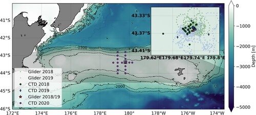
A 5-year research programme termed ROBES (‘Resilience of deep-sea benthic communities to the effects of sedimentation’) was developed to assess possible impacts from sedimentation caused by seabed disturbance (Clark et al. 2018; see https://niwa.co.nz/oceans/research-projects/resilience-of-deep-sea-benthic-fauna-to-sedimentation-from-seabed-mining). As part of this research, an ocean glider was deployed in austral Autumn/Winter in 2018 and 2019 on the central Chatham Rise (Figure 1), collecting full-depth profiles of various biophysical variables. Ship-based conductivity-Temperature-Depth (CTD) profiles were also collected in 2018 and 2019 with additional CTD profiles along and across the rise in June 2020.

Figure 1. Bathymetry of the Chatham Rise (from the General Bathymetric Chart of the Ocean (GEBCO)) showing the locations of the 2020 CTD casts (purple circles) and the STFZ (shaded area). The inset (a zoom of the grey box marked on central Chatham Rise) shows the mean position of the two glider deployments (red star) and the 2018 (green circles) and 2019 (blue diamonds) CTD casts. The light green and blue dots in the inset show the glider trajectories for the 2018 and 2019 deployments, respectively.

CTD data

Conductivity-temperature-depth (CTD) profiles were obtained on three voyages on RV Tangaroa. CTDs during May 2018 (21 May–2 June 2018) and June 2019 (5–28 June 2019), centred on 179.73°E, 43.36°S, coincided with two ocean glider deployments (described below) in the same area (Figure 1). A total of 46 CTD casts, 34 in May 2018 and 12 in June 2019, were collected at this location on the crest of the Chatham Rise. An additional 19 CTD casts were collected in June 2020 (10–19 June 2020). Six of the 2020 CTD casts were located longitudinally along 43.4°S between 178.90°E and 180.2°E. A further six and seven casts were located latitudinally between 42.8°S and 44°S at 179.2°E and 179.8°E, respectively (Figure 1). All hydrographic profiles were full water column (depth of c. 450 m) profiles and the data at each station were averaged into 2 decibar (m) bins.

Ocean glider surveys

Ocean gliders are a cost-effective, robust tool to collect high-resolution ocean data in a range of environments including shelf seas (e.g. Schaeffer et al. 2014; Ross et al. 2017) and polar regions (e.g. Schofield et al. 2013; Swart et al. 2015). These 1.5 m buoyancy-controlled, self-propelled autonomous underwater vehicles collect physical and bio-optical measurements of the water column (Schofield et al. 2007). Ocean gliders typically have horizontal speeds of 0.2–0.3 m/s and ascent/decent rates of 0.15–0.2 m/s and profile the water column in a sawtooth pattern.

The Teledyne Webb Research Slocum G2 glider deployed on Chatham Rise was equipped with a Seabird CTD sensor, a Wet Labs Environmental Characterization Optics sensor package (ECO puck), which measured chlorophyll-a (Chl-a) fluorescence, chromophoric dissolved organic matter (CDOM) and optical backscatter at 470, 532, 660, and 700 nm. In addition, the gilder was fitted with a Biospherical QSP sensor and an Aanderaa Oxygen Optode for measuring photosynthetically active radiation (PAR) and dissolved oxygen (DO) concentrations, respectively.

Two glider missions were carried out in approximately the same location on Chatham Rise (Figure 1) roughly one year apart. The first mission took place between 20 May 2018 and 2 June 2018 and collected 480 vertical profiles in the central part of Chatham Rise on the northern slopes centred on 179.73°E, 43.37°S (Figure 1). The second mission took place in roughly the same location as the first (centred on 179.74°E, 43.35°S) and collected 381 vertical profiles between 12 June 2019 and 25 June 2019 (Figure 1). During both deployments, the glider profiled from the sea surface to about 450 m water depth, typically to within 10 m of the seafloor.

Ancillary data

This study uses several additional independent datasets to investigate the oceanographic response on Chatham Rise to wind and buoyancy forcing. In particular, an atmospheric reanalysis product is used to determine the impact of wind and buoyancy forcing on the mixed layer while a high-resolution sea surface temperature data set is used to infer the distinction of and separation between STW and SAW (and thus the location of the STF).

Atmospheric data

Surface wind, evaporation, precipitation, shortwave and longwave radiative fluxes as well as latent and sensible heat were obtained from 6-hourly data sourced from the Japanese 55-year Reanalysis product (JRA-55; Kobayashi et al. 2015) produced by the Japanese Meteorological Agency (JMA). JRA-55 has a horizontal resolution of c. 55 km and was obtained for the periods commensurate with the observational data (i.e. 21 May–2 June 2018, 5–28 June 2019, 10–19 June 2020). The surface freshwater flux was calculated from evaporation (E) and precipitation (P) rates. The net surface heat flux (Q_net) was derived from net shortwave (Q_SW) and net longwave (Q_LW) radiative fluxes as well as latent (Q_lat) and sensible (Q_sen) heat fluxes: $Q_{net}=Q_{SW}+Q_{LW}+Q_{lat}+Q_{sen}$where Q_SW is the difference between incoming and outgoing shortwave radiation and Q_LW is the difference between incoming and outgoing longwave radiation. The sign convention used here is that a positive (negative) flux tends to warm (cool) the ocean surface.

The surface buoyancy flux (B_net) was calculated from the surface heat flux (Q_net) and the surface freshwater flux: $B_{net}=B_t+B_s$where B_t is the buoyancy flux attributable to surface heat flux, $B_t={\displaystyle \frac{g\alpha Q_{net}}{{\rho }_0{C}_p}}$and B_s is the contribution to the surface buoyancy flux due to the freshwater gain and loss due to precipitation and evaporation, $B_s=g\beta (E-P)So$where g is the gravitational acceleration (9.81 m/s²), α is the thermal expansion coefficient, ${\rho }_0$ is the average seawater density (1024.5 kg/m³), $C_p$ is the specific heat of seawater (4000 J/kg K), β is the haline contraction coefficient, and $So$ is a reference surface salinity (34.8 g/kg).

Sea surface temperature data

The Multi-scale Ultra-high Resolution (MUR) sea surface temperature (SST) data set produced by the Group for High Resolution Sea Surface Temperature (GHRSST) was used to complement the glider and CTD data. This data set, made available by the Jet Propulsion Laboratory (JPL) Physical Oceanography Distributed Active Archive Centre (DAAC; https://podaac.jpl.nasa.gov), provides high-resolution (0.01 × 0.01°), daily SST estimates. The level 4 data product of the current version (Version 4.1; https://doi.org/10.5067/GHGMR-4FJ04) combines the 1 km resolution MODIS SST observations with AVHRR, microwave and in-situ SST through a Multi-Resolution Variational Analysis (MRVA) method to produce gap-free gridded SST (Chin et al. 2017).

Several criteria have been used to identify the location of the STF around Aotearoa New Zealand. For example, Tilburg et al. (2002) used the 11–13°C surface isotherms to define the location of the STF east of New Zealand, with the upper (lower) bound isotherm indicative of the northern (southern) boundary of the STFZ. Behrens et al. (2021), on the other hand, used the 11°C isotherm and 34.8 isohaline between 100 and 500 m to identify the STF around New Zealand. In lieu of full water column, in-situ temperature and salinity measurements extending meridionally across the Chatham Rise for the periods of interest here, the 12°C isotherm from the SST data is used as proxy for the STF. This isotherm coincides with the maximum meridional SST gradient over Chatham Rise (Figure 7) and is therefore deemed a good proxy for the STF.

Boundary layers and stratification

A number of different criteria exists for characterising the mixed layer (ML) depths including gradient-based and property difference-based criteria (Dong et al. 2008). For the purposes of this study, a difference-based criterion is used to determine the depth of the ML. This method defines the ML depth as the depth where the oceanic property has changed from a near-surface reference value by a certain amount (e.g. de Boyer Montégut et al. 2004) and has also been used by others (e.g. Hadfield et al. 2007; Chiswell 2011; Chiswell et al. 2013) to determine the depth of the mixed layer in the southwest Pacific east of Aotearoa New Zealand and on Chatham Rise.

Here the ML depth is defined as the depth where the density difference exceeds 0.03 kg/m³ in reference to the density at 10 m depth ($\mathrm{\Delta }{\rho }_{10m}$ = 0.03 kg/m³) following the method of de Boyer Montégut et al. (2004). In addition to the ML depth, we also calculate the depth of the seasonal thermocline using the commonly used threshold of 0.125 kg/m³ (de Boyer Montégut et al. 2004; Chiswell 2011).

The density difference threshold method used to calculate the depth of the surface ML can also be used to determine the thickness of the bottom ML (e.g. Schaeffer et al. 2014; Todd 2017). Here the bottom ML thickness is defined as the depth where the density difference exceeds 0.04 kg/m³ in reference to the density at the bottom of each profile.

Stratification regulates vertical mixing which in turn is important for redistributing heat and nutrients. Furthermore, the intensity of stratification modulates primary production by controlling the amount of exposure of phytoplankton to light and nutrient conditions. The Brunt-Väisälä frequency (or buoyancy frequency; BVF), $N^2={\displaystyle \frac{-g}{{\rho }_0}{\displaystyle \frac{\mathrm{\partial }p}{\mathrm{\partial }z}}}$was calculated as a measure of the strength of stratification. Here, 9.81 m/s² is the acceleration due to gravity (g), ${\displaystyle \frac{\mathrm{\partial }p}{\mathrm{\partial }z}}$ is the vertical potential density gradient with water depth (z) (m), ${\rho }_0$ is the reference density (1027 kg/m³) and p is the potential density of seawater (kg/m³).

Results

Water mass properties

Temperature-salinity diagrams constructed from the two glider deployments and the CTD profile data show the presence of typical Southwest Pacific Ocean surface water masses, identified based on the description of Chatham Rise water masses provided by Sutton (2001). The two main water masses are Subtropical Water (STW) with temperatures of 12–15°C and salinity >34.8 g/kg and Subantarctic Water (SAW; Figure 2) with temperatures <12°C and salinity <34.6 g/kg. The latter dominated the upper 100 m in 2019 while the former dominated in 2018. The upper 100 m sampled in 2020 was characterised by both STW and SAW; however, the SAW was warmer and more saline (Figure 2) than the previous years, suggesting that it had mixed with STW.

Figure 2. Temperature-Salinity diagrams for (a) 2018 CTD casts, (b) 2019 CTD casts, (c) 2020 CTD casts and the 2018 (d) and 2019 (e) glider deployments. Colour indicates depth of the water column measurements. All data deeper than 350 m are plotted in black. Primary water masses sampled are indicated (STW = Subtropical Water; SAW = Subantarctic Water).

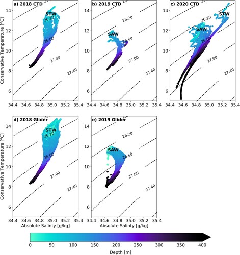
In 2018, warm (12–14.8°C), saline (34.8–35.1 g/kg) STW occupied the upper 100 m of the sampling location (Figure 2a and d). A subsurface central water mass with a characteristic linear T-S relationship and a wide range of temperatures (8–12.8°C) and salinities (34.6–34.9 g/kg) dominated the rest of the water column. STW was not present at the sampling location during 2019. Instead, a central water mass, occurring between 100–400 m, was overlaid by cold (11–12°C), fresh (34.6–34.9 g/kg) SAW (Figure 2b,e).

Unlike the 2018 and 2019 CTD casts, which sampled the same location, the CTD casts collected during 2020 sampled longitudinally and latitudinally across the central Chatham Rise (Figure 1). These casts separate out into two groups according to the sampling latitude. The four stations north of the 500 m isobath, were dominated by STW (>12°C, > 35 g/kg) in the upper 100 m overlying a subsurface central water mass (Figure 2c). At the rest of the 2020 stations, SAW (10–13°C, 34.6–35 g/kg) occurred in the top 100 m. The central water mass encountered at the northern most stations was slightly more saline than that observed at the other stations. In addition, the SAW sampled during 2020 was warmer and more saline compared to that sampled during 2019, suggesting mixing of this water mass with warmer, more saline STW.

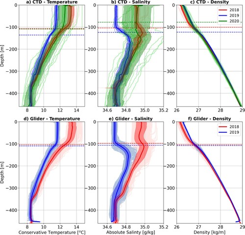
Vertical profiles of temperature, salinity and density from the glider deployments and CTD casts indicate that the surface ML on Chatham Rise was 80-140 m deep (Figure 3). The density profiles suggest that temperature is the main driver of stratification on Chatham Rise. Salinity-depth profiles from the glider missions as well as the CTD data indicate that there was a salinity maximum below the ML. In 2018 and 2020, the salinity maximum was located at about 150 m; however in 2019 the salinity maximum was shallower, located at c. 100–130 m.

Figure 3. Depth profiles of temperature (°C) (a, d), salinity (g/kg) (b, e) and density (kg/m³) (c, f) for the CTD data (2018 – red, 2019 – blue, 2020 – green) and the two glider deployments (2018 – red, 2019 – blue). Thick coloured lines indicate the mean temperature and salinity while the shading indicates the standard deviation. The coloured dashed lines indicate the mean depth of the mixed layer (ML).

Upper-ocean structure and variability

Physical structure

Ocean glider surveys provided high spatio-temporal resolution of the water column vertical structure over Chatham Rise. Figure 4 shows temperature, salinity, oxygen concentration and the squared Brunt-Väisälä frequency (BVF) from the two glider surveys. The Chatham Rise was delineated into three layers as distinguished by their thermal and haline characteristics. The relatively uniform upper- and near-bed layers are the surface and bottom ML, with a stable intermediate layer in between.

Figure 4. (a, b) Temperature (°C), (c, d) Salinity (g/kg), (e, f) oxygen concentration (μmol/l) and the squared Brunt-Väisälä frequency (s⁻¹) versus time and depth sampled by the ocean glider in May 2018 (left panels) and June 2019 (right panels). The cyan, white and purple lines indicate the mixed layer (ML) depth, depth of the seasonal thermocline and the top of the bottom ML respectively.

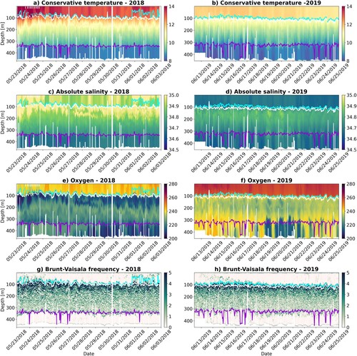
The upper ocean physical structure during the first glider deployment (May 2018) was characterised by a weakly stratified surface ML, comprising warm, saline STW (Figure 4). The depth of the ML ranged from 25 m to 123 m (mean = 79.3 ± 19.7 m). Higher temperature and salinity values at the beginning of the 2018 glider deployment corresponded to a shallower surface ML (30–100 m; mean = 70.4 ± 15.4 m). This was followed by a deepening of the ML (50–123 m; mean = 80.7 ± 13.2 m) due to decreased temperature and salinity that persisted for the majority of the deployment period (Figure 4a and c). Towards the end of the deployment period, increased temperature and salinity values resulted in a shallowing of the surface ML (25–106 m; mean = 63.2 ± 23.6 m). A distinct subsurface salinity maximum was observed in the well-stratified intermediate layer below the ML at depths of 100–200 m (Figure 4c). This subsurface salinity maximum was characterised by low oxygen concentrations (<220 µmol/l) (Figure 4e), whereas the overlying STW was well oxygenated (>240 µmol/l). The bottom c. 100 m of the water column was characterised by nearly homogenous temperatures (8–9°C) and salinities (34.6–34.8 g/kg) and low but variable oxygen concentrations (200–240 µmol/l). On average, this bottom ML was 97.6 ± 14.9 m thick but thinned to 30–40 m on multiple occasions.

During the second glider deployment (June 2019), the surface ML, comprising cold, fresh SAW, was deeper (mean = 98.3 ± 11.2 m), ranging from 53 to 131 m, and less variable compared to the 2018 ML (Figure 4). A shallower ML (53–107 m; mean = 89.8 ± 9.1 m) during the first half of the 2019 glider deployment was followed by a deepening of the ML (82–131 m; mean  = 103.6 ± 8.9 m) that persisted for the rest of the deployment period. The shallower surface ML corresponded to slightly higher temperature and salinity values in the upper 100 m, whereas the deeper ML was associated with a decrease in temperature and salinity (Figure 4b and d). The top 100 m displayed relatively homogenous temperatures and salinities in the vertical and with time, which is indicative of a well-mixed surface layer (Figure 4b and d). Oxygen concentrations measured during the second deployment were higher (210–260 µmol/l) throughout the water column (Figure 4f) in comparison to the concentrations measured in 2018 (210–250 µmol/l; Figure 4e). The upper 100 m was well oxygenated (>250 µmol/l) compared to the rest of the water column. A recurring oxygen minimum (<220 µmol/l) was recorded in the bottom c. 100–150 m of the water column between 17 and 22 June 2019 (Figure 4f). This oxygen minimum, characterised by slightly more saline water compared to the rest of the deployment period extended above the bottom ML, which had an average thickness of 113.6 m ± 25.0 m. (Figure 4d and e).

The time-depth sections of BVF from the glider deployments show that the highly variable surface ML observed during 2018 was synonymous with a weakly stratified upper layer (BVF ∼ 0) that extended to the seasonal thermocline found at 70–120 m-depth (Figure 4g). The seasonal thermocline corresponds to the depth of maximum water column buoyancy frequency. Trails of elevated stratification in the upper 100 m corresponded with shoaling of the ML (Figure 4g). The seasonal thermocline occurred at a similar depth range as the surface ML for the majority of the sampling period. However, during the last three days the seasonal thermocline was separated from the ML coinciding with the shoaling of the ML.

The deeper surface ML observed during 2019 coincided with a deeper seasonal thermocline located at 90–140 m and thus also a thicker weakly stratified upper layer (Figure 4h). The seasonal thermocline remained mostly separated from the ML for the duration of the sampling period. Both glider deployments showed a more stratified intermediate layer sandwiched between a weakly stratified surface and bottom layer. The intermediate layer sampled during the 2018 deployment was more stratified compared to 2019.

Spatial variability of mixed layer depth

Apart from the temporal variation in the surface ML depth observed in the glider data, the CTD casts collected in 2020 indicate that the ML over Chatham Rise also varies spatially (Figure 5). The CTD stations sampled longitudinally along 43.4°S (Figure 5a) in 2020 indicate that the ML, comprising a mixture of STW and SAW, was shallower at the two westernmost stations (178.9°E and 179.2°E) and the easternmost station (180.2°E) compared to the ML closer to the glider deployment location (179.5°E, 179.7°E, 180°E). The ML deepened from c. 90–100 m in the west to about 120 m before shallowing again to c. 100 m east of 180°E. The upper 100 m along this section was well oxygenated compared to the rest of the water column; however, elevated oxygen concentrations were observed in the bottom 100 m at the four central stations.

Figure 5. Depth profiles of temperature (°C) for the 2020 CTD stations collected longitudinally along 43.4°S (a) and latitudinally along 179.2°E (b) and 179.8°E (c). The colour of the temperature profiles indicate oxygen (µmol/l). The dashed red lines indicate the depth of the mixed layer. The second northern most station along 179.2° E was excluded due to erroneous data.

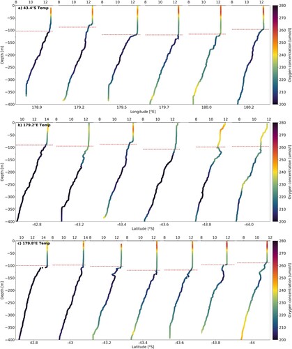
The CTD stations sampled latitudinally along 179.2°E (Figure 5b) and 179.8°E in 2020 (Figure 5c) indicate that the surface ML was shallower on the northern and southern flanks of Chatham Rise compared to a deeper ML on the crest (at 500 m depth) of the rise. The ML over the northern and southern flank of Chatham Rise was 90–100 m deep and was dominated by STW and SAW, respectively. On the crest of Chatham Rise, however, the ML was 110–120 m deep and comprised a mixture of STW and SAW. The ML over both flanks of the rise was well oxygenated compared to the rest of the water column with higher oxygen concentrations in the ML over the southern flank compared to the northern flank.

Biological structure

The vertical structure of Chl-a fluorescence on Chatham Rise was tightly coupled to that of the hydrographic structure (Figure 6a and b) with the depth of the maximum vertical gradient in Chl-a closely correlated with the ML depth (Figure 6c and d). Hence, phytoplankton were well mixed throughout the surface ML during both glider deployments. Elevated Chl-a concentrations were also confined to the ML during the 2020 CTD sampling period with the highest concentrations occurring at the stations sampled latitudinally along 179.8°E (Figure S2).

Figure 6. Glider chlorophyll a (Chl-a) concentration (mg/m3) (a and b) and vertical Chl-a gradient (dChl/dz) (c and d) for the May 2018 (left panels) and June 2019 (right panels) glider deployments. The cyan and white lines indicate the mixed layer (ML) depth and depth of the seasonal thermocline. (e and f) Depth averaged Chl-a concentrations from the glider deployments within the ML (black) and above the seasonal thermocline (red).

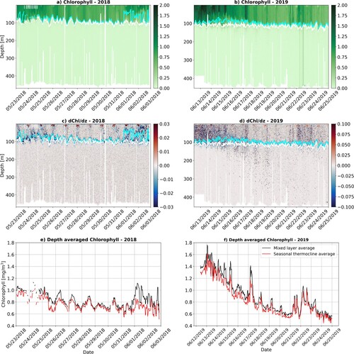
At the beginning of the 2018 sampling period, the depth averaged Chl-a concentration above the seasonal thermocline and within the ML was high (Figure 6a and e) but decreased steadily over a 9-day period. This decrease was followed by an abrupt increase in the averaged Chl-a within the ML in response to the shallowing of the ML. The average Chl-a within the ML and above the seasonal thermocline diverged during this period, reflecting a decoupling between the ML and the seasonal thermocline.

The depth-averaged Chl-a concentration within the ML and above the seasonal thermocline was markedly higher in 2019 compared to 2018 (Figure 6b) but a steady decrease over a 9-day period (Figure 6f) brought it down to similar levels observed in 2018. This decrease coincided with an increase in the ML depth and seasonal thermocline.

Discussion

Mechanisms of water mass variability over Chatham Rise

Warm, saline, low oxygen STW dominated the top 100 m over Chatham Rise in 2018, whereas cooler, fresher, high oxygen SAW dominated in 2019 (Figures 2 and 4). In 2020, SAW dominated in the top 100 m at the majority of the stations; however, it was warmer and more saline than the 2019 SAW suggesting that it had mixed with warmer, more saline STW. STW was also sampled in 2020 but was confined to the stations on the northern flank of Chatham Rise. Historical CTD measurements collected on Chatham Rise (collected in 1993–2012) show that STW, SAW and a mixture of both surface water masses is common over Chatham Rise, with the STW generally occurring on the northern flank of the rise (north of 42.8°S), SAW occurring on the southern flank (south of 43.2°S) and the mixed SAW-STW occurring over the central Chatham Rise (Figure S1). The STW sampled in 2020 had properties close to the STW (T ∼ 16°C, S ∼ 35.3 g/kg) found north of the rise (at 41°S; Chiswell and Sutton 1998), while the STW sampled in 2018 was slightly cooler and fresher (T ∼13°C, S ∼ 35 g/kg). The SAW sampled over Chatham Rise was slightly warmer and more saline (T ∼ 11.8° C, S ∼ 34.7 g/kg) than SAW (T ∼ 11°C, S ∼ 34.3 g/kg) found south of the rise (at 46°S; Chiswell and Sutton 1998).

The main causal mechanism of the observed surface water mass variability is the STF, in particular the geographic location of the front. The latitudinal position of the 12°C isotherm, used as a proxy for the location of the STF, shows that the STF was located south of the sampling location (at c. 43.8°S) in 2018 and 2020 whereas, in 2019 it was located just north of the sampling location (at c. 43.1 °S; Figure 7). The more southern (or northern) location of the STF facilitated the lateral advection of STW (or SAW) onto Chatham Rise.

Figure 7. Mean wind speed (m/s) (left panel) and meridional sea-surface temperature (SST) gradient (°C/km) (right panel) for the three sampling periods: (a, b) May 2018 (20 May–3 June 2018), (d, e) June 2019 (13–20 June 2019) and (g, h) June 2020 (9–20 June 2020). Black and blue vectors on the wind speed panels denote wind direction and Ekman transport, respectively. Black contours on the SST panels denote surface isotherms every 1°C with the bold contour highlighting the 12°C isotherm.

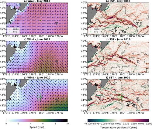
Behrens and Bostock (2023) showed that the location of the STF in the southwest Pacific is determined by the strength of the westerlies. Stronger westerly winds induce a northward migration of the STF due to enhanced northward Ekman transport. Weaker westerlies, on the other hand, result in a southward migration of the STF. Weak (<5 m/s) southwesterlies dominated over Chatham Rise during 2018 (Figure 7a) which resulted in weak northeastward Ekman transport and consequently the observed southward migration of the STF. Conversely, stronger (5 m/s) southwesterlies accompanied by strong northward Ekman transport in 2019 resulted in a northward shift of the STF (Figure 7c,d). As a result, SAW, characterised by SST values <12°C, was observed on the crest of the rise. Similar to 2018, weak northwesterly winds dominated over the rise which resulted in a southward migration of the STF (Figure 7e,f).

Mechanisms of mixed layer variability

Upper ocean stratification, and thus the depth of the ML, is modulated by wind induced vertical mixing and air–sea buoyancy fluxes (Fauchereau et al. 2011; Taylor and Ferrari 2011). Increased wind stress enhances mechanical mixing which acts to deepen the ML. Buoyancy loss, on the other hand, increases stratification which, in turn, inhibits vertical mixing which can result in a shallower ML.

The shallow surface ML (c. 80 m) in 2018 compared to 2019 was a result of decreased mechanical mixing due to overall weaker southerly winds (Figure 8) combined with a negative surface buoyancy flux due to heat loss to the atmosphere (Figure 9). The buoyancy gain acted to increase the stratification by stabilising the water column which further impeded vertical mixing. Towards the end of the 2018 sampling period, a relaxation of the southerly winds resulted in heat gain and positive buoyancy flux. The weaker mechanical mixing countered the effects of the buoyancy loss (reduced stratification leading to deeper mixed layer) resulting in restratification and a shoaling of the ML.

Figure 8. Time evolution of meridional Ekman transport and wind velocity during the (a) 2018 glider deployment, (b) 2019 glider deployment and (c) 2020 CTD hydrographic survey as derived from the JRA55 reanalysis.

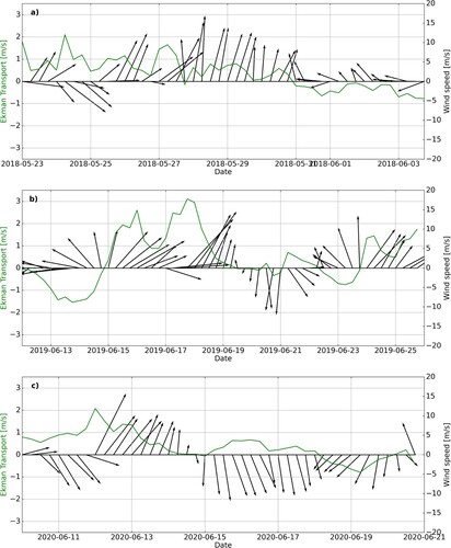
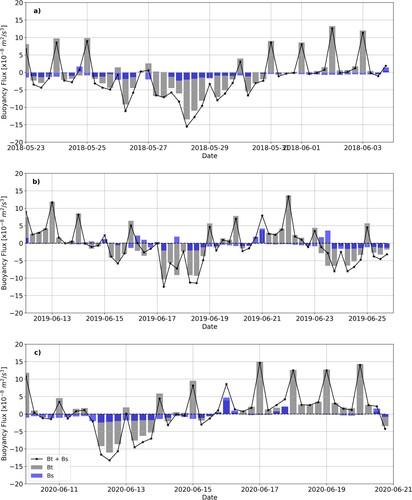
Figure 9. Time evolution of surface buoyancy flux (×10⁻⁸ m²/s³) due to heat flux (Bt, grey bars) and freshwater flux (Bs, blue bars) for the (a) May 2018, (b) June 2019 and (c) June 2020 sampling periods as derived from the JRA55 reanalysis. The black line shows the total buoyancy flux (Bt + Bs).

The deeper (c. 100 m) more stable surface ML observed in 2019 (Figure 5) was the result of stronger, less variable winds (Figure 8) and a predominantly positive surface buoyancy flux (Figure 9). Strong negative buoyancy flux due to strong negative heat flux dominated at the start of the 2019 sampling period (not shown). This would have resulted in a shallower ML due to increased stratification and reduced vertical mixing. However, the effects of the negative buoyancy flux were countered by strong southwesterly winds that set-up a ML of intermediate depth which was sustained during the first few days of the 2019 sampling period. The predominantly strong southerly winds during the rest of the 2019 sampling period acted to deepen the ML despite periods of alternating buoyancy forcing.

Biological response to mixed layer variability

The overall lower Chl-a concentrations observed over Chatham Rise in 2018 can be attributed to the dominance of macronutrient-poor STW in the surface ML. In general, we infer that Chl-a concentrations decreased over the 2018 sampling period because of nutrient depletion. However, elevated Chl-a concentrations toward the end of the sampling period coincided with restratification of the ML induced by the relaxation of southerly winds. The shallower mixed layer would have allowed phytoplankton to exploit higher irradiance intensities near the surface while the weaker vertical mixing would have reduced the flux of phytoplankton out of the euphotic zone. Both of these mechanisms likely contributed to the elevated Chl-a concentrations toward the end of the 2018 sampling period. The weaker vertical mixing, however, also suggests reduced input of nutrients from below the ML, and thus the bloom was short-lived as nutrient consumption is outpaced by nutrient supply (Chiswell et al. 2013; 2015).

Surprisingly, Chl-a concentrations in 2019, when HNLC SAW dominated the surface ML, where higher compared to 2018. The initial elevated Chl-a concentrations observed in 2019 can be attributed to elevated Chl-a concentrations during the preceding month. The sustained elevated Chl-a concentrations are likely a result of nutrient injection from below the ML because of increased vertical mixing due to stronger southwesterlies. Similar to 2018, Chl-a concentrations show a decreasing trend likely due to nutrient depletion. The deepening of the ML also contributed to the reduction in Chl-a concentrations as a deeper ML mixes phytoplankton deeper in the water column and reduces phytoplankton light availability (e.g. Boyd et al. 1999).

Implications for resource management and human activities

Variability in major oceanographic features such as the STF is clearly important for interpreting and understanding the likely impact of human activities such as bottom trawling or seabed mining. The effects of shifting currents and water masses on the distribution of productivity, prey organisms, and the sinking of particulate organic matter need to be considered for benthic communities, as well as for fisheries. On the Chatham Rise, such factors are likely important for their links with the hoki fishery (e.g. McClatchie et al. 1997, 2005). In relation to seabed mining, the International Seabed Authority regulates exploration for deep-sea minerals on the seafloor beyond national jurisdiction. In its recommendations for the acquisition of baseline environmental data by contractors (International Seabed Authority 2020), it is stressed that data need to be collected with sufficient temporal resolution to adequately characterise the oceanographic environment, potentially over at least three years. The variability shown in this study highlights the importance of such a time series to describe how changes in both pelagic and benthic communities might be related to variability in physical oceanographic characteristics and patterns.

Conclusions

The present study uses high-resolution ocean glider and CTD data from Chatham Rise over three consecutive years (2018–2020) to examine the variability of surface water masses, the mixed layer and phytoplankton biomass accumulation on Chatham Rise. In addition, an atmospheric reanalysis product is used to determine the causal mechanisms behind the water mass, STF and mixed layer variability.

The water column of the STFZ over Chatham Rise consists of a well-defined three-layer structure comprised of a stable intermediate layer sandwiched between a well-mixed surface and bottom layer. The in-situ data showed that different water masses can dominate the surface mixed layer at different times. This variability in surface water masses appears to be related to the position of the STF which is modulated by wind forcing.

The ML over Chatham Rise exhibited considerable temporal and spatial variability and a strong relationship was observed between surface chlorophyll concentrations and the ML depth. Wind driven vertical mixing appears to be the main causal mechanism of the ML variability observed over Chatham Rise with surface buoyancy flux only playing a small role.

Oceanic variability, including the location of the STF, and changes in patterns of planktonic productivity, have implications for the distribution of biological communities and fisheries, as well as understanding natural variability. Knowledge of such variability in environmental baseline data is required for predicting or measuring the impacts of human activities such as bottom trawling and potential seabed mining and informing spatial and resource management decisions and strategies.

Acknowledgements

The authors would like to acknowledge funding from the Ministry of Business, Innovation and Employment Endeavour Fund (contract CO1X1614). Thanks to the scientific crew on the three ROBES voyages, especially the NIWA CTD operators, Sarah Searson, Olivia Price, Will Quinn and Steve George and the glider operators, Fiona Elliot and Khushboo Jhurgoo. Thanks also to Matt Walkington (NIWA) for setting up the CTD and processing the CTD data. The authors would also like to thank the officers and crew of the RV Tangaroa. We thank the two journal reviewers, whose careful comments improved the manuscript.

Disclosure statement

No potential conflict of interest was reported by the author(s).

Additional information

Funding

This work was supported by the Ministry of Business, Innovation and Employment [grant number CO1X1614].

References

- Behrens E, Bostock H. 2023. The response of the Subtropical Front to changes in the Southern Hemisphere westerly winds – evidence from models and observations. Journal of Geophysical Research: Oceans. 128:e2022JC019139.
- Behrens E, Hogg AM, England MH, Bostock H. 2021. Seasonal and interannual variability of the subtropical front in the New Zealand region. Journal of Geophysical Research: Oceans. 126(2):e2020JC016412.
- Belkin IM. 1988. Main hydrological features of the central South Pacific. In: Vinogradov ME, Flint MV, editors. Ecosystems of the subantarctic zone of the Pacific Ocean. Moscow: Nauka; p. 21–28. Russian.
- Belkin IM, Gordon AL. 1996. Southern Ocean fronts from the Greenwich meridian to Tasmania. Journal of Geophysical Research: Oceans. 101(C2):3675–3696.
- Boyd P, LaRoche J, Gall M, Frew R, McKay RML. 1999. Role of iron, light, and silicate in controlling algal biomass in subantarctic waters SE of New Zealand. Journal of Geophysical Research: Oceans. 104(C6):13395–13408.
- Boyd PW, McTainsh G, Sherlock V, Richardson K, Nichol S, Ellwood M, Frew R. 2004. Episodic enhancement of phytoplankton stocks in New Zealand subantarctic waters: contribution of atmospheric and oceanic iron supply. Global Biogeochemical Cycles. 18:GB1029.
- Bradford-Grieve JM, Boyd PW, Chang FH, Chiswell S, Hadfield M, Hall JA, James MR, Nodder SD, Shushkina EA. 1999. Pelagic ecosystem structure and functioning in the Subtropical Front region east of New Zealand in austral winter and spring 1993. Journal of Plankton Research. 21(3):405–428.
- Bradford-Grieve JM, Chang FH, Gall M, Pickmere S, Richards F. 1997. Size-fractionated phytoplankton standing stocks and primary production during austral winter and spring 1993 in the Subtropical Convergence region near New Zealand. New Zealand Journal of Marine and Freshwater Research. 31(2):201–224.
- Burls NJ, Reason CJC. 2006. Sea surface temperature fronts in the midlatitude South Atlantic revealed by using microwave satellite data. Journal of Geophysical Research: Oceans. 111(C8):C08001.
- Chatham Rock Phosphate. 2022. [Accessed 2022 October 12]. https://www.rockphosphate.co.nz/the-project.
- Chin TM, Vazquez-Cuervo J, Armstrong EM. 2017. A multi-scale high-resolution analysis of global sea surface temperature. Remote Sensing of Environment. 200:154–169.
- Chiswell SM. 1994. Acoustic Doppler current profiler measurements over the Chatham Rise. New Zealand Journal of Marine and Freshwater Research. 28(2):167–178.
- Chiswell SM. 2001. Eddy energetics in the subtropical front over the Chatham Rise, New Zealand. New Zealand Journal of Marine and Freshwater Research. 35(1):1–15.
- Chiswell SM. 2011. Annual cycles and spring blooms in phytoplankton: don’t abandon Sverdrup completely. Marine Ecology Progress Series. 443:39–50.
- Chiswell SM, Bradford-Grieve J, Hadfield MG, Kennan SC. 2013. Climatology of surface chlorophyll a, autumn-winter and spring blooms in the southwest Pacific Ocean. Journal of Geophysical Research: Oceans. 118(2):1003–1018.
- Chiswell SM, Calil PHR, Boyd PW. 2015. Spring blooms and annual cycles of phytoplankton: a unified perspective. Journal of Plankton Research. 37(3):500–508.
- Chiswell SM, Safi KA, Sander SG, Strzepek R, Ellwood MJ, Milne A, Boyd PW. 2019. Exploring mechanisms for spring bloom evolution: contrasting 2008 and 2012 blooms in the southwest Pacific Ocean. Journal of Plankton Research. 41(3):329–348.
- Chiswell SM, Sutton PJ. 1998. A deep eddy in the antarctic intermediate water north of the Chatham Rise. Journal of Physical Oceanography. 28(3):535–540.
- Clark MR, Nodder S, O’Callaghan J, Rowden AA, Cummings V, Hickey C. 2018. Effects of sedimentation from deep-sea mining: a benthic disturbance experiment off New Zealand. Deep-Sea Life. 12:18–19.
- Deacon GER. 1982. Physical and biological zonation in the Southern Ocean. Deep Sea Research Part A. Oceanographic Research Papers. 29(1):1–15.
- de Boyer Montégut C, Madec G, Fischer AS, Lazar A, Iudicone D. 2004. Mixed layer depth over the global ocean: an examination of profile data and a profile-based climatology. Journal of Geophysical Research: Oceans. 109(C12):C12003.
- Dong S, Sprintall J, Gille ST, Talley L. 2008. Southern Ocean mixed-layer depth from Argo float profiles. Journal of Geophysical Research: Oceans. 113(C6):C06013.
- Ellis JI, Clark MR, Rouse HL, Lamarche G. 2017. Environmental management frameworks for offshore mining: the New Zealand approach. Marine Policy. 84:178–192.
- Fauchereau N, Tagliabue A, Bopp L, Monteiro PMS. 2011. The response of phytoplankton biomass to transient mixing events in the Southern Ocean. Geophysical Research Letters. 38:L17601.
- Fisheries New Zealand. 2022. Fisheries assessment plenary, May 2022: stock assessments and stock status. Wellington: Compiled by the Fisheries Science Team. Fisheries New Zealand.
- Graham RM, Boer D,MA. 2013. The dynamical subtropical front. Journal of Geophysical Research: Oceans. 118(10):5676–5685.
- Hadfield MG, Rickard GJ, Uddstrom MJ. 2007. A hydrodynamic model of Chatham Rise, New Zealand. New Zealand Journal of Marine and Freshwater Research. 41(2):239–264.
- Heath RA. 1985. A review of the physical oceanography of the seas around New Zealand – 1982. New Zealand Journal of Marine and Freshwater Research. 19(1):79–124.
- International Seabed Authority. 2020. [Accessed 2022 October 12]. https://www.isa.org.jm/index.php/our-work/protection-marine-environment.
- Kobayashi S, Ota Y, Harada Y, Ebita A, Moriya M, Onoda H, Onogi K, Kamahori H, Kobayashi C, Endo H, Miyaoka K. 2015. The JRA-55 reanalysis: general specifications and basic characteristics. Journal of the Meteorological Society of Japan. Ser. II. 93(1):5–48.
- Kostianoy AG, Ginzburg AI, Frankignoulle M, Delille B. 2004. Fronts in the Southern Indian Ocean as inferred from satellite sea surface temperature data. Journal of Marine Systems. 45(1–2):55–73.
- Marra JF, Chamberlin WS, Knudson CA, Rhea WJ, Ho C. 2023. Parameters for the depth of the ocean’s productive layers. Frontiers in Marine Science. 10:536.
- McClatchie S, Millar RB, Webster F, Lester PJ, Hurst R, Bagley N. 1997. Demersal fish community diversity off New Zealand: is it related to depth, latitude and regional surface phytoplankton? Deep Sea Research Part I: Oceanographic Research Papers. 44(4):647–667.
- McClatchie S, Pinkerton M, Livingston NE. 2005. Relating the distribution of a semi-demersal fish, Macruronus novaezelandiae, to their pelagic food supply. Deep Sea Research Part I: Oceanographic Research Papers. 52(8):1489–1501.
- Murphy RJ, Pinkerton MH, Richardson KM, Bradford-Grieve JM, Boyd PW. 2001. Phytoplankton distributions around New Zealand derived from SeaWiFS remotely-sensed ocean colour data. New Zealand Journal of Marine and Freshwater Research. 35(2):343–362.
- Nodder SD, Boyd PW, Chiswell SM, Pinkerton MH, Bradford-Grieve JM, Grieg MJN. 2005. Temporal coupling between surface and deep ocean biogeochemical processes in contrasting subtropical and subantarctic water masses, southwest Pacific Ocean. Journal of Geophysical Research. 110:C12017.
- Nodder SD, Northcote LC. 2001. Episodic particulate fluxes at southern temperate mid-latitudes (42–45°S) in the Subtropical Front region, east of New Zealand. Deep Sea Research Part I: Oceanographic Research Papers. 48(3):833–864.
- Ross T, Craig SE, Comeau A, Davis R, Dever M, Beck M. 2017. Blooms and subsurface phytoplankton layers on the Scotian Shelf: insights from profiling gliders. Journal of Marine Systems. 172:118–127.
- Safi KA, Gutiérrez-Rodríguez A, Hall JA, Pinkerton MA. 2023. Phytoplankton dynamics, growth and microzooplankton grazing across the subtropical frontal zone, east of New Zealand. Deep Sea Research Part II: Topical Studies in Oceanography. 208:105271.
- Schaeffer A, Roughan M, Wood JE. 2014. Observed bottom boundary layer transport and uplift on the continental shelf adjacent to a western boundary current. Journal of Geophysical Research: Oceans. 119(8):4922–4939.
- Schofield O, Ducklow H, Bernard K, Doney S, Patterson-Fraser D, Gorman K, Martinson D, Meredith M, Saba G, Stammerjohn S, Steinberg D. 2013. Penguin biogeography along the West Antarctic Peninsula: testing the canyon hypothesis with Palmer LTER observations. Oceanography. 26(3):204–206.
- Schofield O, Kohut J, Aragon D, Creed L, Graver J, Haldeman C, Kerfoot J, Roarty H, Jones C, Webb D, Glenn S. 2007. Slocum gliders: robust and ready. Journal of Field Robotics. 24(6):473–485.
- Sutton P. 2001. Detailed structure of the subtropical front over Chatham Rise, east of New Zealand. Journal of Geophysical Research: Oceans. 106(C12):31045–31056.
- Sverdrup H. 1953. On conditions of the vernal blooming of phytoplankton. ICES Journal of Marine Science. 18(3):287–295.
- Swart S, Thomalla SJ, Monteiro PM. 2015. The seasonal cycle of mixed layer dynamics and phytoplankton biomass in the Sub-Antarctic Zone: a high-resolution glider experiment. Journal of Marine Systems. 147:103–115.
- Taylor AH, Harbour DS, Harris RP, Burkill PH, Edwards ES. 1993. Seasonal succession in the pelagic ecosystem of the North Atlantic and the utilization of nitrogen. Journal of Plankton Research. 15(8):875–891.
- Taylor JR, Ferrari R. 2011. Ocean fronts trigger high latitude phytoplankton blooms. Geophysical Research Letters. 38(23):L23601.
- Tilburg CE, Hurlburt HE, O'Brien JJ, Shriver JF. 2002. Remote topographic forcing of a baroclinic western boundary current: an explanation for the Southland Current and the pathway of the Subtropical Front east of New Zealand. Journal of Physical Oceanography. 32(11):3216–3232.
- Todd RE. 2017. High-frequency internal waves and thick bottom mixed layers observed by gliders in the Gulf Stream. Geophysical Research Letters. 44(12):6316–6325.
- Uddstrom MJ, Oien NA. 1999. On the use of high-resolution satellite data to describe the spatial and temporal variability of sea surface temperatures in the New Zealand region. Journal of Geophysical Research: Oceans. 104(C9):20729–20751.
- Zentara SJ, Kamykowski D. 1981. Geographic variation in the relationship between silicic acid and nitrate in the South Pacific Ocean. Deep Sea Research, Part A. 28:455–465.
- Zhou K, Nodder SD, Dai M, Hall JA. 2012. Insignificant enhancement of export flux in the highly productive Subtropical Front, east of New Zealand: a high-resolution study of particle export fluxes based on 234 Th:238 U disequilibria. Biogeosciences. 9(3):973–992.