Informing Performance Metrics of Advanced I&C Systems for Liquid Fueled Fast Molten Salt Reactors

Abstract

This work establishes a generic multiphysics tool for liquid-fueled molten salt reactors (LFMSRs) to select key installation locations and specify the expected operating temperature range for the development of advanced instrumentation and control systems, particularly distributed temperature sensors using fiber optics. A commercial computation fluid dynamics package (STAR-CCM+) is used to formulate a neutronics and thermal-hydraulic coupled solver, showing good agreement with a recent benchmark problem developed for evaluating the coupling methodology of neutronics and thermal hydraulics. The multiphysics model is then applied to the reference molten chloride salt fast reactor (MCFR) design under development by TerraPower based on publicly available information. The available two-dimensional axisymmetric model for the reactor core is used for coupling calculations, and system component details are leveraged using the lumped method to complete the energy balance. The dynamic responses of the MCFR model are investigated during operational transients, such as unprotected loss-of-flow and uniform perturbation scenarios. Maximum temperature and local temperature distributions are characterized during unprotected loss of flow and unprotected loss of heat sink events. The thermal responses of the fuel salt and core components are analyzed from induced perturbation of the system parameters, such as the flow rate and the heat sink capacity. The results motivate the use of continuous monitoring of the temperature variation in real time along the reflector region with the use of fiber optics to validate the multiphysics code to support a reactor’s licensing basis, as well as to support the structural longevity and improve safety in LFMSRs.

Keywords:

• Molten salt reactor
• liquid fuel
• multiphysics
• distributed fiber-optic sensing
• core temperature sensing

I. INTRODUCTION

Liquid-fueled molten salt reactors (LFMSRs) are a Generation IV reactor concept that has gained interest in the past few decades due to their intrinsic safety. LFMSRs were successfully demonstrated by the Aircraft Reactor Experiment and later the Molten Salt Reactor Experiment (MSRE) at Oak Ridge National Laboratory in the 1950s and 1960s. Presently, conceptual LFMSR designs are moving toward using a fast neutron spectrum because of its safety and economic advantages. The fast spectrum, enabled by chloride fuel salt, has advantages in breeding within the uranium and plutonium fuel cycle or in a plutonium and minor actinide burning scheme with the high solubility of actinides and harder neutron spectrum. The fast spectrum also allows the reactor to operate with high core power density, resulting in a reduction of the required volume of highly radioactive fueled salt. Research efforts have been made on the development of LFMSRs to be deployed in the near term, such as the molten chloride fast reactor (MCFR) designed by TerraPower in the United States¹ and the stable salt reactor designed by Moltex Energy in the United Kingdom and Canada.²

Nevertheless, no commercial LFMSR design concept has ever been demonstrated. The unique and complex physical phenomena exhibited by this type of reactor concept will likely lead to a lengthy research and development (R&D) pathway to support the licensing process in the absence of any detailed prior operational data. To accelerate the deployment of new reactor designs for commercial use, advanced instrumentation and control (I&C) techniques can be implemented to provide test reactor verification and to provide regulatory confidence through a high level of data visibility. One of the promising candidates for advanced I&C is using fiber-optic sensors, particularly distributed, single-crystal fiber temperature sensors that are under development as part of an ongoing Advanced Research Projects Agency-EnergyARPA-E grant led by the National Energy Technology Laboratory. Fiber optics can be used for temperature profiling at multiple sensing locations, as well as distributed strain or vibration sensing for mechanical diagnosis along the same length of optical fiber.^3,4 This feature enables the detection and location of hot spots, temperature variations, and mechanical loads in the core at the same time. Since LFMSR designs are characterized by complex flow patterns of internally heated molten-state fuel flowing in various core geometries, it is crucial to refine the key spatial locations and expected temperature range for fiber-optic sensor development. At this point, numerical simulation plays an essential role in developing advanced I&C to support the R&D pathway for LFMSRs.

The presence of strong and nonlinear coupling between neutronics and thermal hydraulics in LFMSRs makes this type of reactor modeling challenging. The liquid fuel flow transports delayed neutron precursors (DNPs), making their concentrations in the core dependent on the flow parameters. The impact of internal heat generation in liquid fuel and reactivity feedback from temperature and fuel density variations should be considered as well. A comprehensive overview of modeling efforts undertaken for LFMSRs are summarized in Ref. 5. Extending traditional codes or one-dimensional (1-D) simplifications and sets of correlations has shown promise in analyzing thermal spectrum molten salt reactors (MSRs), such as extending MSRE results to other reactors with segregated flow channels, similar to water-cooled reactors using fuel pins. However, currently proposed LFMSR cores consist of a singular flow channel, where complex fuel salt flow patterns can play an important role depending on the core geometry.^6–9 Therefore, it is vital to couple the thermal-hydraulic influences on neutronics fields using higher-fidelity tools.

The growth of computational power over time has allowed for the adoption of high-fidelity multiphysics computational fluid dynamics (CFD) approaches in lieu of the legacy 1-D approach for thermal-hydraulic assessment of the MSRE. Cammi et al.⁵ proposed a coupled neutronics and thermal-hydraulic model implemented in the same COMSOL simulation environment. They introduced a multigroup diffusion-based neutronics solver along with Reynolds-averaged Navier-Stokes (RANS) and energy equations for a thermal-hydraulic solver. Aufiero et al.¹⁰ developed a MSR multiphysics model within the OpenFOAM multiphysics toolkit. They implemented the neutron diffusion equation and transport equations for the flowing precursors along with a single-phase incompressible RANS model. Lindsay et al.¹¹ developed the open-source simulation tool for MSRs called Moltre. They constructed a deterministic neutronics and thermal-hydraulic solver in the multiphysics object-oriented simulation environment (MOOSE) framework. Most of research on recent multiphysics tools mentioned previously has been conducted to revisit the MSRE, to perform design studies of LFMSRs mainly using fluoride-based salt, to simulate particular phenomenon such as solid particle or inert gas transport,^12,13 or to extend existing software or codes developed for a MSR updating coupling scheme between neutronics and thermal hydraulics.^14–16 Transient simulations of LFMSRs using those multiphysics tools have been focused on the core domain only to assess whether such a design meets the safety criteria from maximum temperature of the fuel salt.^8,17

Recent LFMSR designs targeting near-term deployment adopt chloride-based salt because of its advantages in the economic utilization of the fissile materials¹⁸ and cost-effective fuel fabrication using techniques like pyroprocessing.⁸ Molten chloride salts are known to corrode metal alloys at elevated temperatures,¹⁹ and flow and thermal conditions must be evaluated for structural longevity calculations in commercial applications.²⁰ For I&C considerations, local temperatures and mechanical loads in core structures are of interest. Dynamic analysis of a MSR has been performed for the core region only for the simplicity of the modeling by setting the inlet temperature as a fixed input value.^21,22 In the present work, a more complete LFMSR model is provided using chloride salts and modeled core structures, including the reflector and the vessel walls. The model is implemented in a multiphysics tool taking into account the primary loop and the connected intermediate system components to provide performance metrics for distributed temperature sensors.

In this paper, we establish a generic MSR multiphysics CFD model for simulating LFMSRs by applying a commercially available CFD code (STAR-CCM+) (Ref. 23). A diffusion-based neutronics solver is implemented in passive scalar transport form for neutron flux and precursors. To evaluate the capability of the simulation tool, we compared benchmark results for fast spectrum MSRs (Ref. 24). Then we investigated the behavior of the LFMSR simulation for the conceptual TerraPower reference design¹ during operational transients. Based on these results, we recommend locations and necessary operating ranges for the installation of fiber-optic temperature sensors to best capture important transient thermal data to provide improved estimates of reactor material lifetimes and to enable quicker responses to abnormal operating conditions. The sensors’ operational range and thermal responses are estimated under typical incidental situations, such as pump and heat exchange failure and hypothetical events in which the flow velocity and temperature field are fluctuating. We hope that these additional levels of detail, which have been lacking attention in the literature thus far, can aid designers and engineers implementing these systems in the future.

II. MULTIPHYSICS MODEL OF A LFMSR

The neutronics model in this paper is based on one-group, time-dependent neutron diffusion theory. Flow effects on the neutron flux itself are minimal because the speed of neutron fission is orders of magnitude faster than the fuel flow rate.²⁵ Instead, DNPs have impacts on the neutron importance due to their movement and decay in the primary loop. To incorporate fluid flow effects, DNP balance equations are extended to include a convection term. The one-group neutron diffusion equation and six-group DNP balance equation are shown in Eqs. (1)(1) $\frac{1}{v}\frac{\mathrm{\partial }\varphi }{\mathrm{\partial }t}=\mathrm{\nabla }\cdot \left(D\mathrm{\nabla }\varphi \right)+\left(1-{\beta }_{tot}\right)\nu {\mathrm{\Sigma }}_f\varphi -{\mathrm{\Sigma }}_a\varphi +\sum _{i=1}^6{\lambda }_i{C}_i$(1) and (2)(2) $\frac{\mathrm{\partial }{C}_i}{\mathrm{\partial }t}+\mathrm{\nabla }\cdot \left(\vec{U}{C}_i\right)={\beta }_i\nu {\mathrm{\Sigma }}_f\varphi -{\lambda }_i{C}_i.$(2) :

(1) $\frac{1}{v}\frac{\mathrm{\partial }\varphi }{\mathrm{\partial }t}=\mathrm{\nabla }\cdot \left(D\mathrm{\nabla }\varphi \right)+\left(1-{\beta }_{tot}\right)\nu {\mathrm{\Sigma }}_f\varphi -{\mathrm{\Sigma }}_a\varphi +\sum _{i=1}^6{\lambda }_i{C}_i$(1)

and

(2) $\frac{\mathrm{\partial }{C}_i}{\mathrm{\partial }t}+\mathrm{\nabla }\cdot \left(\vec{U}{C}_i\right)={\beta }_i\nu {\mathrm{\Sigma }}_f\varphi -{\lambda }_i{C}_i.$(2)

The dependencies of the cross sections and diffusion coefficient on the fuel salt temperature and density are introduced as Eqs. (3)(3) $\mathrm{\Sigma }\left(T\right)=\frac{\rho \left(T\right)}{\rho \left(T_{ref}\right)}\left[\mathrm{\Sigma }\left(T_{ref}\right)+{\alpha }_{\mathrm{\Sigma }}log\frac{T}{T_{ref}}\right]$(3) and (4(4) $D\left(T\right)=\frac{\rho \left(T_{ref}\right)}{\rho \left(T\right)}\left[D\left(T_{ref}\right)+{\alpha }_{D}log\left(\frac{T}{T_{ref}}\right)\right].$(4) ), considering the Doppler effect and salt expansion feedback, where T_ref indicates the reference temperature, 900 K:

(3) $\mathrm{\Sigma }\left(T\right)=\frac{\rho \left(T\right)}{\rho \left(T_{ref}\right)}\left[\mathrm{\Sigma }\left(T_{ref}\right)+{\alpha }_{\mathrm{\Sigma }}log\frac{T}{T_{ref}}\right]$(3)

and

(4) $D\left(T\right)=\frac{\rho \left(T_{ref}\right)}{\rho \left(T\right)}\left[D\left(T_{ref}\right)+{\alpha }_{D}log\left(\frac{T}{T_{ref}}\right)\right].$(4)

The thermal-hydraulic MSR model is based on the Navier Stokes equation. The mass, momentum, and energy conservation equations are expressed as Eqs. (5)(5) $\frac{\mathrm{\partial }\rho }{\mathrm{\partial }t}+\mathrm{\nabla }\cdot \left(\rho \vec{U}\right)=0,$(5) , (6)(6) $\frac{\mathrm{\partial }\left(\rho \vec{U}\right)}{\mathrm{\partial }t}+\mathrm{\nabla }\cdot \left(\rho \vec{U}\otimes \vec{U}\right)=-\mathrm{\nabla }\cdot \left(pI\right)+\mathrm{\nabla }\cdot T,$(6) , and (7)(7) $\frac{\mathrm{\partial }\left(\rho E\right)}{\mathrm{\partial }t}+\mathrm{\nabla }\cdot \left(\rho E\vec{U}\right)=-\mathrm{\nabla }\cdot q+\mathrm{\nabla }\cdot \left(T\cdot \vec{U}\right)+S_E.$(7) , respectively²³:

(5) $\frac{\mathrm{\partial }\rho }{\mathrm{\partial }t}+\mathrm{\nabla }\cdot \left(\rho \vec{U}\right)=0,$(5)

(6) $\frac{\mathrm{\partial }\left(\rho \vec{U}\right)}{\mathrm{\partial }t}+\mathrm{\nabla }\cdot \left(\rho \vec{U}\otimes \vec{U}\right)=-\mathrm{\nabla }\cdot \left(pI\right)+\mathrm{\nabla }\cdot T,$(6)

and

(7) $\frac{\mathrm{\partial }\left(\rho E\right)}{\mathrm{\partial }t}+\mathrm{\nabla }\cdot \left(\rho E\vec{U}\right)=-\mathrm{\nabla }\cdot q+\mathrm{\nabla }\cdot \left(T\cdot \vec{U}\right)+S_E.$(7)

Precursors contributing to the decay heat are modeled separately in three groups, similar to DNPs, in Eq. (8)(8) $\frac{\mathrm{\partial }{D}_i}{\mathrm{\partial }t}+\mathrm{\nabla }\cdot \left(\vec{U}{D}_i\right)={\beta }_{d,i}{E}_f{\mathrm{\Sigma }}_f\varphi -{\lambda }_{d,i}{D}_i.$(8) :

(8) $\frac{\mathrm{\partial }{D}_i}{\mathrm{\partial }t}+\mathrm{\nabla }\cdot \left(\vec{U}{D}_i\right)={\beta }_{d,i}{E}_f{\mathrm{\Sigma }}_f\varphi -{\lambda }_{d,i}{D}_i.$(8)

Total heat generation is defined as the sum of the fission heat and decay heat, which is included in the energy balance equation as Eq. (9)(9) $Q=Q_{fission}+Q_{decay}=\left(1-{\beta }_{d,tot}\right)E_f{\mathrm{\Sigma }}_f\varphi +\sum _{i=1}^3{\lambda }_{d,i}{D}_i.$(9) :

(9) $Q=Q_{fission}+Q_{decay}=\left(1-{\beta }_{d,tot}\right)E_f{\mathrm{\Sigma }}_f\varphi +\sum _{i=1}^3{\lambda }_{d,i}{D}_i.$(9)

Outside the core region, primary loop components, such as the heat exchanger, hot leg, and cold leg, are considered as zero-dimensional models. The thermal-hydraulic model is based on the simple energy balance for each component, considering no heat loss in the hot leg and cold leg, and a single term for heat removal via the heat exchanger in the coolant loop as Eq. (10)(10) $\begin{array}{cc}{M}_i{C}_{p,i}\frac{d{T}_i\left(t\right)}{dt}=\frac{T_{i,in}-T_{i,out}}{{\tau }_i}& \mathrm{f}\mathrm{o}\mathrm{r}\mathrm{h}\mathrm{o}\mathrm{t}\mathrm{l}\mathrm{e}\mathrm{g}\mathrm{a}\mathrm{n}\mathrm{d}\mathrm{c}\mathrm{o}\mathrm{l}\mathrm{d}\mathrm{l}\mathrm{e}\mathrm{g}\\ M_i{C}_{p,i}\frac{d{T}_i\left(t\right)}{dt}=\frac{T_{i,in}-T_{i,out}}{{\tau }_i}-H\left(T_i\left(t\right)-T_{cs}\right)& \mathrm{f}\mathrm{o}\mathrm{r}\mathrm{h}\mathrm{e}\mathrm{a}\mathrm{t}\mathrm{e}\mathrm{x}\mathrm{c}\mathrm{h}\mathrm{a}\mathrm{n}\mathrm{g}\mathrm{e}\mathrm{r}\end{array}$(10) :

(10) $\begin{array}{cc}{M}_i{C}_{p,i}\frac{d{T}_i\left(t\right)}{dt}=\frac{T_{i,in}-T_{i,out}}{{\tau }_i}& \mathrm{f}\mathrm{o}\mathrm{r}\mathrm{h}\mathrm{o}\mathrm{t}\mathrm{l}\mathrm{e}\mathrm{g}\mathrm{a}\mathrm{n}\mathrm{d}\mathrm{c}\mathrm{o}\mathrm{l}\mathrm{d}\mathrm{l}\mathrm{e}\mathrm{g}\\ M_i{C}_{p,i}\frac{d{T}_i\left(t\right)}{dt}=\frac{T_{i,in}-T_{i,out}}{{\tau }_i}-H\left(T_i\left(t\right)-T_{cs}\right)& \mathrm{f}\mathrm{o}\mathrm{r}\mathrm{h}\mathrm{e}\mathrm{a}\mathrm{t}\mathrm{e}\mathrm{x}\mathrm{c}\mathrm{h}\mathrm{a}\mathrm{n}\mathrm{g}\mathrm{e}\mathrm{r}\end{array}$(10)

The circulation of the precursors outside of the core is characterized by the inflow of the DNPs and decay heat precursors considering the decay features of precursors as Eq. (11(11) $C_{i,in}\left(t\right)=C_{i,out}\left(t-{\tau }_L\right)e^{-{\lambda }_i{\tau }_L}\mathrm{a}\mathrm{n}\mathrm{d}{D}_{i,in}\left(t\right)=D_{i,out}\left(t-{\tau }_L\right)e^{-{\lambda }_{d,i}{\tau }_L}.$(11) ) (Ref. 5):

(11) $C_{i,in}\left(t\right)=C_{i,out}\left(t-{\tau }_L\right)e^{-{\lambda }_i{\tau }_L}\mathrm{a}\mathrm{n}\mathrm{d}{D}_{i,in}\left(t\right)=D_{i,out}\left(t-{\tau }_L\right)e^{-{\lambda }_{d,i}{\tau }_L}.$(11)

II.A. Numerical Model

The multiphysics LFMSR model leverages passive scalar transport in STAR-CCM+, which solves a general transport equation based on the control volume technique.²³ Neutronics model governing equations are implemented in a passive scalar form without external coupling and share the same grids for CFD calculation. For each control volume, the discretized form of the transport equation and neutron can be written as Eq. (12)(12) $\frac{\mathrm{\partial }\left(\rho \phi \right)}{\mathrm{\partial }t}V+\sum _f\rho \phi {\vec{U}}_f\cdot {\vec{A}}_f=\sum _f{D}_{\phi }\mathrm{\nabla }\phi \cdot {\vec{A}}_f+S_{\phi }V.$(12) :

(12) $\frac{\mathrm{\partial }\left(\rho \phi \right)}{\mathrm{\partial }t}V+\sum _f\rho \phi {\vec{U}}_f\cdot {\vec{A}}_f=\sum _f{D}_{\phi }\mathrm{\nabla }\phi \cdot {\vec{A}}_f+S_{\phi }V.$(12)

User functions, such as customized boundary conditions for the neutronics model and the zero-dimensional thermal-hydraulic model for primary loop components, are implemented in user libraries in STAR-CCM+. Albedo boundary conditions are adopted in the user coded profile form as Eq. (13)(13) $\vec{n}\cdot {\left(\mathrm{\nabla }\varphi \right)}_b+\frac{1}{D}\frac{1-\gamma }{2\left(1+\gamma \right)}{\varphi }_b=0\mathrm{w}\mathrm{h}\mathrm{e}\mathrm{r}\mathrm{e}0\le \gamma \le 1,$(13) :

(13) $\vec{n}\cdot {\left(\mathrm{\nabla }\varphi \right)}_b+\frac{1}{D}\frac{1-\gamma }{2\left(1+\gamma \right)}{\varphi }_b=0\mathrm{w}\mathrm{h}\mathrm{e}\mathrm{r}\mathrm{e}0\le \gamma \le 1,$(13)

where γ is the albedo coefficient defined as the ratio of incoming current to the outgoing current, which ranges from 0.0 for the vacuum boundary condition to 1.0 for the zero flux boundary condition. The zero-dimensional energy balance equation for each component is discretized to first order in time and implemented in the user coded field function form as noted in Eq. (14)(14) $T_i^n=T_i^{n-1}+\mathrm{\Delta }t\left(\frac{-2G}{M_i}\left(T_i^{n-1}-T_{i,in}^{n-1}\right)-H_i\left(T_i^{n-1}-T_{cs}\right)\right).$(14) :

(14) $T_i^n=T_i^{n-1}+\mathrm{\Delta }t\left(\frac{-2G}{M_i}\left(T_i^{n-1}-T_{i,in}^{n-1}\right)-H_i\left(T_i^{n-1}-T_{cs}\right)\right).$(14)

II.B. Benchmark

To verify the newly developed multiphysics model for LFMSRs in the present study, we conducted a numerical benchmark test that was proposed by the National Center for Science Research (CNRS) in Grenoble, France, to test multiphysics coupling effectiveness for different high-fidelity tools.²⁴ In this work, we also model this benchmark to compare developed tool performance against the benchmark participants. Therein, the computational domain is treated as a homogeneous bare reactor. A 2 × 2-m lid-driven cavity is filled with LiF-BeF2-UF4 fuel salt with vacuum boundary conditions for the neutron flux and zero flux boundary conditions for the DNPs at each boundary. Salt cooling is simulated with a volumetric heat sink defined as a uniform volumetric heat transfer coefficient with a uniform temperature difference between the salt and external reference temperature. Fuel salt flow is considered to be incompressible and laminar with Boussinesq approximation for modeling buoyancy. The multiphysics benchmark consists of three main stages: testing individual solver (single physics) for the thermal hydraulics and the neutronics, fully coupled steady-state analysis, and a forced convection transient analysis.

We compare the results of single physics verification neutronics (step 0.2), steady-state power coupling (step 1.2), and transient coupling (step 2) in Fig. 1. In step 2, the response of the system is assessed in terms of gain and phase shift due to a perturbation in the frequency domain, where the volumetric heat transfer coefficient is uniformly perturbed according to a sine wave of amplitude 10% and a certain frequency.

Fig. 1. CNRS benchmark results.

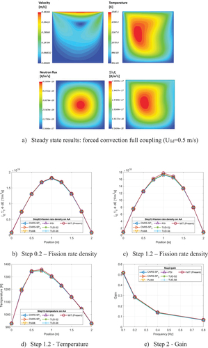
These results show good agreement with benchmark participants and exhibit maximum local differences of 9.8% of the fission reaction density in step 0.2, 7.1% of the local fission rate density and 1.0% of the local temperature in step 1.2, and 6.07% of gain in step 2. A majority of the discrepancy in each step is attributed to the neutronics model, six-group cross sections, and boundary settings adopted by participants.²⁴ It should be noted that in the present work, only a one-group diffusion solver is adopted. Another source of discrepancy could be from the different meshing strategy. Nevertheless, the current model demonstrates the ability to capture the dynamic behavior of LFMSRs.

III. REFERENCE MCFR MODEL

III.A. Description of the Reference MCFR Analysis Model

In the absence of some details of the reactor design and complete specifications for some of the components of the reference MCFR (Ref. 1), assumptions were made in the present study based on publicly available information in hopes of accurately simulating the characteristics of the finished reactor. Major design parameters for the reference MCFR are listed in Table I. The calculation domain of our reference MCFR model focuses on the core region to support the development of distributed in-core temperature monitoring with available computational resources. Influences from components in the primary loop, such as hot leg, cold leg, heat exchanger, and coolant salt in the intermediate loop, are included as a lumped model. The heat exchanger is assumed as a shell and tube–type having 115 tubes that are each 1 in. in diameter. The heat transfer coefficient is obtained from the Dittus-Boelter correlation.

TABLE I Design Parameters for the Reference MCFR Considered in the Present Study

Parameter	Value
Total thermal power	2500 MW(thermal)
Number of the primary loops	8
Fuel salt composition (in mol %)	65NaCl-35UCl3
Fuel salt in/out temperatures	923.14 K/1003.14 K
Diameter/length of hot leg and cold leg	0.5 m/2.0 m
Length of heat exchanger	2.5 m
Fuel salt transit time outside core	1.96 s
Average coolant salt temperature	823.14 K

Reactor geometry is assumed to consist of a cylindrical core with a diameter of 2 m and a height of 4 m. Reflectors consist of a 25-cm-thick lead radial reflector and elliptical lead axial top and bottom reflectors having a 0.5-m minor radius and a 1-m major radius. The vessel purports 15-cm-thick stainless steel walls. For the fuel salt, a eutectic mixture of 65 mol % NaCl and 35 mol % UCl₃ is specified. The thermophysical properties of the fuel salt derived from the literature^26–28 are listed in Table II. Neutronics data were generated by using SERPENT 2 (Ref. 29) to obtain the kinetic parameters of the DNPs, considering the 100%-enriched ³⁷Cl of the fuel salt. Six groups of DNPs were considered, which are defined in the ENDF/B-VII.0 nuclear data library. The temperature dependencies of the cross section and diffusion coefficient were derived by applying least-squares fitting on the calculated values at temperatures ranging from 600 to 1500 K.

TABLE II Fuel Salt and Structural Material Properties

	Fuel Salt	Lead	Stainless Steel
Density (kg/m^3)	4029.42	10284	8000
Specific heat (J/kg K)	476.86	145	500
Thermal conductivity (W/mK)	0.76	19.0	14.0
Viscosity (Pa s)	0.0011	–	–
Thermal expansion coefficient (1/K)	2.6E-04	–	–

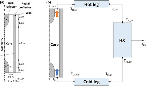
The CFD calculation domain for the reactor and schematic of the reference MCFR system considered in this study are shown in Figs. 2a and 2b, respectively. For the multiphysics simulation domain, a two-dimensional fluid/solid axisymmetric model was created representing one sector among eight primary loops in the reference MCFR design. Uniform inflow boundary conditions were set at the inlet surface with a velocity of 2.0 m/s and a temperature of 923 K. As the outside core region was not included in the multiphysics calculation, the amounts of incoming precursors after decay outside the core, C_in and D_in for DNPs and decay heat precursor, were set as uniform values of passive scalar calculated using Eq. (11)(11) $C_{i,in}\left(t\right)=C_{i,out}\left(t-{\tau }_L\right)e^{-{\lambda }_i{\tau }_L}\mathrm{a}\mathrm{n}\mathrm{d}{D}_{i,in}\left(t\right)=D_{i,out}\left(t-{\tau }_L\right)e^{-{\lambda }_{d,i}{\tau }_L}.$(11) and vacuum boundary conditions for the neutron flux. For the outlet, zero-gradient boundary conditions were set for velocity and temperature, DNPs and decay heat precursors, and vacuum boundary conditions for the neutron flux. The interfaces between regions were set as contact interfaces with conjugate heat transfer. As the neutronics calculation domain is limited to the core region only, albedo-type boundary conditions were adopted for the neutron flux and zero flux boundary conditions for the DNPs and decay heat precursors at the interfaces between the axial top and bottom reflectors and radial reflectors.

Fig. 2. Simulation domain of the reference MCFR: (a) reactor vessel dimension and (b) reference MCFR system.

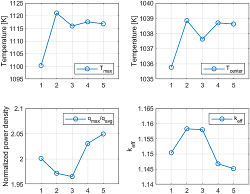
A quadrilateral mesh was used for the fuel salt, axial/radial reflector, and wall media using a direct mesh available in STARCCM+. A mesh convergence study was performed to find the proper grid configuration. Each mesh case was generated by decreasing the relative mesh scale in the x- and y-directions by a factor of 0.4 in the coarsest case (1) and increasing the scale by a factor of 2.6 in the finest case (5). All cases were run with anisotropic k-ε turbulence with wall distance y+ to 1 to capture the flow separation on the wall. As summarized in Fig. 3, mesh 4 showed sufficiently refined spatial distribution of the major parameters, so we selected mesh set 4 whose total number of cells is 173 400 for the present study.

Fig. 3. Mesh convergence results.

III.B. Steady-State Analysis

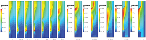
Figure 4 shows the steady-state velocity, temperature, neutron flux, delay neutron source, fission power density, and decay power density from left to right. Although the total power density and the sum of the fission power density and the decay power density are the highest at the core center, the temperature is actually relatively low due to the flow advection. Instead, a hot spot is created at the position where the flow separates near the axial bottom reflector. This phenomenon is evident in LFMSRs as the local temperature field is strongly related to the velocity field, which is governed by the core geometry. Such hot spots can be corrected in the design stage. Temperature distribution in the core can also be affected by radiative heat transfer (RHT) due to the high operating temperature of the system, although this effect is thought to be minimal. From our previous study, including an RHT model for the high-temperature fuel salt does not impact the temperature distribution significantly, while RHT marginally decreased the maximum temperature of the fuel salt by 3.0 K as expected.^9,30 As such, RHT modeling is not considered in the transient analysis for this work.

Fig. 4. Steady-state simulation results of the reference MCFR.

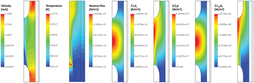
This motivates the use of distributed temperature monitoring of the reflector wall for validation of the multiphysics codes to support the LFMSR licensing basis. The original curved shape for the reflectors was motivated by minimization of the simulated flow separation. In practice, having such curvatures may be challenging from a structural engineering point of view and a flatter surface amplifies the observed temperature variation. Therefore, continuous monitoring of the temperature variation in real time along the reflector region can support structural lifetime and safety performance calculations for LFMSRs. We will later show that this can readily be accomplished with new single-crystal optical fiber temperature sensors.

IV. TRANSIENT BEHAVIOR OF A LFMSR

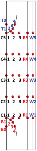
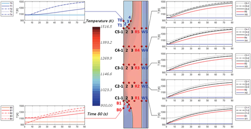
Major transients in LFMSRs are generally initiated by a malfunction of the pump in the primary loop or intermediate loop, which leads to a loss of heat sink or over cooling.¹⁷ Two types of transient scenarios are examined to provide the necessary performance basis of the advanced I&C for LFMSRs in the present study. One fault considered is unprotected, which means no mitigating actions are simulated, such as inserting reactivity control elements or activation of emergency cooling systems. The other transient considered is uniform perturbation of major system parameters, such as the fuel salt flow rate and the heat removal capability of the heat exchanger. All transients are simulated with the symmetric one-eighth portion of the reactor core with less computational resources. Steady-state solutions are used as initial conditions with scaling the fission operator by a factor of 1/k_eff to be critical at t = 0. The second-order implicit Euler scheme was chosen for the transient simulations using the time-step size of 0.001 s, which was chosen to yield a maximum Courant–Friedrichs–Lewy (CFL) less than 1.0. To track the temperature field variations during transients, monitoring points were selected at the core internal region, axial top and bottom reflector, and the radial reflector, as shown in Fig. 5.

Fig. 5. Locations of monitoring points.

IV.A. Unprotected Transients

To predict the operational range of the proposed distributed temperature sensor during transients, two scenarios were considered for the reference MCFR: loss of flow and loss of heat sink without power shutdown. Unprotected loss of flow (ULOF) is initiated by a failure of a pump in the primary loop. The ULOF was modeled as an exponential decrease of the fuel salt flow rate up to 20% of the nominal value with a time constant of 5.0 s, which is estimated using the relation in Eq. (15)(15) $Q\left(t\right)=Q\left(t_0\right)\left(0.8e^{-t/5}+0.2\right).$(15) :

(15) $Q\left(t\right)=Q\left(t_0\right)\left(0.8e^{-t/5}+0.2\right).$(15)

This is realistic given pump inertia and assumed natural circulation flow formation driven by the temperature difference between the primary loop and the intermediate loop.

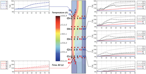
Figure 6 shows the transient response of the reference MCFR during ULOF. Reduction of the flow rate increases the net amount of DNPs existing in the core, introducing additional positive reactivity, while the increase of the overall temperature brings negative reactivity due to thermal feedback. The influence of the temperature increase dominates the DNP effect, resulting in a power decrease. Initially, when the fuel salt flow rate drops exponentially, drastic changes of the flow separation zone expand the high-temperature region to the core center, which results in an instant power increase from the temperature feedback. The hot spot initially at the bottom of the core moves upward to the top of the core ~50 s after the flow rate starts to decrease. The maximum core temperature reaches 1700 K at the top of the core adjacent to the axial upper reflector at around 80 s.

Fig. 6. Temperature evolution in the core during ULOF.

Figure 7 shows the temperature observed at monitored points in the fuel salt and core structures during ULOF. While the inlet temperature increases by only 20 K in 80 s, the top of the core region shows larger temperature changes. C5-1 shows the largest temperature change (435 K) among the monitoring points at the core center. Comparably, T2 and T3 on the axial top reflector show 435 and 446 K of temperature rise, respectively. At C2-1 to C5-2, the temperature of the fuel salt drops temporarily between 20 and 30 s due to negative power feedback from the increase of the fuel salt temperature, but the temperature at these locations increases shortly after that. As the flow rate decreases, the location of the hot spot moves toward the inlet as the recirculation zone reemerges. The monitoring points at the axial bottom reflector can capture this change. In locations like the core bottom where the flow rate changes significantly during an abnormal event, the temperature field also changes significantly. Monitoring the axial bottom reflector is appropriate for capturing these changes, while they cannot be captured by the monitoring points at the radial reflector and vessel wall.

Fig. 7. Local temperature evolution of the fuel salt and core components during ULOF.

The unprotected loss of heat sink (ULOHS) is the result of a reduction in the heat removal capabilities of the intermediate loop. The intermediate loop is represented by the average coolant salt temperature as described in Sec. III.B. To properly simulate this event sequence with the existing model, we represented a ULOHS scenario by an exponential increase of the coolant salt temperature up to 120% of its nominal value and an exponential reduction of the heat transfer coefficient of the heat exchanger in the primary loop up to 80% of its nominal value, simultaneously with the time constant of 5 s as shown in Eqs. (16)(16) $T_{cs}\left(t\right)=T_{cs}\left(t_0\right)\left(1.2-0.2e^{-t/5}\right)$(16) and (17(17) $h\left(t\right)=h\left(t_0\right)\left(0.8e^{-t/5}+0.2\right).$(17) ):

(16) $T_{cs}\left(t\right)=T_{cs}\left(t_0\right)\left(1.2-0.2e^{-t/5}\right)$(16)

and

(17) $h\left(t\right)=h\left(t_0\right)\left(0.8e^{-t/5}+0.2\right).$(17)

Figure 8 shows the time response of the reference MCFR during ULOHS. The inlet temperature starts to rise as the heat removal capability drops, and the temperature of the heat exchanger and the cold leg begin to increase. In the first ~12 s, the magnitude and the location of the core maximum temperature remains the same. At ~13 s, the hot spot moves upward to the axial top reflector. The maximum temperature of the fuel salt reaches 1500 K at the top of the core at around 72 s. After 80 s, the system almost reaches the new steady state at around 80% of total power and 1420 K fuel salt average temperature.

Fig. 8. Temperature evolution in the core during ULOHS.

Figure 9 shows the simulated temperature at the monitored fuel salt and core structure points during ULOHS. The inlet temperature increases by 500 K, while the heat removal capability reaches 20% of the nominal value at 80 s. Unlike ULOF, fuel salt temperatures rise homogeneously, irrelevant of the position. As such, the monitoring points on the radial reflector can observe the fuel salt temperature increase. B2, B3, and B4 on the axial bottom reflector near the inlet and T3 and T4 on the axial top reflector near the outlet also follow the trends of temperature variations in the adjacent fuel salt. B1 and T1, located at the core center, show a relatively slow thermal response. As expected in ULOF, B0 and T0 do not track the fuel salt temperature variations as well.

Fig. 9. Local temperature evolution of the fuel salt and core components during ULOHS.

Table III summarizes the maximum temperature changes of the core components during 80 s of ULOF and ULOHS. The power level drops and reaches a new steady state at 88% and 80% of the nominal power in the ULOF and ULOHS scenarios after 80 s, respectively, due to negative power feedback from the fuel salt temperature increase. Although the amount of the power change in ULOF is smaller than that in ULOHS, the maximum temperature of the fuel salt increases by 550 K during ULOF in 80 s, compared to 400 K during ULOHS. Flow field variations during ULOF influence the local temperature field in the core, mainly near the recirculation zone and the core top region. On the other hand, the fuel salt temperature field is strongly dependent on the inlet temperature variations during ULOHS. Since local temperature variations are less affected by the radial reflector during ULOF, the radial reflector temperature increases by only 133 K in the ULOF scenario, while the radial reflector temperature increases 292 K during ULOHS. In both cases, the maximum temperature of the vessel wall does not change for the first 80 s.

TABLE III Maximum Temperature of the Core Components at 80 s During Unprotected Transients

	Steady State	ULOF	ULOHS
Fuel salt in core	1117.21 K	1666.90 K	1516.67 K
Axial bottom reflector	1115.78 K	1353.35 K	1441.09 K
Axial top reflector	1075.18 K	1515.51 K	1476.49 K
Radial reflector	976.14 K	1109.36 K	1267.76 K
Vessel wall	976.05 K	976.05 K	976.05 K

IV.B. Uniformly Perturbed Transients

To inform necessary temporal and thermal resolution of the proposed distributed temperature sensing system, the thermal response from uniform perturbations of the fuel salt flow rate and the heat removal capability were investigated. Perturbed transients were modeled as a sinusoidal oscillation by multiplying the temporal function f to the fuel salt flow rate and the coolant salt temperature, expressed as a sine wave of amplitude 20% and period p of 0.5, 1.0, 2.5, and 5.0 s, as indicated by Eq. (18)(18) $f=1+0.2sin\left(\frac{2\pi }{p}t\right).$(18) :

(18) $f=1+0.2sin\left(\frac{2\pi }{p}t\right).$(18)

Uniformly perturbed transients were simulated until a stable trend emerged. To configure the thermal response rate at each measuring position, time derivatives of the temperature were obtained by using a first-order central difference approximation in time, as in Eq. (19)(19) ${\left(\frac{dT}{dt}\right)}^i=\frac{T^{i+1}-T^{i-1}}{2\mathrm{\Delta }t}.$(19) :

(19) ${\left(\frac{dT}{dt}\right)}^i=\frac{T^{i+1}-T^{i-1}}{2\mathrm{\Delta }t}.$(19)

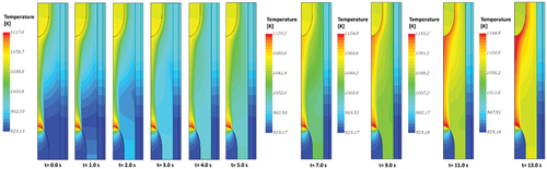
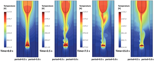
During flow rate perturbation transients, the temperature of each component follows the sinusoidal flow rate oscillation in the first 5 s. Shortly after, the temperature starts to rise due to the temporal variations in the power from the inflow of DNPs after the first circulation, which act as a reactivity insertion. Then strong negative feedback following the temperature rise drops the power level and the temperature oscillates along with the flow rate variations. As shown in Fig. 10, thermal stratification is observed near the core center from the velocity field oscillation starting at the lower core region for both perturbation periods of 0.5 and 5.0 s. The position where the flow separation starts moves back and forth to the core center as the flow rate varies, which forms the distinct wavy region. It promotes thermal mixing of the fuel salt in the core, and the temperature field in the core becomes flatter.

Fig. 10. Comparison of temperature evolution during flow rate fluctuation transients for the periods of 0.5- and 5.0-s cases.

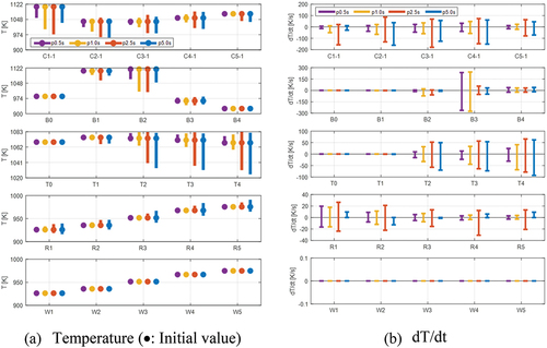
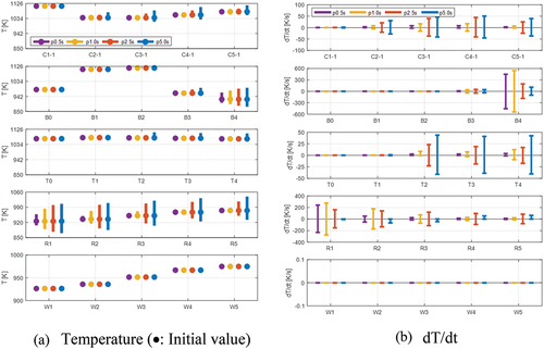
Figure 11 summarizes the global maximum and minimum temperature and the rate of temperature change of the fuel salt at the core center for structural materials during flow rate perturbed transients. The temperature of the fuel salt in the core center eventually drops as local thermal mixing is enhanced by flow field oscillation. The range of temperature variation on the radial reflector slightly increases as the period gets longer, but the temperature of all monitoring points on the vessel wall remains the same regardless of the period. The rate of temperature change at the monitoring points on the axial top reflector showed a maximum value of 93 K/s at T4 near the outlet with a 5.0-s period, which is similar to the hot leg temperature changes. Similar to unprotected transients, the thermal response of W1 to W5 on the vessel wall is imperceptible during flow rate fluctuation transients regardless of the period. At the axial bottom reflector, the influence of the flow field oscillation on the temperature depends on the exact location being monitored. B2 on the axial bottom reflector has a maximum temperature variation of 109 K, and it undergoes a 73 K/s rate of temperature change with a 1.0-s perturbation period. In contrast, B3 exhibits only a 38-K temperature rise but exhibits a maximum rate of change of 276 K/s. The largest rate of temperature change (276 K/s) is noted to occur at B3 (followed by 180 K/s at C3-1) with a perturbation period of 1.0 s. The rate of temperature change on the radial reflector is also in agreement with that of the core center at C1-1 to C1-5, but the magnitude is smeared out away from the core center.

Fig. 11. Temperature range and temporal temperature change of reactor structures during flow rate fluctuation transients: (a) temperature (•: initial value) and (b) dT/dt.

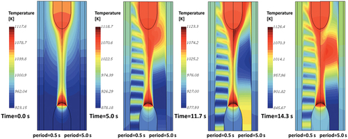
Next, during inlet temperature fluctuation transients, the inlet temperature change during heat sink capability oscillations instantly affects the local temperature field in the core region, which is the greatest influencing factor on the power density and overall temperature. Since the velocity field in the core region remains the same as the initial velocity field in this case, the position of the hot spot at the axial bottom reflector does not change and hot spot formation is mainly due to the flow separation. The overall temperature range during the heat sink fluctuation transients is determined by the amplitude and the period of the cold leg temperature variations. The overall temperature ranged from 877 to 1005 K with a 0.5-s period and from 840 to 1037 K for a 5.0-s period. The local temperature field forms a distinct pattern inside the entire core area as the inlet temperature oscillates, which propagates until the oscillating fuel salt reaches the outlet as shown in Fig. 12. This can be contrasted with the local wavy pattern that is formed at the center of the core during flow rate fluctuation transients.

Fig. 12. Temperature evolution during heat sink fluctuation transients.

Figure 13 summarizes the global maximum and minimum temperature and corresponding rate of temperature change of the fuel salt at the core center and structural materials during heat sink capability oscillations. Compared to the flow rate fluctuation transients, the average temperature of the fuel salt at the core center remains at the initial value, and the amount of temperature variation becomes larger in long-period cases. B4 on the axial bottom reflector exhibits a trend similar to the inlet temperature variations, showing a maximum rate of temperature change of 600 K/s for a period of 1.0 s. Measurement points at B1 and B2 close to the core internal region exhibit a smaller rate of temperature change than those near the inlet. All measurement points on the axial top reflector, except T0, show similar temperature variations and rates of temperature change. Unlike the flow rate fluctuation transients, fuel salt temperature variations during heat sink fluctuation transients can be tracked at the radial reflector. R1 shows the largest rate of temperature change (250 K) for a period of 1.0 s, which grows smaller and smaller closer to the outlet. As with the flow rate fluctuation transients, the vessel wall temperature is the same as its initial value during heat sink fluctuation transients.

Fig. 13. Temperature range and temporal temperature change of reactor structures during heat sink fluctuation transients.

From the results of modeling unprotected and uniformly perturbed transients, it is clearly seen that temperature transients in the fuel salt smooth out as we move radially outward in the reactor toward the vessel wall. Temperatures monitored at the surface of the axial reflectors can capture the trends of the temperature variations in the fuel salt in the core. Temperature measurements at the axial top reflector can be used to track reactor maximum temperatures. However, both the temperature of T0 and B0, located in the middle of the axial top and bottom reflector, remain the same for all transients due to the large thermal mass of the structures and high temperature gradients near the walls. Therefore, temperature measurement sensors need to be installed such that the measurement of the entire reflector temperature distribution in contact with the salt is possible. This implies measurement by traditional pointwise thermocouples or other single-point sensors is not sufficient for monitoring complex MSR system temperatures where transients may occur frequently. As we have also noted, in order to capture realistic transients that are expected to occur quickly, a temperature sensor system with a reasonably high acquisition speed (1 Hz or greater) must be implemented. In addition, it is known that temperature changes as low as 50 K in chloride salts can double the rate of corrosion, particularly at these high temperatures.³¹ Moreover, cyclical thermal loads induce mechanical loads on the structures, resulting in structural failures. Therefore, regions where a large temperature variation is expected (such as the radial reflector) should be monitored with high temporal and spatial resolution to evaluate the structural integrity and amount of expected fatigue or corrosion over time. This can be enabled with the use of new distributed fiber-optic sensors to support the structural lifetime and safety performance of a LFMSR, as discussed in Sec. V.

V. DISCUSSION ON USE OF DISTRIBUTED SENSING TECHNOLOGY

From the data generated in this modeling effort, several important conclusions about LFMSR sensor design and placement can be garnered. First, we note that single-point temperature sensors are not adequate for the measurement of complex reactor operations and cannot give a clear picture of the transients likely to result from common operational failure modes and perturbations. This leads us to the possibility of performing distributed or wide-area sensing inside LFMSR cores. Unfortunately, most conventional wide-area sensor systems are hampered by high radiation loads that result in short sensor-system lifetimes or erroneous measurement results. Second, we note that the rate at which some common transient events are expected to occur implies the need for a sensor system that performs at a relatively fast measurement rate. Rates of around 1 Hz are required to measure most relevant transients, and higher rates are desirable for tracking minor excursions. Finally, we note that due to the fast nature of these events and the corrosion rate dependence on temperature, a high degree of temperature accuracy is required. While resolution in the 1°C range is desirable, it may be possible to monitor a majority of events with a 2°C to 5°C resolution. The need for a sensor system with high spatial resolution, high thermal accuracy, and fast response time should be implemented for the optimization of reactor operating parameters, the estimation of component lifetimes, and for providing automated system operation stabilization during transient events.

Distributed fiber-optic sensing is a likely candidate to provide in-core sensing, which has been studied by a number of groups.³² With recent advances in single-crystal fiber optics that employ materials like sapphire and yttrium aluminum garnet as the fiber core material, it is becoming evident that single-crystal fibers may be capable of surviving the harsh MSR core environment.³³ Using single-crystal fibers may provide the key to realizing distributed temperature or multi-parameter sensing in a core environment while employing a single core penetration feedthrough and a distributed optical interrogator based on optical scattering phenomena. Recently, an optical interrogator was constructed for use with single-crystal optical fibers based on the Raman scattering principle.³⁴ This interrogator is being field tested with single-crystal optical fibers grown via the laser-heated pedestal growth method for applications in nuclear energy, including LFMSRs and traditional light water reactors. Such a system could provide the means to conduct the necessary measurements desirable for reactor monitoring and control or to potentially provide more immediate utility supporting the licensing basis for new reactor designs through model validation and scale-up verification at the pilot stage.

VI. CONCLUSIONS

A multiphysics simulation tool for analyzing LFMSRs was presented to inform the implementation of advanced I&C using fiber optics for supporting the safety basis of LFMSRs. A neutronics calculation module was implemented in passive scalar transport form using the commercial CFD software STAR-CCM+. The module was based on the one-group diffusion theory for the neutron flux and DNPs and decay heat precursor balance equations considering the drift due to the flow. System components, such as the heat exchanger, the hog leg, and the cold leg, were modeled using the lumped method based on the energy balance. The tool in the present work was verified by showing good agreement to the benchmark problem developed for evaluating coupling methodologies for the neutronics and thermal hydraulics of various solvers for MSFR analysis. A two-dimensional axisymmetric model of the reference MCFR design was simulated in the steady state and was applied to abnormal events such as the unprotected and the uniformly perturbed scenarios shown here. These events were simulated to provide desired performance metrics for distributed temperature sensing.

Steady-state results showed a strong dependency of the temperature field on the flow field determined by the curved shape of the core geometry. The shape was originally intended to minimize the flow separation, which is challenging from an engineering point of view. A flatter surface, adopted widely in practical applications, is expected to amplify the observed temperature variation. This motivates the use of the distributed monitoring of the reflector wall for validation of the multiphysics code to support the LFMSR licensing basis. The results of the unprotected transients and uniformly perturbed transients show the limitations of conventional pointwise temperature measurements and emphasize the importance of continuous temperature monitoring of the core structure. During flow rate variation–driven transients, such as ULOF and flow rate fluctuations, localized variations of the temperature were observed near the hot spot located at the recirculation zone. In this case, monitoring points on the axial reflector were able to capture the thermal response of the reactor during transients. Temperature variation–driven transients, such as ULOHS and heat sink capability fluctuations, showed dependency on the inflow fuel salt temperature. In this case, monitoring points on the radial reflector were able to track the fuel salt temperature variation. For all cases, temperature signals in the core smoothed out going toward the reflector and vessel walls, where no change in the temperature was observed. Since temperature changes in chloride molten salts as small as 50 K can double the rate of corrosion,³¹ particularly in the high-temperature range typical in MSR operating conditions, continuous monitoring of the temperature variation in real time along the reflector region can support the structural lifetimes and safety performance basis for LFMSRs, which can be readily enabled with the use of fiber optics.

The capabilities of the multiphysics tool presented here based on the CFD methodology coupled with a neutronics solver can give insights to formulate operational metrics for the development of advanced I&C technology to support the licensing basis of LFMSRs in any complex reactor geometry. The present model can solve complex thermal-hydraulic problems with preimplemented turbulence models to obtain three-dimensional distributions of the temperature, velocity, and neutron flux, and the distribution of the DNPs in various conditions given any new LFMSR design. It is concluded that the framework of the present model can give physical insight into understanding the complex behavior of LFMSRs and can be applied as a tool for the development of advanced I&C to support the safety basis for LFMSRs.

Disclosure Statement

No potential conflict of interest was reported by the authors.

Additional information

Funding

This work is supported by the U.S. Department of Energy ARPA-E project (DE-AR00001154).

References

- “MCFR TerraPower,” TerraPower; http://terrapower.com/technologies/mcfr (current as of Feb. 25, 2022).
- “Moltex Energy,” SSR TECHNOLOGY; https://www.moltexenergy.com/technology-suite (current as of Feb. 25, 2022).
- D. E. HOLCOMB, R. A. KISNER, and S. M. CEITNER, “Instrumentation Framework for Molten Salt Reactors,” ORNL/TM-2018/868, Oak Ridge National Laboratory (June 2018).
- P. F. PETERSON et al., “Integral and Separate Effects Tests for Thermal Hydraulics Code Validation for Liquid-Salt Cooled Nuclear Reactors,” Compact Integral Effects Test (CIET) Final Report, Project Number 09-789 (October 2012).
- A. CAMMI et al., “A Multi-Physics Modelling Approach to the Dynamics of Molten Salt Reactors,” Ann. Nucl. Energy, 38, 6, 1356 (2011); https://doi.org/10.1016/j.anucene.2011.01.037.
- H. ROUCH et al., “Preliminary Thermal-Hydraulic Core Design of the Molten Salt Fast Reactor (MSFR),” Ann. Nucl. Energy, 64, 449 (2014); https://doi.org/10.1016/j.anucene.2013.09.012.
- B. FENG et al., “Multiphysics Modeling of Precursors in Molten Salt Fast Reactors Using Proteus and Nek5000,” Proc. PHYSOR2020, Cambridge, United Kingdom, March 28–April 2, 2020, EPJ Web of Conference (2020).
- M. RAMZY ALTAHHAN et al., “Preliminary Design and Analysis of Liquid Fuel Molten Salt Reactor Using Multi-Physics Code GeN-Foam,” Nucl. Eng. Des., 369, 110826 (2020); https://doi.org/10.1016/j.nucengdes.2020.110826.
- Y. JEONG and K. SHIRVAN, “Multiphysics Modeling of Fast Liquid-Fuel Molten Salt Reactor Using STAR-CCM+,” Proc. M&C 2021, October 3–7, 2021, American Nuclear Society ( 2021).
- M. AUFIERO et al., “Development of an OpenFOAM Model for the Molten Salt Fast Reactor Transient Analysis,” Chem. Eng. Sci., 111, 390 (2014); https://doi.org/10.1016/j.ces.2014.03.003.
- A. LINDSAY et al., “Introduction to Moltres: An Application for Simulation of Molten Salt Reactors,” Ann. Nucl. Energy, 114, 530 (2018); https://doi.org/10.1016/j.anucene.2017.12.025.
- F. CARUGGI et al., “Multiphysics Modelling of Gaseous Fission Products in the Molten Salt Fast Reactor,” Nucl. Eng. Des., 392, 111762 (2022); https://doi.org/10.1016/j.nucengdes.2022.111762.
- A. DI RONCO et al., “Multiphysics Analysis of RANS-Based Turbulent Transport of Solid Fission Products in the Molten Salt Fast Reactor,” Nucl. Eng. Des., 391, 111739 (2022); https://doi.org/10.1016/j.nucengdes.2022.111739.
- G. YANG et al., “Development of Coupled PROTEUS-NODAL and SAM Code System for Multiphysics Analysis of Molten Salt Reactors,” Ann. Nucl. Energy, 168, 108889 (2022); https://doi.org/10.1016/j.anucene.2021.108889.
- J. GROTH-JENSEN et al., “Verification of Multiphysics Coupling Techniques for Modelling of Molten Salt Reactors,” Ann. Nucl. Energy, 164, 108578 (2021); https://doi.org/10.1016/j.anucene.2021.108578.
- A. LAUREAU et al., “Transient Coupled Calculations of the Molten Salt Fast Reactor Using the Transient Fission Matrix Approach,” Nucl. Eng. Des., 316, 112 (2017); https://doi.org/10.1016/j.nucengdes.2017.02.022.
- M. TIBERGA, “Development of a High-Fidelity Multi-Physics Simulation Tool for Liquid-Fuel Fast Nuclear Reactors,” PhD Thesis, TU Delft University, Energy and Nuclear Engineering (2020).
- H. LIAOYUAN et al., “Th-U Breeding Performances in an Optimized Molten Chloride Salt Fast Reactor,” Nucl. Sci. Eng., 195, 2, 185 (2020); https://doi.org/10.1080/00295639.2020.1798728.
- R. T. COYLE, T. M. THOMAS, and G. Y. LAI, “Exploratory Corrosion Tests on Alloys in Molten Salts at 900°C,” J. Mater. Energy Syst., 7, 4, 345 (1986); https://doi.org/10.1007/BF02833573.
- W. DING, A. BONK, and T. BAUER, “Corrosion Behavior of Metallic Alloys in Molten Chloride Salts for Thermal Energy Storage in Concentrated Solar Power Plants: A Review,” Front. Chem. Sci. Eng., 12, 3, 564 (2018); https://doi.org/10.1007/s11705-018-1720-0.
- A. CAMMI et al., “Dimensional Effects in the Modelling of MSR Dynamics: Moving on from Simplified Schemes of Analysis to a Multi-Physics Modelling Approach,” Nucl. Eng. Des., 246, 12 (2012); https://doi.org/10.1016/j.nucengdes.2011.08.002.
- M. S. GREENWOOD and B. BETZLER, “Modified Point-Kinetics Model for Neutron Precursors and Fission Product Behavior for Fluid-Fueled Molten Salt Reactors,” Nucl. Sci. Eng., 193, 4, 417 (2019); https://doi.org/10.1080/00295639.2018.1531619.
- STAR-CCM+ 13.06 Software Manual, Siemens (2018).
- M. TIBERGA et al., “Results from a Multi-Physics Numerical Benchmark for Codes Dedicated to Molten Salt Fast Reactors,” Ann. Nucl. Energy, 142, 107428 (2020); https://doi.org/10.1016/j.anucene.2020.107428.
- D. WOOTEN and J. J. POWERS, “A Review of Molten Salt Reactor Kinetics Models,” Nucl. Sci. Eng., 191, 3, 203 (2018); https://doi.org/10.1080/00295639.2018.1480182.
- V. N. DESYATNIK et al., “Density, Surface Tension, and Viscosity of Uranium Trichloride-Sodium Chloride Melts,” At. Energiya, 39, 1, 70 (1975).
- S. KATYSHEV and L. TESLYUK, “Ionic Melts in Nuclear Power,” in Challenges and Solutions in the Russian Energy Sector, pp. 181–189, Springer (2018).
- M. TAUBE and J. LIGOU, “Molten Plutonium Chlorides Fast Breeder Reactor Cooled by Molten Uranium Chloride,” Ann. Nucl. Sci. Eng., 1, 277 (1974); https://doi.org/10.1016/0302-2927(74)90045-2.
- “Serpent—A Monte Carlo Reactor Physics Burnup Calculation Code”; http://montecarlo.vtt.fi/ (current as of Feb. 10, 2021).
- C. COYLE, E. BAGLIETTO, and C. FORSBERG, “Advancing Radiative Heat Transfer Modeling in High-Temperature Liquid Salts,” Nucl. Sci. Eng., 194, 8–9, 782 (2020); https://doi.org/10.1080/00295639.2020.1723993.
- J. C. GOMEZ-VIDAL and R. TIRAWAT, “Corrosion of Alloys in a Chloride Molten Salt (NaCl-LiCl) for Solar Thermal Technologies,” Solar Energy Mater. Sol. Cells, 157, 234 (2016); https://doi.org/10.1016/j.solmat.2016.05.052.
- P. LU et al., “Distributed Optical Fiber Sensing: Review and Perspective,” Appl. Phys. Rev., 6, 041302 (2019); https://doi.org/10.1063/1.5113955.
- M. BURIC et al., “Modified Single Crystal Fibers for Distributed Sensing Applications,” Proc. SPIE 10208, Fiber Optic Sensors and Applications XIV, p. 102080C (Apr. 27, 2017); https://doi.org/10.1117/12.2262992.
- B. LIU et al., “Design and Implementation of Distributed Ultra-High Temperature Sensing System with a Single Crystal Fiber,” J. Light. Technol., 36, 23, 5511 (2018); https://doi.org/10.1109/JLT.2018.2874395.