Parametric Model-Order Reduction for Radiation Transport Simulations Based on an Affine Decomposition of the Operators

Abstract

This work presents a data-driven, projection-based parametric reduced-order model (ROM) for the neutral particle radiation transport (linear Boltzmann transport) equation. The ROM utilizes the method of snapshots with proper orthogonal decomposition. The novelty of the work is in the detailed proposal to exploit the parametrically affine transport operators to intrusively, yet efficiently, build the reduced transport operators in real time in a matrix-free manner compatible with sweep-based transport solvers. This affine-based ROM is applied to one-dimensional (1-D), two-dimensional (2-D), and 2-D multigroup transport benchmarks and is found to significantly outperform less intrusive ROMs in terms of speed for a desired accuracy level. The ROM has an 18.2 to 89.4 speedup with an error range of 0.0002% to 0.01% for the 1-D benchmark, a 1120× to 4870× speedup with an error range of 0.0009% to 0.01% for the 2-D benchmark, and a 54 600× to 399 800× speedup with an error range of 0.00022% to 0.01% for the multigroup 2-D benchmark. Even higher speedups are expected for three-dimensional multigroup transport problems.

Keywords:

• Proper orthogonal decomposition
• model-order reduction
• reduced-order models
• radiation transport
• affine decomposition

I. INTRODUCTION

As computing power has increased over the past decades, so has the complexity of the models used to represent physical systems in science and engineering. Faster processors, larger memory banks, and increased parallel capabilities have enabled numerical simulations that mimic natural phenomena with finer details. However, these high-fidelity simulations, or full-order models (FOMs), may come at a high computational cost in terms of both CPU time and memory. This is the case for radiation transport simulations that typically require the solution of the linear Boltzmann transport equation. The Boltzmann equation needs to be discretized along six phase-space dimensions—space (3), angle (2), and energy (1)—as well as in time for unsteady problems. The resulting discretizations yield very large linear systems of equations, with up to 10¹⁴ degrees of freedom, that must be solved to obtain the transport solution^1–3 and any desired quantities of interest (QoIs) and functionals of the solution itself. Furthermore, these simulations are often parametric in so far that the solution is dependent on a set of input or uncertain parameters that characterize the problem. Such varying parameters may include material cross sections, source terms, boundary conditions, and problem geometry. Therefore, in applications such as (1) design optimization and (2) uncertainty quantification, high-fidelity solutions are often required for many parameter realizations, resulting in a computationally demanding if not prohibitive task. Furthermore, the time required to solve such large systems can render simulations useless for real-time or near real-time applications.

Model-order reduction (MOR) is a technique aimed at reducing the computational complexity of numerical simulations.^4–7 A parametric reduced-order model (ROM) aims to accurately emulate, with an acceptable computational cost, the input parameter/output solution mapping of the high-fidelity model (FOM). This ROM is then used to inexpensively obtain solutions for any parameter realization relevant to the problem application.

This work discusses a data-driven, projection-based ROM for radiation transport that utilizes proper orthogonal decomposition (POD) for subspace discovery and affine decomposition to obtain the modal expansion coefficients in the learned subspace. The ROM is intrusive in that it requires access to the FOM’s source code. However, the method exploits the affine nature of the transport operator with respect to the input parameter in order to offer significant speedups compared to other less intrusive methods.

There are many variants of ROMs, such as physics-based, data-driven, intrusive, and nonintrusive methods, to name a few. Diffusion is perhaps the most well-known physics-based ROM for radiation transport. The diffusion approximation reduces the dimensionality of the FOM by two by eliminating the angular portion of the phase space.⁸ When performing parametric analyses and uncertainty quantification on QoIs, adjoint theory⁹ is an effective ROM that provides first-order sensitivity. Polynomial chaos expansion (PCE) is a technique that expands parametric QoIs as a series of orthonormal polynomials with both intrusive and nonintrusive options.¹⁰ Once the PCE coefficients have been obtained, a ROM may be quickly queried to obtain QoIs for all parameter values. Within the nuclear engineering community, PCE has found applications in radiation diffusion,¹¹ radiation transport,^12,13 point-kinetics,¹⁴ and criticality¹⁵ problems. Proper generalized decomposition (PGD) is another function expansion ROM that seeks the FOM solution as the sum of the product of one-dimensional (1-D) functions of each variable in the phase space. Thus, while the cost to solve the FOM increases exponentially with dimension, the cost to solve the ROM increases only linearly. PGD has been used for neutron diffusion^16–19 and transport.^20,21 As with PCE, a PGD ROM may be quickly queried to obtain parametric solutions after it is built. Dynamic mode decomposition (DMD) is a data-driven method used to capture the dynamics of a system while preserving its eigenvalues. Used in computational fluid dynamics,^22–24 DMD has made its way into nuclear engineering with applications in diffusion²⁵ and transport.²⁶ Parametric versions of DMD have recently been developed.^27,28 There are numerous other categories of ROMs outside of this review, such as Krylov subspace techniques,^29,30 autoencoders (neural networks),³¹ and Gaussian processes.³²

This work utilizes a data-driven, projection-based ROM that is based on POD. POD was devised in 1901 with Karl Pearson’s work³³ and is often referred to under different, domain-specific names, such as the method of empirical orthogonal functions in geophysics,³⁴ principal component analysis in statistics,³⁵ and Karhunen–Loève expansion in other disciplines.³⁶ Applications of POD are widespread, from the medical field³⁷ to mechanical modeling^38,39 to fluid dynamics.^40–46 Although POD ROMs typically seek the best approximation to the FOM solution in a least-squares sense, there are versions supplemented with adjoint theory that seek to optimize the reduced solution in the regions of interest (RoIs) containing the QoIs (Ref. 47). Within nuclear engineering, POD has been used to reduce diffusion k-eigenvalue problems,^48,49 transport problems,^50–55 and reactor kinetics problems.^56,57 Within these references, there has been some noteworthy progress in the area of POD applied to radiation transport. Buchan et al.⁵⁰ and Hughes and Buchan⁵¹ have applied the method to two-dimensional (2-D) monoenergetic transport and have obtained ROM speedups of up to two orders of magnitude. Coale⁵⁸ tested the method on multigroup transient transport in 1-D purely absorbing slabs. Finally, Tencer et al.^52,53 have applied POD to monoenergetic transport in pure absorbing media in three dimensions. They treated the particle direction as parametric and used FOM solutions for a few discrete directions to build a ROM to predict transport solutions for any arbitrary direction. Additionally, they briefly state that they utilized an affine form of the transport operator to efficiently build the reduced operators, a powerful method that is little discussed in the transport community. Sun et al.⁵⁵ proposed a POD ROM for the angular flux in S_N radiation transport. However, they did not exploit the affine decomposition of the transport operators and showed a speedup factor of about 29.

The projection-based ROM seeks to reduce the dimensionality of the FOM by seeking the discretized solution as a linear combination of basis vectors. The subspace that the basis vectors span is determined during a data-driven offline learning phase. During the data collection phase, the parameter space is adequately sampled and the FOM solutions, or snapshots, are computed for all sample (training) points. Next, POD is performed by computing the singular value decomposition (SVD) of the snapshot data to obtain the aforementioned basis vectors, or POD modes. SVD minimizes the distance between the FOM and ROM solutions for the snapshot data set in an least-squares sense.⁵⁹ The POD modes are ordered by decreasing variance, with each mode describing some characteristics of the system.³⁵ With the basis vectors determined, the POD mode expansion approximation is substituted into the transport equation and projected onto the learned subspace, yielding a small (relative to the FOM) parametric system to be solved for the modal coefficients in the online prediction phase. With the coefficients in hand, the approximation to the FOM is obtained by evaluating the linear combination of basis vectors.

To be useful, the computational expense of evaluating a parametric ROM in the prediction phase should be far less than that of solving the FOM itself. In this study, the handling of the projection portion determines whether the ROM is fast enough to be of practical use. We denote the size of the FOM solution vector by $N$ and that of the ROM solution vector by $r$, where, typically $r<<N$. The projection step leads to a small $r\times r$ system of equations that needs to be solved for the expansion or modal coefficients. However, this often involves operations with full-size arrays (of length $N>>r$) and this can be costly. The key to a practically useful ROM is in the efficient computation of that reduced system of equations, including in situations where the reduced operator depends on parametric variables. However, large radiation transport FOMs are often solved using a matrix-free approach (known as mesh sweeping or transport sweeps), whereby the full-order operator is never built due to the large number of phase-space unknowns.^1–3 Not having direct access to the full-order operator can make the ROM projection step costly and ineffective, thereby reducing the usefulness of ROMs for transport sweep–based FOMs. For instance, ROMs for transport sweep–based radiation transport was proposed in Refs. 60 and 61, but they have yielded marginal speedups over the FOM for two reasons: (1) the ROMs were minimally invasive, thus the projection step for any new parametric value required the action of the full-order transport operator (i.e., a transport sweep) on the POD modes, and (2) the ROMs were devised for the flux moments (of which the scalar flux is the lowest order) and the sweep preconditioner made the transport operator not affine in the parameters.

In this present work, we devise a ROM approach that is compatible with an affine decomposition of the full-order transport operator and compare this new approach against the minimally invasive sweep-based ROMs. When an operator $A(\mu )$ is affine with respect to its parameters $\mu$, the operator may be decomposed into a sum of scalar parametric functionals $f_i(\mu )$ multiplied by size $N\times N$ parameter-independent operators $A_i$:

$A(\mu )=\sum _i{f}_i(\mu )A_i.$

Therefore, the projection step of MOR can be performed on the parameter-independent operators $A_i$, as a preprocessing stage before any parameter realizations are drawn.⁶² Both German and Ragusa⁴⁸ and Heaney et al.⁶³ used an affine decomposition of the multigroup neutron diffusion equations for k-eigenvalue problems. However, the affine decomposition approach is, so far, seldom used in parametric ROMs for radiation transport, with the exception of the work in Refs. 64 and 65. In spite of this lack of usage for transport applications, other disciplines have utilized affine decomposition of operators in ROMs through linearization techniques.^62,66 Although an affine transport representation allows for efficient computation of the projection terms, resulting in high ROM speedups, it can come with two disadvantages. First, the ROM is intrusive in that it requires access to the FOM source code in addition to the new source code that must be written to compute the parameter-independent portions of the projection terms. Second, the affine transport operators are written in terms of the higher dimensional angular flux variable instead of the flux moments. This requires that snapshots and POD modes be saved as angular fluxes, increasing file space and memory requirements over less intrusive ROMs that only work with flux moment quantities. However, application of an affine-decomposed ROM to 1-D (Ref. 64) and 2-D (Ref. 65) transport problems have yielded promising results.

The remainder of this work is as follows. First, Sec. II gives an overview of the radiation transport FOM. Next, Sec. III discusses how the ROM is built and applied to the parametrically affine transport operators. Section IV applies the ROM to several parametric transport benchmarks to evaluate its performance. Finally, Sec. V summarizes the method and the authors’ findings.

II. FOM: NEUTRAL RADIATION TRANSPORT

The linear Boltzmann equation, or radiation transport [see Eq. (8(8) $N_{\varphi }=G\times N_{\mathrm{m}\mathrm{o}\mathrm{m}}\times I.$(8) )], is a statement of particle conservation that can be expressed as

(1a) $\begin{array}{rl}& \vec{\mathrm{\Omega }}\cdot \vec{\mathrm{\nabla }}\psi (\vec{r},E,\vec{\mathrm{\Omega }})+{\mathrm{\Sigma }}_t(\vec{r},E)\psi (\vec{r},E,\vec{\mathrm{\Omega }})\\ & ={\int }_{4\pi }d\mathrm{\Omega }\prime {\int }_0^{\mathrm{\infty }}dE\prime {\mathrm{\Sigma }}_s(\vec{r},\hspace{0.17em}E\prime \to E,\vec{\mathrm{\Omega }}\prime \to \vec{\mathrm{\Omega }})\psi (\vec{r},E\prime ,\vec{\mathrm{\Omega }}\prime )+Q(\vec{r},E,\vec{\mathrm{\Omega }}),\mathrm{\forall }\vec{r}\in \mathcal{D}\end{array}$(1a)

and

(1b) $\begin{array}{rl}& \psi (\vec{r},E,\vec{\mathrm{\Omega }})={\psi }_{\mathrm{i}\mathrm{n}\mathrm{c}}(\vec{r},E,\vec{\mathrm{\Omega }})\\ & \mathrm{\forall }\vec{r}\in \mathrm{\partial }{\mathcal{D}}^{-}=\left\{\vec{r}\in \mathrm{\partial }\mathcal{D}\mathrm{s}\mathrm{u}\mathrm{c}\mathrm{h}\mathrm{t}\mathrm{h}\mathrm{a}\mathrm{t}\vec{\mathrm{\Omega }}\cdot \vec{n}(\vec{r})<0\right\},& (1\mathrm{b})\end{array}$(1b)

where

$\vec{r}$ =	=	position (cm)
$E$ =	=	particle kinetic energy (MeV)
$\vec{\mathrm{\Omega }}$ =	=	direction (sr)
$\psi$ =	=	angular flux (particles cm−2·s−1·sr−1·MeV−1), the solution to Eq. (1)(1a) $\begin{array}{rl}& \vec{\mathrm{\Omega }}\cdot \vec{\mathrm{\nabla }}\psi (\vec{r},E,\vec{\mathrm{\Omega }})+{\mathrm{\Sigma }}_t(\vec{r},E)\psi (\vec{r},E,\vec{\mathrm{\Omega }})\\ & ={\int }_{4\pi }d\mathrm{\Omega }\prime {\int }_0^{\mathrm{\infty }}dE\prime {\mathrm{\Sigma }}_s(\vec{r},\hspace{0.17em}E\prime \to E,\vec{\mathrm{\Omega }}\prime \to \vec{\mathrm{\Omega }})\psi (\vec{r},E\prime ,\vec{\mathrm{\Omega }}\prime )+Q(\vec{r},E,\vec{\mathrm{\Omega }}),\mathrm{\forall }\vec{r}\in \mathcal{D}\end{array}$(1a)
${\mathrm{\Sigma }}_t(\vec{r},E)$ =	=	total interaction cross section (cm−1)
${\mathrm{\Sigma }}_s(\vec{r},E^{\prime }\to E,{\vec{\mathrm{\Omega }}}^{\prime }\to \vec{\mathrm{\Omega }})$ =	=	scattering interaction cross section (cm−1·MeV−1·sr−1)
$Q(\vec{r},E,\vec{\mathrm{\Omega }})$ =	=	external source (particles cm−3·s−1·sr−1·MeV−1)
$\mathcal{D}$ =	=	spatial problem domain with boundary $\mathrm{\partial }\mathcal{D}$
${\psi }_{\mathrm{i}\mathrm{n}\mathrm{c}}(\vec{r},E,\vec{\mathrm{\Omega }})$ =	=	prescribed Dirichlet incident boundary condition
$\vec{n}$ =	=	outward-facing unit normal on $\mathrm{\partial }\mathcal{D}$.

Although radiation transport can be time dependent and may occur in problems containing fissionable materials, Eq. (1)(1a) $\begin{array}{rl}& \vec{\mathrm{\Omega }}\cdot \vec{\mathrm{\nabla }}\psi (\vec{r},E,\vec{\mathrm{\Omega }})+{\mathrm{\Sigma }}_t(\vec{r},E)\psi (\vec{r},E,\vec{\mathrm{\Omega }})\\ & ={\int }_{4\pi }d\mathrm{\Omega }\prime {\int }_0^{\mathrm{\infty }}dE\prime {\mathrm{\Sigma }}_s(\vec{r},\hspace{0.17em}E\prime \to E,\vec{\mathrm{\Omega }}\prime \to \vec{\mathrm{\Omega }})\psi (\vec{r},E\prime ,\vec{\mathrm{\Omega }}\prime )+Q(\vec{r},E,\vec{\mathrm{\Omega }}),\mathrm{\forall }\vec{r}\in \mathcal{D}\end{array}$(1a) is written in steady-state, no-fission form without loss of generality for the matters at hand here. The remainder of this section provides the discretized version of transport (Sec. II.A), expresses said discretization in a more compact operator notation (Sec. II.B), describes some solution techniques to solve discretized transport (Sec. II.C), and parametrizes the transport equation (Sec. II.D).

II.A. Discretization

The transport equation is discretized using the multigroup method^8,67 in energy and the discrete ordinates (S_N) method^8,9,68 in angle, yielding

$\begin{array}{rl}& {\vec{\mathrm{\Omega }}}_d\cdot \vec{\mathrm{\nabla }}{\psi }_d^g(\vec{r})+{\mathrm{\Sigma }}_t^g(\vec{r}){\psi }_d^g(\vec{r})=Q_{\mathrm{t}\mathrm{o}\mathrm{t},\mathrm{d}}^g(\vec{r}),\mathrm{\forall }\vec{r}\in \mathcal{D},\\ & \mathrm{\forall }g\in [1,G],\mathrm{\forall }d\in [1,D],\end{array}$

(2a) $\begin{array}{rl}& Q_{\mathrm{t}\mathrm{o}\mathrm{t},\mathrm{d}}^g(\vec{r})=\sum _{g{ }^{\mathrm{\prime }}=1}^G\sum _{\mathrm{\ell }=0}^{S-1}\sum _{m=-\mathrm{\ell }}^{\mathrm{\ell }}\frac{2\mathrm{\ell }+1}{4\pi }{Y}_{\mathrm{\ell }m}({\vec{\mathrm{\Omega }}}_d){\mathrm{\Sigma }}_{s,\mathrm{\ell }}^{g{ }^{\mathrm{\prime }}\to g}(\vec{r}){\varphi }_{\mathrm{\ell }m}^{g{ }^{\mathrm{\prime }}}(\vec{r})\\ & +Q_d^g(\vec{r}),& (2\mathrm{a})\end{array}$(2a)

and

(2b) ${\psi }_d^g(\vec{r})={\psi }_{\mathrm{i}\mathrm{n}\mathrm{c},\mathrm{d}}^g(\vec{r})\mathrm{\forall }\vec{r}\in \mathrm{\partial }{\mathcal{D}}^{-},$(2b)

where ${\psi }_d^g$, the angular flux at direction ${\vec{\mathrm{\Omega }}}_d$ for energy group $g$, is the solution of Eq. (2)(2a) $\begin{array}{rl}& Q_{\mathrm{t}\mathrm{o}\mathrm{t},\mathrm{d}}^g(\vec{r})=\sum _{g{ }^{\mathrm{\prime }}=1}^G\sum _{\mathrm{\ell }=0}^{S-1}\sum _{m=-\mathrm{\ell }}^{\mathrm{\ell }}\frac{2\mathrm{\ell }+1}{4\pi }{Y}_{\mathrm{\ell }m}({\vec{\mathrm{\Omega }}}_d){\mathrm{\Sigma }}_{s,\mathrm{\ell }}^{g{ }^{\mathrm{\prime }}\to g}(\vec{r}){\varphi }_{\mathrm{\ell }m}^{g{ }^{\mathrm{\prime }}}(\vec{r})\\ & +Q_d^g(\vec{r}),& (2\mathrm{a})\end{array}$(2a) and where

$S$ =	=	number of scattering moments
$G$ =	=	number of energy groups
${\vec{\mathrm{\Omega }}}_d$ =	=	d’th direction in the $D$ point angular quadrature set with corresponding weights $w_d$
$Y_{\mathrm{\ell }m}$ =	=	real-valued spherical harmonic function of degree $\mathrm{\ell }$ and order $m$
${\mathrm{\Sigma }}_t^g$ =	=	total interaction cross section for group $g$
${\mathrm{\Sigma }}_{s,\mathrm{\ell }}^{g{ }^{\mathrm{\prime }}\to g}$ =	=	$\mathrm{\ell }$’th Legendre moment of the scattering cross section from group $g{ }^{\mathrm{\prime }}$ to group $g$
$Q_d^g$ =	=	external source evaluated at direction ${\vec{\mathrm{\Omega }}}_d$ for group $g$
${\psi }_{\mathrm{i}\mathrm{n}\mathrm{c},\mathrm{d}}^g$ =	=	prescribed incoming flux for direction ${\vec{\mathrm{\Omega }}}_d$ for group $g$ incident on the spatial domain’s boundary
${\varphi }_{\mathrm{\ell }m}^g$ =	=	flux moment of degree $\mathrm{\ell }$ and order $m$ for group $g$ defined by

(3) ${\varphi }_{\mathrm{\ell }m}^g(\vec{r})={\int }_0^{4\pi }{\psi }^g(\vec{r},\vec{\mathrm{\Omega }})Y_{\mathrm{\ell }m}(\vec{\mathrm{\Omega }})d\mathrm{\Omega }\approx \sum _{d=1}^D{w}_d{\psi }_d^g(\vec{r})Y_{\mathrm{\ell }m}({\vec{\mathrm{\Omega }}}_d),$(3)

resulting in a total of $N_{\mathrm{m}\mathrm{o}\mathrm{m}}$ moments. Equation (2)(2a) $\begin{array}{rl}& Q_{\mathrm{t}\mathrm{o}\mathrm{t},\mathrm{d}}^g(\vec{r})=\sum _{g{ }^{\mathrm{\prime }}=1}^G\sum _{\mathrm{\ell }=0}^{S-1}\sum _{m=-\mathrm{\ell }}^{\mathrm{\ell }}\frac{2\mathrm{\ell }+1}{4\pi }{Y}_{\mathrm{\ell }m}({\vec{\mathrm{\Omega }}}_d){\mathrm{\Sigma }}_{s,\mathrm{\ell }}^{g{ }^{\mathrm{\prime }}\to g}(\vec{r}){\varphi }_{\mathrm{\ell }m}^{g{ }^{\mathrm{\prime }}}(\vec{r})\\ & +Q_d^g(\vec{r}),& (2\mathrm{a})\end{array}$(2a) forms a set of $G\times D$ coupled three-dimensional (3-D) partial differential equations (PDEs) in space.

The discontinuous Galerkin finite element method (DGFEM) is applied to discretize the resulting system of equations over space.⁶⁹ First, the spatial domain $\mathcal{D}$ is meshed into mutually exclusive cells, with cell $n$ denoted by ${\mathcal{D}}_n$. Next, $I$ discontinuous basis functions $\{b_j(\vec{r}){\}}_{j=1}^I$ are defined such that the basis functions have local support in each cell. The angular flux is then sought as a linear combination of the basis functions:

(4) ${\psi }_d^g(\vec{r})=\sum _{j=1}^I{\psi }_{d,j}^g{b}_j(\vec{r}).$(4)

A Galerkin projection is next computed by multiplying the transport equation Eq. (2)(2a) $\begin{array}{rl}& Q_{\mathrm{t}\mathrm{o}\mathrm{t},\mathrm{d}}^g(\vec{r})=\sum _{g{ }^{\mathrm{\prime }}=1}^G\sum _{\mathrm{\ell }=0}^{S-1}\sum _{m=-\mathrm{\ell }}^{\mathrm{\ell }}\frac{2\mathrm{\ell }+1}{4\pi }{Y}_{\mathrm{\ell }m}({\vec{\mathrm{\Omega }}}_d){\mathrm{\Sigma }}_{s,\mathrm{\ell }}^{g{ }^{\mathrm{\prime }}\to g}(\vec{r}){\varphi }_{\mathrm{\ell }m}^{g{ }^{\mathrm{\prime }}}(\vec{r})\\ & +Q_d^g(\vec{r}),& (2\mathrm{a})\end{array}$(2a) by $b_i(\vec{r})$ and integrating by parts over cell $n$ to obtain the cellwise DGFEM weak form,

$\begin{array}{rl}& \sum _{j=1}^I{\psi }_{d,j}^g\left({\vec{\mathrm{\Omega }}}_d\cdot {\int }_{D_n}{b}_i(\vec{r})\vec{\mathrm{\nabla }}{b}_j(\vec{r})dV\right.\\ & -({\vec{\mathrm{\Omega }}}_d\cdot \vec{n}){\int }_{\mathrm{\partial }{D}_n^{-}}{b}_i(\vec{r})b_j(\vec{r})dA\\ & \left.+{\mathrm{\Sigma }}_{t,n}^g{\int }_{D_n}{b}_i(\vec{r})b_j(\vec{r})dV\right)\\ & ={\int }_{D_n}{Q}_{\mathrm{t}\mathrm{o}\mathrm{t}}^g(\vec{r},{\vec{\mathrm{\Omega }}}_d)b_i(\vec{r})dV\\ & -({\vec{\mathrm{\Omega }}}_d\cdot \vec{n}){\int }_{\mathrm{\partial }{D}_n^{-}}{b}_i(\vec{r}){\psi }_d^{g\uparrow }(\vec{r})dA,\\ & \mathrm{\forall }g\in [1,G],\mathrm{\forall }d\in [1,D],\mathrm{\forall }i\in [1,I],(5)\end{array}$

where ${\mathrm{\Sigma }}_{t,n}^g$ is the group $g$ total cross section for cell $n$, assumed to be constant within the cell. Here, the integral over the cell’s surface $\mathrm{\partial }{\mathcal{D}}_n$ has been split into a surface integral for outgoing directions ($\mathrm{\partial }{\mathcal{D}}_n^{+}$ such that ${\vec{\mathrm{\Omega }}}_d\cdot \vec{n}>0$) and incoming directions ($\mathrm{\partial }{\mathcal{D}}_n^{-}$ such that ${\vec{\mathrm{\Omega }}}_d\cdot \vec{n}<0$), where the upwind solution ${\psi }_d^{g\uparrow }$ from the neighboring cell is used in the latter term. If part of $\mathrm{\partial }{\mathcal{D}}_n^{-}$ is in $\mathrm{\partial }\mathcal{D}$, then the boundary condition value is used as the upwind value. Note that the upstream term containing ${\psi }_d^{g\uparrow }$ appears on the right side of Eq. (5$\begin{array}{rl}& \sum _{j=1}^I{\psi }_{d,j}^g\left({\vec{\mathrm{\Omega }}}_d\cdot {\int }_{D_n}{b}_i(\vec{r})\vec{\mathrm{\nabla }}{b}_j(\vec{r})dV\right.\\ & -({\vec{\mathrm{\Omega }}}_d\cdot \vec{n}){\int }_{\mathrm{\partial }{D}_n^{-}}{b}_i(\vec{r})b_j(\vec{r})dA\\ & \left.+{\mathrm{\Sigma }}_{t,n}^g{\int }_{D_n}{b}_i(\vec{r})b_j(\vec{r})dV\right)\\ & ={\int }_{D_n}{Q}_{\mathrm{t}\mathrm{o}\mathrm{t}}^g(\vec{r},{\vec{\mathrm{\Omega }}}_d)b_i(\vec{r})dV\\ & -({\vec{\mathrm{\Omega }}}_d\cdot \vec{n}){\int }_{\mathrm{\partial }{D}_n^{-}}{b}_i(\vec{r}){\psi }_d^{g\uparrow }(\vec{r})dA,\\ & \mathrm{\forall }g\in [1,G],\mathrm{\forall }d\in [1,D],\mathrm{\forall }i\in [1,I],(5)\end{array}$), even though it contains unknowns from neighboring cells. This form is allowable because transport is typically solved with the matrix-free transport sweep method,⁷⁰ where Eq. (5)$\begin{array}{rl}& \sum _{j=1}^I{\psi }_{d,j}^g\left({\vec{\mathrm{\Omega }}}_d\cdot {\int }_{D_n}{b}_i(\vec{r})\vec{\mathrm{\nabla }}{b}_j(\vec{r})dV\right.\\ & -({\vec{\mathrm{\Omega }}}_d\cdot \vec{n}){\int }_{\mathrm{\partial }{D}_n^{-}}{b}_i(\vec{r})b_j(\vec{r})dA\\ & \left.+{\mathrm{\Sigma }}_{t,n}^g{\int }_{D_n}{b}_i(\vec{r})b_j(\vec{r})dV\right)\\ & ={\int }_{D_n}{Q}_{\mathrm{t}\mathrm{o}\mathrm{t}}^g(\vec{r},{\vec{\mathrm{\Omega }}}_d)b_i(\vec{r})dV\\ & -({\vec{\mathrm{\Omega }}}_d\cdot \vec{n}){\int }_{\mathrm{\partial }{D}_n^{-}}{b}_i(\vec{r}){\psi }_d^{g\uparrow }(\vec{r})dA,\\ & \mathrm{\forall }g\in [1,G],\mathrm{\forall }d\in [1,D],\mathrm{\forall }i\in [1,I],(5)\end{array}$ is solved cell by cell from upstream to downstream. Equation (5)$\begin{array}{rl}& \sum _{j=1}^I{\psi }_{d,j}^g\left({\vec{\mathrm{\Omega }}}_d\cdot {\int }_{D_n}{b}_i(\vec{r})\vec{\mathrm{\nabla }}{b}_j(\vec{r})dV\right.\\ & -({\vec{\mathrm{\Omega }}}_d\cdot \vec{n}){\int }_{\mathrm{\partial }{D}_n^{-}}{b}_i(\vec{r})b_j(\vec{r})dA\\ & \left.+{\mathrm{\Sigma }}_{t,n}^g{\int }_{D_n}{b}_i(\vec{r})b_j(\vec{r})dV\right)\\ & ={\int }_{D_n}{Q}_{\mathrm{t}\mathrm{o}\mathrm{t}}^g(\vec{r},{\vec{\mathrm{\Omega }}}_d)b_i(\vec{r})dV\\ & -({\vec{\mathrm{\Omega }}}_d\cdot \vec{n}){\int }_{\mathrm{\partial }{D}_n^{-}}{b}_i(\vec{r}){\psi }_d^{g\uparrow }(\vec{r})dA,\\ & \mathrm{\forall }g\in [1,G],\mathrm{\forall }d\in [1,D],\mathrm{\forall }i\in [1,I],(5)\end{array}$ may formally be assembled globally over space and expressed as

(6) $\left({\vec{\mathrm{\Omega }}}_d\cdot \mathit{K}-({\vec{\mathrm{\Omega }}}_d\cdot \vec{n}){\mathit{S}}^{-}+{\mathrm{\Sigma }}_{t,n}^g\mathit{P}\right){\vec{\mathrm{\Psi }}}_d^g={\vec{a}}_d^g,$(6)

$\mathrm{\forall }g\in [1,G],\mathrm{\forall }d\in [1,D],$

where ${\mathit{S}}^{-}$ is the surface mass matrix for incoming surfaces, $\mathit{K}$ is the gradient matrix, $\mathit{P}$ is the mass matrix, and ${\vec{a}}_d^g$ contains the assembled right side. The assembled right side contains (1) the incoming surface matrix ${\mathit{S}}^{-}$ applied to the boundary conditions, (2) the mass matrix $\mathit{P}$ embedded in the scattering source, and (3) the external source contribution vector $\vec{P}$. However, in practice these global matrices and vectors are never assembled thanks to the transport sweep solution procedure. Our only purpose in displaying this form is to introduce the notation that will be employed subsequently. Finally, denote the size of the solution ${\psi }_{d,i}^g\mathrm{\forall }i\in [1,I],d\in [1,D],g\in [1,G]$ by

(7) $N_{\psi }=G\times D\times I,$(7)

and the size of the corresponding integrated flux moments ${\varphi }_{\mathrm{\ell }m,i}^g\mathrm{\forall }i\in [1,I],d\in [1,D],g\in [1,G]$ by

(8) $N_{\varphi }=G\times N_{\mathrm{m}\mathrm{o}\mathrm{m}}\times I.$(8)

II.B. Operator Notation

To facilitate further derivation and discussion, it is advantageous to express the discretized transport equation (Eq. (5$\begin{array}{rl}& \sum _{j=1}^I{\psi }_{d,j}^g\left({\vec{\mathrm{\Omega }}}_d\cdot {\int }_{D_n}{b}_i(\vec{r})\vec{\mathrm{\nabla }}{b}_j(\vec{r})dV\right.\\ & -({\vec{\mathrm{\Omega }}}_d\cdot \vec{n}){\int }_{\mathrm{\partial }{D}_n^{-}}{b}_i(\vec{r})b_j(\vec{r})dA\\ & \left.+{\mathrm{\Sigma }}_{t,n}^g{\int }_{D_n}{b}_i(\vec{r})b_j(\vec{r})dV\right)\\ & ={\int }_{D_n}{Q}_{\mathrm{t}\mathrm{o}\mathrm{t}}^g(\vec{r},{\vec{\mathrm{\Omega }}}_d)b_i(\vec{r})dV\\ & -({\vec{\mathrm{\Omega }}}_d\cdot \vec{n}){\int }_{\mathrm{\partial }{D}_n^{-}}{b}_i(\vec{r}){\psi }_d^{g\uparrow }(\vec{r})dA,\\ & \mathrm{\forall }g\in [1,G],\mathrm{\forall }d\in [1,D],\mathrm{\forall }i\in [1,I],(5)\end{array}$)) in a concise operator notation. Splitting $Q_{\mathrm{t}\mathrm{o}\mathrm{t}}$ back into a scattering source and an external source, transport may be expressed as

(9) $\mathit{L}\vec{\mathrm{\Psi }}=\mathit{M}\mathbf{\Sigma }\underset{:=\mathit{D}\vec{\mathrm{\Psi }}}{\underbrace{\vec{\mathrm{\Phi }}}}+\vec{Q},$(9)

where $\vec{\mathrm{\Psi }}$ contains the DGFEM expansion coefficients ${\psi }_{d,j}^g$ for the angular flux solution, and where

$\mathit{L}$ =	=	block diagonal streaming plus collision operator
$\mathit{M}$ =	=	moment-to-discrete operator that maps moment vectors to discrete direction vectors using spherical harmonics
$\mathbf{\Sigma }$ =	=	scattering operator containing Legendre moments of the scattering cross sections
$\mathit{D}$ =	=	discrete-to-moment operator that applies the angular quadrature to discrete direction vectors to obtain moment vectors
$\vec{\mathrm{\Phi }}$ =	=	flux moment vector
$\vec{Q}$ =	=	external source vector.

These block vectors and matrices may be decomposed into smaller blocks that correspond to energy groups, directions (or moments), and material regions, which will be discussed in more detail when describing the affine decomposition of the transport operators in Sec. III.D.2. Equation (9)(9) $\mathit{L}\vec{\mathrm{\Psi }}=\mathit{M}\mathbf{\Sigma }\underset{:=\mathit{D}\vec{\mathrm{\Psi }}}{\underbrace{\vec{\mathrm{\Phi }}}}+\vec{Q},$(9) will be referred to as the angular form of the transport equation.

II.C. Solution Techniques

There are several options for solving the linear transport system in Eq. (9)(9) $\mathit{L}\vec{\mathrm{\Psi }}=\mathit{M}\mathbf{\Sigma }\underset{:=\mathit{D}\vec{\mathrm{\Psi }}}{\underbrace{\vec{\mathrm{\Phi }}}}+\vec{Q},$(9) . One such option is source (Richardson) iteration, in which the scattering source is lagged. The $(\mathrm{\ell }+1)$’th source iteration solves

$\mathit{L}{\vec{\mathrm{\Psi }}}^{\mathrm{\ell }+1}=\mathit{M}\mathbf{\Sigma }{\vec{\mathrm{\Phi }}}^{\mathrm{\ell }}+\vec{Q},$

and

(10) ${\vec{\mathrm{\Phi }}}^{\mathrm{\ell }+1}=\mathit{D}{\vec{\mathrm{\Psi }}}^{\mathrm{\ell }+1},$(10)

and iteration continues until convergence of the scattering source. Equation (10)(10) ${\vec{\mathrm{\Phi }}}^{\mathrm{\ell }+1}=\mathit{D}{\vec{\mathrm{\Psi }}}^{\mathrm{\ell }+1},$(10) is solved for ${\vec{\mathrm{\Psi }}}^{\mathrm{\ell }+1}$ by inverting the streaming + collision operator $\mathit{L}$. Since $N_{\psi }$, the number of phase-space unknowns in the system can be extremely large, it is not computationally feasible to build, store, and invert $\mathit{L}$ globally. Instead, transport sweeps are utilized to sweep through the mesh for each direction, from upstream to downstream, locally inverting $\mathit{L}$ on a cell-by-cell basis, circumventing the need for global inversion. In this sense, transport sweeps are a matrix-free solution technique.

The iterative procedure of Eq. (10)(10) ${\vec{\mathrm{\Phi }}}^{\mathrm{\ell }+1}=\mathit{D}{\vec{\mathrm{\Psi }}}^{\mathrm{\ell }+1},$(10) is equivalent to the following sweep-preconditioned system:

(11) $(\mathit{I}-\mathit{D}{\mathit{L}}^{-1}\mathit{M}\mathbf{\Sigma })\vec{\mathrm{\Phi }}=\mathit{D}{\mathit{L}}^{-1}\vec{Q}.$(11)

Equation (11)(11) $(\mathit{I}-\mathit{D}{\mathit{L}}^{-1}\mathit{M}\mathbf{\Sigma })\vec{\mathrm{\Phi }}=\mathit{D}{\mathit{L}}^{-1}\vec{Q}.$(11) can be solved with a Krylov subspace method such as GMRes (still employing a transport sweep to perform the action of ${\mathit{L}}^{-1}$). Formally, this system is of size $N_{\varphi }$. Hereafter, the subscripts on the solution size $N$ are omitted for generality unless needed.

II.D. Parameterization

Parameterization of the transport equation naturally arises in multiquery applications, such as design optimization, uncertainty quantification, and sensitivity analysis. Examples where the system materials and geometry should be selected to optimize performance include radiation shielding design, radiation detector design, radiation therapy equipment design, and nuclear reactor design. On the uncertainty quantification side of systems, material properties can be subject to uncertainty in measurement (i.e., measuring an isotope’s cross section) and manufacturing (i.e., atom/mass fractions of isotopes in mixtures).

It is evident that when the design geometry is changed, a material is changed, or when a material’s properties are perturbed due to uncertainty or for a sensitivity analysis, the solution to the transport equation and the resulting QoIs for the new configuration are desired. Thus, it is convenient to group the design/uncertain parameters, such as cross sections, external sources, boundary conditions, and geometry, into a parameter vector $\vec{\mu }$. Next, the transport operators in Eq. (9)(9) $\mathit{L}\vec{\mathrm{\Psi }}=\mathit{M}\mathbf{\Sigma }\underset{:=\mathit{D}\vec{\mathrm{\Psi }}}{\underbrace{\vec{\mathrm{\Phi }}}}+\vec{Q},$(9) are examined for parameter dependence. The streaming operator $\mathit{L}$ and the scattering matrix $\mathbf{\Sigma }$ are parameter dependent because, in addition to geometric information, they contain the total and scattering cross sections, respectively. The external source vector $\vec{Q}$ is also parameter dependent. The discrete-to-moment and moment-to-discrete matrices $\mathit{D}$ and $\mathit{M}$ contain angular quadrature and spherical harmonic function information, respectively, and are not parameter dependent. Parameter dependence among the transport operators in Eq. (9)(9) $\mathit{L}\vec{\mathrm{\Psi }}=\mathit{M}\mathbf{\Sigma }\underset{:=\mathit{D}\vec{\mathrm{\Psi }}}{\underbrace{\vec{\mathrm{\Phi }}}}+\vec{Q},$(9) is made explicit as follows:

(12) $\mathit{L}(\vec{\mu })\vec{\mathrm{\Psi }}(\vec{\mu })=\mathit{M}\mathbf{\Sigma }(\vec{\mu })\vec{\mathrm{\Phi }}(\vec{\mu })+\vec{Q}(\vec{\mu }).$(12)

For completeness, the parametric form of Eq. (11)(11) $(\mathit{I}-\mathit{D}{\mathit{L}}^{-1}\mathit{M}\mathbf{\Sigma })\vec{\mathrm{\Phi }}=\mathit{D}{\mathit{L}}^{-1}\vec{Q}.$(11) is

(13) $(\mathit{I}-\mathit{D}{\mathit{L}}^{-1}(\vec{\mu })\mathit{M}\mathbf{\Sigma }(\vec{\mu }))\vec{\mathrm{\Phi }}(\vec{\mu })=\mathit{D}{\mathit{L}}^{-1}(\vec{\mu })\vec{Q}(\vec{\mu }).$(13)

This work considers material and external source parameterizations, but not geometric and boundary condition parameterizations. Note that when a single external source is employed, one does not need to consider its total strength as a parameter because of the linearity of the fixed-source transport equation. However, when multiple sources are used or the multigroup spectrum of the source is parametric, it is advantageous to include this parameter in the ROM. In doing so, everything can be handled using (1) the same formalism and (2) a single ROM.

Recall from Sec. II.A that the discretized transport equation is computationally very expensive to solve due to the dimensionality of its phase space (resulting in a linear system of large size $N$). The parameterization of transport has introduced a new space: the parameter space. For the multiquery applications listed previously, transport solutions are now desired not only over the entire six-dimensional phase space, but also over the multidimensional parameter space. This entails sampling the parameter space and solving a size $N$ system for each parameter realization or sample, a prohibitively expensive task. It is this issue that MOR seeks to alleviate.

III. ROM: POD

This section describes a projection-based, data-driven ROM that utilizes POD. The MOR process for a given FOM is split into a computationally expensive offline learning phase and a computationally affordable online prediction phase. The purpose of the data-driven offline phase is to learn the reduced subspace in which to seek transport solutions in the online prediction phase. Section III.A discusses the offline phase, and Sec. III.B discusses the projection process, which may occur in the offline or online phase depending on the ROM implementation. Additional computational savings may be obtained when the full-order operators are affinely decomposed with respect to their parameters (Sec. III.C); this is the crux of this work. This MOR process is then applied in Sec. III.D to the transport FOM given by Eq. (12)(12) $\mathit{L}(\vec{\mu })\vec{\mathrm{\Psi }}(\vec{\mu })=\mathit{M}\mathbf{\Sigma }(\vec{\mu })\vec{\mathrm{\Phi }}(\vec{\mu })+\vec{Q}(\vec{\mu }).$(12) . Within this application to transport, a minimally intrusive (Sec. III.D.1) ROM from previous work is reviewed and contrasted against a more intrusive approach based on the affine decomposition of the transport operators (Sec. III.D.2).

III.A. Method of Snapshots and Subspace Learning (Offline Phase)

The discretization of a steady-state, linear PDE with parameterization $\vec{\mu }$ results in a FOM that is a linear system of equations:

(14) $\mathit{A}(\vec{\mu })\vec{x}(\vec{\mu })=\vec{b}(\vec{\mu }).$(14)

When contemplating how to obtain the reduced solution subspace for the approximation of the FOM, one might hypothesize that the subspace spanned by FOM solutions for various parameter realizations would well represent the full solution space. In this offline phase, the expensive FOM of Eq. (14)(14) $\mathit{A}(\vec{\mu })\vec{x}(\vec{\mu })=\vec{b}(\vec{\mu }).$(14) is solved for $n_{\mathrm{s}\mathrm{n}\mathrm{a}\mathrm{p}}$ different realizations of the input parameters $\vec{\mu }$. These full-order solutions, called snapshots, are placed into the columns of a snapshot matrix $\mathit{X}$ of shape $N\times n_{\mathrm{s}\mathrm{n}\mathrm{a}\mathrm{p}}$:

${\vec{\mu }}_1,{\vec{\mu }}_2,\cdots ,{\vec{\mu }}_{n_{\mathrm{s}\mathrm{n}\mathrm{a}\mathrm{p}}}\stackrel{\mathrm{E}\mathrm{q}.(14)}{\to }\left[\vec{x}({\vec{\mu }}_1),\vec{x}({\vec{\mu }}_2),\cdots ,\vec{x}({\vec{\mu }}_{n_{\mathrm{s}\mathrm{n}\mathrm{a}\mathrm{p}}})\right]=\mathit{X}.$

The number of snapshots $n_{\mathrm{s}\mathrm{n}\mathrm{a}\mathrm{p}}$ should be chosen large enough to adequately sample the parameter space to learn the mapping from parameters to the full-order solution. See the greedy sampling algorithm in Ref. 48 as one possible approach for an adequate sampling strategy.

Throughout the snapshot generation process, one may conjecture that some snapshots contain common information that is redundant. POD is used to filter out these redundancies. In POD, the SVD of $\mathit{X}$ is taken to compress the data and extract the dominant features of the collected solutions

(15) $\mathit{X}=\mathit{U}\mathbf{\Lambda }{\mathit{V}}^T,$(15)

where $\mathit{U}$ (shape $N\times N$) and $\mathit{V}$ (shape $n_{\mathrm{s}\mathrm{n}\mathrm{a}\mathrm{p}}\times n_{\mathrm{s}\mathrm{n}\mathrm{a}\mathrm{p}}$) are orthonormal and, respectively, contain the left- and right-singular vectors of $\mathit{X}$, and $\mathbf{\Lambda }$ of shape $N\times n_{\mathrm{s}\mathrm{n}\mathrm{a}\mathrm{p}}$ is diagonal and contains the nonnegative singular values of $\mathit{X}$. Through the property of orthonormality, no two singular vectors share redundant information. Thus, the columns of $\mathit{U}$, known as POD modes, form an orthonormal basis to define the reduced solution subspace. The singular values (diagonal of $\mathbf{\Lambda }$), ordered in decreasing magnitude, are paired with the left-singular vectors (columns of $\mathit{U}$, or POD modes). A subset of POD modes, associated with the largest singular values, are kept to form a subspace that best describes the snapshot or training data. That subspace is a suitable basis that is subsequently employed to express new (unseen) solutions. The ROM may be built through projection operations using that subspace.

III.B. Projection and Online Phase

To lower the cost of solving the FOM in Eq. (14(14) $\mathit{A}(\vec{\mu })\vec{x}(\vec{\mu })=\vec{b}(\vec{\mu }).$(14) ), an approximation to the solution $\vec{x}$ is sought in the form of a linear combination of $r<<N$ POD mode basis vectors $\{{\vec{u}}_j{\}}_{j=1}^r$:

(16) $\vec{x}(\vec{\mu })\approx {\vec{x}}_r(\vec{\mu })=\sum _{j=1}^r{\vec{u}}_j{c}_j(\vec{\mu })={\mathit{U}}_r\vec{c},$(16)

where ${\mathit{U}}_r$ is a matrix of shape $N\times r$ containing the basis vectors ${\vec{u}}_j$ as its columns and $\vec{c}$ is a length $r$ vector containing the expansion coefficients $c_j$. When determining the number of POD modes with which to represent the reduced solution, it is helpful to consider the information content of the POD modes, a metric that describes the fit of the first $r$ modes to the snapshot data, defined as

(17) $I(r)=\frac{{\sum }_{j=1}^r{\mathbf{\Lambda }}_{jj}^2}{{\sum }_{j=1}^{n_{\mathrm{s}\mathrm{n}\mathrm{a}\mathrm{p}}}{\mathbf{\Lambda }}_{jj}^2}.$(17)

Thus, one may choose where to truncate the ROM expansion by setting a lower threshold $\hat{I}$ (e.g., 0.99999) on the information content and computing $r$ to be the fewest number of modes such that $I(r)\ge \hat{I}$. With this value of $r$, the ($r+1$)’th through the $n_{\mathrm{s}\mathrm{n}\mathrm{a}\mathrm{p}}$’th columns of $\mathit{U}$ are discarded, leaving the solution subspace ${\mathit{U}}_r$ containing the $r$-dominant POD modes. It turns out that the first $r$ modes from SVD provide the optimal fit to the snapshot data in a least-squares sense.⁵⁹

Continuing with the construction of the ROM, the approximation (Eq. (16(16) $\vec{x}(\vec{\mu })\approx {\vec{x}}_r(\vec{\mu })=\sum _{j=1}^r{\vec{u}}_j{c}_j(\vec{\mu })={\mathit{U}}_r\vec{c},$(16) )) is substituted into the FOM in Eq. (14)(14) $\mathit{A}(\vec{\mu })\vec{x}(\vec{\mu })=\vec{b}(\vec{\mu }).$(14) . The resulting expression is projected onto a test subspace $\mathit{W}(\vec{\mu })$ of shape $N\times r$ to obtain the ROM:

(18) $\underset{:={\mathit{A}}_r(\vec{\mu })}{\underbrace{{\mathit{W}}^T(\vec{\mu })\mathit{A}(\vec{\mu }){\mathit{U}}_r}}\vec{c}(\vec{\mu })=\underset{:=b_r(\vec{\mu })}{\underbrace{{\mathit{W}}^T(\vec{\mu })\vec{b}(\vec{\mu })}}.$(18)

This reduced system of rank $r$ is solved for the expansion coefficients $\vec{c}(\vec{\mu })$ at a much lower cost than the full-order rank $N$ system. The length $N$ approximation is obtained from Eq. (16)(16) $\vec{x}(\vec{\mu })\approx {\vec{x}}_r(\vec{\mu })=\sum _{j=1}^r{\vec{u}}_j{c}_j(\vec{\mu })={\mathit{U}}_r\vec{c},$(16) .

The ROM from Eq. (18)(18) $\underset{:={\mathit{A}}_r(\vec{\mu })}{\underbrace{{\mathit{W}}^T(\vec{\mu })\mathit{A}(\vec{\mu }){\mathit{U}}_r}}\vec{c}(\vec{\mu })=\underset{:=b_r(\vec{\mu })}{\underbrace{{\mathit{W}}^T(\vec{\mu })\vec{b}(\vec{\mu })}}.$(18) requires the residual $\vec{R}(\vec{\mu })$ to be orthogonal to the test space $\mathit{W}(\vec{\mu })$,

(19) $\mathit{W}(\vec{\mu }{)}^T\underset{:=\vec{R}(\vec{\mu })}{\underbrace{(\vec{b}(\vec{\mu })-\mathit{A}(\vec{\mu }){\mathit{U}}_r\vec{c})}}=\vec{0}.$(19)

Two common choices for the test space are (1) Galerkin projection (i.e., $\mathit{W}={\mathit{U}}_r$) and (2) least-squares Petrov-Galerkin projection (i.e., $\mathit{W}(\vec{\mu })=\mathit{A}(\vec{\mu }){\mathit{U}}_r$). The Galerkin projection utilizes a parametrically independent test space and requires the residual to be orthogonal to the reduced solution subspace ${\mathit{U}}_r$. However, unless $\mathit{A}(\vec{\mu })$ is symmetric positive definite, which is not the case for transport, the ROM is unstable in that the residual may be unbounded while being orthogonal to the solution space. On the other hand, it may be shown that the least-squares Petrov-Galerkin projection minimizes the L² norm of the residual, resulting in a stable ROM with bounded error.⁷¹ For this reason, Petrov-Galerkin projections were used for all numerical benchmarks.

With knowledge of the reduced solution and test subspaces determined in the expensive offline phase, the ROM in Eq. (18)(18) $\underset{:={\mathit{A}}_r(\vec{\mu })}{\underbrace{{\mathit{W}}^T(\vec{\mu })\mathit{A}(\vec{\mu }){\mathit{U}}_r}}\vec{c}(\vec{\mu })=\underset{:=b_r(\vec{\mu })}{\underbrace{{\mathit{W}}^T(\vec{\mu })\vec{b}(\vec{\mu })}}.$(18) is ready for use in the online phase. Given a new parameter realization, call it $\vec{\theta }$, not in the set of snapshot parameters $\{{\vec{\mu }}_i{\}}_{i=1}^{n_{\mathrm{s}\mathrm{n}\mathrm{a}\mathrm{p}}}$, the reduced operators ${\mathit{A}}_r(\vec{\theta })$ and ${\vec{b}}_r(\vec{\theta })$ may be computed, the reduced system (Eq. (18(18) $\underset{:={\mathit{A}}_r(\vec{\mu })}{\underbrace{{\mathit{W}}^T(\vec{\mu })\mathit{A}(\vec{\mu }){\mathit{U}}_r}}\vec{c}(\vec{\mu })=\underset{:=b_r(\vec{\mu })}{\underbrace{{\mathit{W}}^T(\vec{\mu })\vec{b}(\vec{\mu })}}.$(18) )) solved for expansion coefficients $\vec{c}(\vec{\theta })$, and the reduced solution obtained from Eq. (16)(16) $\vec{x}(\vec{\mu })\approx {\vec{x}}_r(\vec{\mu })=\sum _{j=1}^r{\vec{u}}_j{c}_j(\vec{\mu })={\mathit{U}}_r\vec{c},$(16) .

Because the transport operators are so large, it is important to efficiently perform the projection step to obtain these parametric reduced operators. In some cases, this is not possible and the projection must be computed on the online phase for each new $\vec{\theta }$. However, these computations may be performed very efficiently in the offline phase if full-order operators are affine with respect to their parameters. This is the next topic of discussion.

III.C. Parametrically Affine Operators

In the online phase of the ROM, it is desirable that all computations occur at the reduced level (size $r$) rather than at the full level (size $N$). Whether this is possible depends on the form of parametric dependence of the FOM operator $\mathit{A}(\vec{\theta })$ and right side $\vec{b}(\vec{\theta })$. Every time the reduced solution is desired for a new parameter realization $\vec{\theta }$, the reduced operators ${\mathit{A}}_r(\vec{\theta })={\mathit{W}}^T(\vec{\theta })\mathit{A}(\vec{\theta }){\mathit{U}}_r$ and ${\vec{b}}_r(\vec{\theta })={\mathit{W}}^T(\vec{\theta })\vec{b}(\vec{\theta })$ must be computed for the new parameter values. At first glance, it appears that for each new $\vec{\theta }$, full-order operations are required to compute the product $\mathit{A}(\vec{\theta }){\mathit{U}}_r$ and the subsequent projection of said product and right side onto the test space. This would slow down the ROM considerably. There are approximating methods to avoid these full-order operations, such as parametric, data-driven operator inference,⁷² but in the situation where the full-order operators are affine⁶² with respect to the parameters, i.e.,

$\mathit{A}(\vec{\theta })=\sum _i{f}_i(\vec{\theta }){\mathit{A}}_i,$

$\vec{b}(\vec{\theta })=\sum _i{f}_i(\vec{\theta }){\vec{b}}_i,$

and

(20) $\mathit{W}(\vec{\theta })=\sum _i{f}_i(\vec{\theta }){\mathit{W}}_i,$(20)

it is easy to observe that the reduced operators simply become

(21a) ${\mathit{A}}_r(\vec{\theta })={\left(\sum _i{f}_i(\vec{\theta }){\mathit{W}}_i\right)}^T\left(\sum _j{f}_j(\vec{\theta }){\mathit{A}}_j\right){\mathit{U}}_r=\sum _i\sum _j\left(f_i(\vec{\theta })f_j(\vec{\theta })\right)\left({\mathit{W}}_i^T{\mathit{A}}_j{\mathit{U}}_r\right)$(21a)

and

(21b) ${\vec{b}}_r(\vec{\theta })={\left(\sum _i{f}_i(\vec{\theta }){\mathit{W}}_i\right)}^T\left(\sum _j{f}_j(\vec{\theta }){\vec{b}}_j\right)=\sum _i\sum _j\left(f_i(\vec{\theta })f_j(\vec{\theta })\right)\left({\mathit{W}}_i^T{\vec{b}}_j\right).$(21b)

The terms ${\mathit{W}}_i^T{\mathit{A}}_j{\mathit{U}}_r$ (shape $r\times r$) and ${\mathit{W}}_i^T{\vec{b}}_j$ (length $r$) are parameter independent and may be computed during the expensive offline phase. In the online phase, the reduced operators may be quickly built at the reduced level for any parameter realization $\vec{\theta }$ by combining small matrices and vectors with $\vec{\theta }$ as in Eq. (21)(21b) ${\vec{b}}_r(\vec{\theta })={\left(\sum _i{f}_i(\vec{\theta }){\mathit{W}}_i\right)}^T\left(\sum _j{f}_j(\vec{\theta }){\vec{b}}_j\right)=\sum _i\sum _j\left(f_i(\vec{\theta })f_j(\vec{\theta })\right)\left({\mathit{W}}_i^T{\vec{b}}_j\right).$(21b) .

III.D. Application to Transport

Previously we detailed the data-driven, projection-based ROM for a generic, steady-state, linear PDE. Next, we apply this to steady-state radiation transport. First, a minimally intrusive ROM based on the moment form of transport (Eq. (13(13) $(\mathit{I}-\mathit{D}{\mathit{L}}^{-1}(\vec{\mu })\mathit{M}\mathbf{\Sigma }(\vec{\mu }))\vec{\mathrm{\Phi }}(\vec{\mu })=\mathit{D}{\mathit{L}}^{-1}(\vec{\mu })\vec{Q}(\vec{\mu }).$(13) )) is summarized from previous work (see Sec. III.D.1). After discussing the performance issues with this previous work, a more intrusive ROM based on the angular form of transport (Eq. (12(12) $\mathit{L}(\vec{\mu })\vec{\mathrm{\Psi }}(\vec{\mu })=\mathit{M}\mathbf{\Sigma }(\vec{\mu })\vec{\mathrm{\Phi }}(\vec{\mu })+\vec{Q}(\vec{\mu }).$(12) )) and employing the affine decomposition of operators is presented (see Sec. III.D.2).

III.D.1. Minimally Intrusive Method: Sweep-Based ROM

In the minimally invasive ROM approach of Refs. 60, 61, and 64, the projection step is performed on Eq. (14(14) $\mathit{A}(\vec{\mu })\vec{x}(\vec{\mu })=\vec{b}(\vec{\mu }).$(14) ), recalled here for the purpose of identifying the terms in the generic FOM:

(22) $\underset{:=\mathit{A}(\vec{\mu })}{\underbrace{(\mathit{I}-\mathit{D}{\mathit{L}}^{-1}(\vec{\mu })\mathit{M}\mathbf{\Sigma }(\vec{\mu }))}}\underset{:=\vec{x}(\vec{\mu })}{\underbrace{\vec{\mathrm{\Phi }}(\vec{\mu })}}=\underset{:=\vec{b}(\vec{\mu })}{\underbrace{\mathit{D}{\mathit{L}}^{-1}(\vec{\mu })\vec{Q}(\vec{\mu })}}.$(22)

Note that the FOM solution $\vec{x}(\vec{\mu })=\vec{\mathrm{\Phi }}(\vec{\mu })$ is for the flux moments of size $N_{\varphi }$. Thus, each snapshot in $\mathit{X}$ and POD mode in ${\mathit{U}}_r$ is of size $N_{\varphi }$ and is representative of flux moments. The reduced operators from Eq. (18)(18) $\underset{:={\mathit{A}}_r(\vec{\mu })}{\underbrace{{\mathit{W}}^T(\vec{\mu })\mathit{A}(\vec{\mu }){\mathit{U}}_r}}\vec{c}(\vec{\mu })=\underset{:=b_r(\vec{\mu })}{\underbrace{{\mathit{W}}^T(\vec{\mu })\vec{b}(\vec{\mu })}}.$(18) are

(23a) ${\mathit{A}}_r(\vec{\theta })={\mathit{W}}^T(\vec{\theta })(\mathit{I}-\mathit{D}{\mathit{L}}^{-1}(\vec{\theta })\mathit{M}\mathbf{\Sigma }(\vec{\theta })){\mathit{U}}_r$(23a)

and

(23b) ${\vec{b}}_r(\vec{\theta })={\mathit{W}}^T(\vec{\theta })\mathit{D}{\mathit{L}}^{-1}(\vec{\theta })\vec{Q}(\vec{\theta }).$(23b)

Unfortunately, the online phase of this ROM cannot proceed purely at the reduced level because the full-order operator ${\mathit{L}}^{-1}(\vec{\theta })$ is not affine with respect to its parameters. Recall that the analytic form of this operator is $L^{-1}({\mathrm{\Sigma }}_t)=(\vec{\mathrm{\Omega }}\cdot \vec{\mathrm{\nabla }}+{\mathrm{\Sigma }}_t(\vec{r},E){)}^{-1}$, where the total cross-section parameter ${\mathrm{\Sigma }}_t$ cannot be separated from the rest of the operator. Because of this, the reduced operators ${\mathit{A}}_r(\vec{\theta })$ and ${\vec{b}}_r(\vec{\theta })$ must be obtained through the matrix-vector multiplication of size $N_{\varphi }$ entities. In addition to being nonaffine, the presence of the ${\mathit{L}}^{-1}(\vec{\theta })$ operator leads to another, larger issue. Recall from Sec. II.C that, instead of computing and storing the large matrix ${\mathit{L}}^{-1}(\vec{\theta })$ globally, a matrix-free transport sweep solution technique is used to obtain the action of ${\mathit{L}}^{-1}(\vec{\theta })$ on a vector. For instance, the reduced right side ${\vec{b}}_r(\vec{\theta })$ calls for the computation of $\vec{y}(\vec{\theta }):={\mathit{L}}^{-1}(\vec{\theta })\vec{Q}(\vec{\theta })$. This is obtained by solving the following rank $N_{\psi }$ system with a matrix-free transport sweep,

(24) $\mathit{L}(\vec{\theta })\vec{y}(\vec{\theta })=\vec{Q}(\vec{\theta }).$(24)

For the reduced matrix, the number of transport sweep operations is greater. Writing ${\mathit{A}}_r$ as

(25) ${\mathit{A}}_r(\vec{\theta })={\mathit{W}}^T(\vec{\theta })({\mathit{U}}_r-\mathit{D}{\mathit{L}}^{-1}(\vec{\theta })\underset{:=\mathit{Z}(\vec{\theta })}{\underbrace{\mathit{M}\mathbf{\Sigma }(\vec{\theta }){\mathit{U}}_r}}),$(25)

we observe that the action of ${\mathit{L}}^{-1}(\vec{\theta })\mathit{Z}(\vec{\theta })$ is needed. The $r$ columns of $\mathit{Z}(\vec{\theta })$ may be written as

(26) $\mathit{Z}(\vec{\theta })=[{\vec{z}}_1(\vec{\theta }),{\vec{z}}_2(\vec{\theta }),\dots ,{\vec{z}}_r(\vec{\theta })]=[\mathit{M}\mathbf{\Sigma }(\vec{\theta }){\vec{u}}_1,\mathit{M}\mathbf{\Sigma }(\vec{\theta }){\vec{u}}_2,\dots ,\mathit{M}\mathbf{\Sigma }(\vec{\theta }){\vec{u}}_r].$(26)

From this, the columns of ${\mathit{L}}^{-1}(\vec{\theta })\mathit{Z}(\vec{\theta })$ may be built by solving (i.e., sweeping) $r$ systems of size $N_{\psi }$. The $j$’th column ${\vec{y}}_j(\vec{\theta })$ is obtained by solving the following equation with a matrix-free transport sweep:

(27) $\mathit{L}(\vec{\theta }){\vec{y}}_j(\vec{\theta })={\vec{z}}_j(\vec{\theta }),\mathrm{\forall }j\in [1,r].$(27)

Thus, in total, $N_{\psi }$ systems of size $r$ + 1 must be solved via transport sweep to construct the reduced operators: one solve for ${\vec{b}}_r(\vec{\theta })$, and $r$ solves for ${\mathit{A}}_r(\vec{\theta })$. On the other hand, all of these operations are minimally invasive in an existing transport software and can be implemented in a straightforward manner. We refer to this ROM approach as a sweep-based ROM, as the same full-order transport sweeps are required to build the reduced-order matrix and right side. Finally, if the FOM converges in fewer than $r$ + 1 transport sweeps, it is faster and cheaper to solve the FOM than this ROM. Further study of this ROM, the results of which are presented in Refs. 60, 61, and 64, has led to the conclusion that the speedup over the FOM is not significant enough to warrant further research.

III.D.2. Intrusive Method: Affine Decomposition-Based ROM

The angular form of the full-order transport equation (Eq. (12(12) $\mathit{L}(\vec{\mu })\vec{\mathrm{\Psi }}(\vec{\mu })=\mathit{M}\mathbf{\Sigma }(\vec{\mu })\vec{\mathrm{\Phi }}(\vec{\mu })+\vec{Q}(\vec{\mu }).$(12) )) is restated here for the purpose of identifying the terms in the generic FOM in Eq. (14)(14) $\mathit{A}(\vec{\mu })\vec{x}(\vec{\mu })=\vec{b}(\vec{\mu }).$(14) . Using $\vec{\mathrm{\Phi }}=\mathit{D}\vec{\mathrm{\Psi }}$ and moving the scattering term to the left side,

(28) $\underset{:=\mathit{A}(\vec{\mu })}{\underbrace{(\mathit{L}(\vec{\mu })-\mathit{M}\mathbf{\Sigma }(\vec{\mu })\mathit{D})}}\underset{:=\vec{x}(\vec{\mu })}{\underbrace{\vec{\mathrm{\Psi }}(\vec{\mu })}}=\underset{:=\vec{b}(\vec{\mu })}{\underbrace{\vec{Q}(\vec{\mu })}}.$(28)

Note that the FOM solution $\vec{x}(\vec{\mu })=\vec{\mathrm{\Psi }}(\vec{\mu })$ is for the angular flux of size $N_{\psi }>N_{\varphi }$. Thus, each snapshot in $\mathit{X}$ and POD mode in ${\mathit{U}}_r$ will be of size $N_{\psi }$ and is representative of angular flux. The reduced operators from Eq. (18)(18) $\underset{:={\mathit{A}}_r(\vec{\mu })}{\underbrace{{\mathit{W}}^T(\vec{\mu })\mathit{A}(\vec{\mu }){\mathit{U}}_r}}\vec{c}(\vec{\mu })=\underset{:=b_r(\vec{\mu })}{\underbrace{{\mathit{W}}^T(\vec{\mu })\vec{b}(\vec{\mu })}}.$(18) are

${\mathit{A}}_r(\vec{\theta })={\mathit{W}}^T(\vec{\theta })(\mathit{L}(\vec{\theta })-\mathit{M}\mathbf{\Sigma }(\vec{\theta })\mathit{D}){\mathit{U}}_r$

and

(29) ${\vec{b}}_r(\vec{\theta })={\mathit{W}}^T(\vec{\theta })\vec{Q}(\vec{\theta }).$(29)

The nonaffine operator ${\mathit{L}}^{-1}(\vec{\theta })$ no longer appears in this formulation, allowing for the affine approach from Eqs. (20)(20) $\mathit{W}(\vec{\theta })=\sum _i{f}_i(\vec{\theta }){\mathit{W}}_i,$(20) and (21(21b) ${\vec{b}}_r(\vec{\theta })={\left(\sum _i{f}_i(\vec{\theta }){\mathit{W}}_i\right)}^T\left(\sum _j{f}_j(\vec{\theta }){\vec{b}}_j\right)=\sum _i\sum _j\left(f_i(\vec{\theta })f_j(\vec{\theta })\right)\left({\mathit{W}}_i^T{\vec{b}}_j\right).$(21b) ) that enables all online computations to be performed at the reduced (size $r$) level. The following derivation assumes that the parameters are material cross sections and source strengths, but excludes any geometric parameters. In particular, the streaming + collision operator is split into gradient and total interaction operators

(30) $\mathit{L}(\vec{\theta })=\mathit{G}+\mathit{T}(\vec{\theta }),$(30)

where the gradient term $\mathit{G}$ is parameter independent and the total interaction term $\mathit{T}(\vec{\theta })$ depends on the total interaction cross sections ${\mathrm{\Sigma }}_t^g$.

Before writing the operators in affine form, we introduce some notation. In a problem with $N_{\mathrm{m}\mathrm{a}\mathrm{t}}$ material regions, the value of material property $f$ for the $k$’th material is denoted by the superscript $k$ (i.e., $f^k=f(\vec{r})\mathrm{\forall }\vec{r}\in \mathrm{m}\mathrm{a}\mathrm{t}\mathrm{e}\mathrm{r}\mathrm{i}\mathrm{a}\mathrm{l}k$). Furthermore, the mass matrix ${\mathit{P}}^k$ for material $k$ is defined to be the global DGFEM mass matrix $\mathit{P}$ with entries not in material $k$ zeroed out such that

(31) $\sum _{k=1}^{N_{\mathrm{m}\mathrm{a}\mathrm{t}}}{\mathit{P}}^k=\mathit{P}.$(31)

The load vector ${\vec{P}}^k$ consists of the sum of the rows or columns of ${\mathit{P}}^k$. Finally, the group $g$, direction $d$ source magnitude in material $k$ is denoted by $q_d^{g,k}$.

Recall from Sec. II.B that the matrix operators in the transport equation may be broken down at the energy, direction (or moment), and material levels. For instance, the g’th block ${\mathit{L}}^g$ on the diagonal of $\mathit{L}$ (or $\mathit{G}$ or $\mathit{T}$) corresponds to group $g$’s streaming + collision operator, and within ${\mathit{L}}^g$, the d’th diagonal block ${\mathit{L}}_d^g$ corresponds to the operator evaluated at discrete direction ${\vec{\mathrm{\Omega }}}_d$. These block matrices operate on the ${\vec{\mathrm{\Psi }}}^g$ and ${\vec{\mathrm{\Psi }}}_d^g$ blocks of the solution vector, respectively. The scattering source operator $\mathit{M}\mathbf{\Sigma }\mathit{D}$ may be decomposed as well. In all further discussions, it is understood that, in practice, the matrices $\mathit{M}$ and $\mathit{D}$ are applied to one mesh node at a time and are not scaled up with the mesh. Thus, they are used here loosely at the group and direction levels to denote moment-to-discrete and discrete-to-moment conversions at all spatial nodes. The first level of decomposition splits $\mathit{M}\mathbf{\Sigma }\mathit{D}$ into a $G\times G$ matrix of blocks, where the ($g,g{ }^{\mathrm{\prime }}$) block describes transfer from group $g{ }^{\mathrm{\prime }}$ to group $g$ and is given by $\mathit{M}{\mathbf{\Sigma }}^{{ }^{g{ }^{\mathrm{\prime }}\to g}}\mathit{D}$. This block is further decomposed into a $D\times D$ matrix of blocks, where the ($d,d{ }^{\mathrm{\prime }}$) block describes transfers from direction ${\vec{\mathrm{\Omega }}}_{d{ }^{\mathrm{\prime }}}$ to ${\vec{\mathrm{\Omega }}}_d$ and is given by ${\mathit{M}}_d{\mathbf{\Sigma }}^{g{ }^{\mathrm{\prime }}\to g}{\mathit{D}}_{d{ }^{\mathrm{\prime }}}$. Here, ${\mathit{M}}_d\vec{v}$ denotes conversion of the flux moments in $\vec{v}$ to the discrete direction $d$ and ${\mathit{D}}_{d{ }^{\mathrm{\prime }}}\vec{w}$ the contribution to the flux moments from direction ${\vec{\mathrm{\Omega }}}_{d{ }^{\mathrm{\prime }}}$ stored in the angular flux vector $\vec{w}$. One more level decomposes the scattering operator to separate out the scattering moments to obtain ${\mathit{M}}_d{\mathbf{\Sigma }}_{\mathrm{\ell }}^{g{ }^{\mathrm{\prime }}\to g}{\mathit{D}}_{d{ }^{\mathrm{\prime }}}$ for the $\mathrm{\ell }$’th Legendre moment. Finally, the external source vector $\vec{Q}$ is broken down into ${\vec{Q}}^g$ and ${\vec{Q}}_d^g$ blocks. There is one more level of decomposition: the material level. Applying this decomposition, the operators ${\mathit{L}}_d^{g,k}$, ${\mathit{M}}_d{\mathbf{\Sigma }}_{\mathrm{\ell }}^{g{ }^{\mathrm{\prime }}\to g,k}{\mathit{D}}_{d{ }^{\mathrm{\prime }}}$, and ${\vec{Q}}_d^{g,k}$ are obtained for material $k$. The individual parameter components may be extracted from their blocks by examining Eq. (6)(6) $\left({\vec{\mathrm{\Omega }}}_d\cdot \mathit{K}-({\vec{\mathrm{\Omega }}}_d\cdot \vec{n}){\mathit{S}}^{-}+{\mathrm{\Sigma }}_{t,n}^g\mathit{P}\right){\vec{\mathrm{\Psi }}}_d^g={\vec{a}}_d^g,$(6) to obtain

${\mathit{T}}_d^{g,k}(\vec{\theta })={\mathrm{\Sigma }}_t^{g,k}{\mathit{P}}^k,$

${\mathit{M}}_d{\mathbf{\Sigma }}_{\mathrm{\ell }}^{g{ }^{\mathrm{\prime }}\to g,k}(\vec{\theta }){\mathit{D}}_{d{ }^{\mathrm{\prime }}}={\mathrm{\Sigma }}_{s,\mathrm{\ell }}^{g{ }^{\mathrm{\prime }}\to g,k}{\mathit{M}}_d{\mathit{P}}^k{\mathit{D}}_{d{ }^{\mathrm{\prime }}},$

and

(32) ${\vec{Q}}_d^{g,k}(\vec{\theta })=q_d^{g,k}{\vec{P}}^k.$(32)

Applying affineness to the groupwise, directionwise blocks of the operators,

${\mathit{T}}_d^g(\vec{\theta })=\sum _{k=1}^{N_{\mathrm{m}\mathrm{a}\mathrm{t}}}{\mathrm{\Sigma }}_t^{g,k}{\mathit{P}}^k,$

${\mathit{M}}_d{\mathbf{\Sigma }}^{g\to g{ }^{\mathrm{\prime }}}(\vec{\theta }){\mathit{D}}_{d{ }^{\mathrm{\prime }}}=\sum _{k=1}^{N_{\mathrm{m}\mathrm{a}\mathrm{t}}}\sum _{\mathrm{\ell }=0}^{S-1}{\mathrm{\Sigma }}_{s,\mathrm{\ell }}^{g{ }^{\mathrm{\prime }}\to g,k}{\mathit{M}}_d{\mathit{P}}^k{\mathit{D}}_{d{ }^{\mathrm{\prime }}},$

and

(33) ${\vec{Q}}_d^g(\vec{\theta })=\sum _{k=1}^{N_{\mathrm{m}\mathrm{a}\mathrm{t}}}{q}_d^{g,k}{\vec{P}}^k.$(33)

The parameter-independent gradient term ${\mathit{G}}_g$ is composed of the DGFEM gradient matrix and cell incoming surface mass matrix, and is the same for all energy groups:

(34) ${\mathit{G}}_d^g={\vec{\mathrm{\Omega }}}_d\cdot \mathit{K}-({\vec{\mathrm{\Omega }}}_d\cdot \vec{n}){\mathit{S}}^{-}.$(34)

Equations (33)(35) ${\vec{b}}_r(\vec{\theta })={\mathit{U}}_r^T\vec{Q}(\vec{\theta }).$(35) and (34(36a) $\begin{array}{rl}& {\mathit{A}}_r(\vec{\theta })=(\mathit{G}{\mathit{U}}_r{)}^T(\mathit{G}{\mathit{U}}_r)+(\mathit{G}{\mathit{U}}_r{)}^T(\mathit{T}(\vec{\theta }){\mathit{U}}_r)\\ & -(\mathit{G}{\mathit{U}}_r{)}^T(\mathit{M}\mathbf{\Sigma }(\vec{\theta })\mathit{D}{\mathit{U}}_r)+(\mathit{T}(\vec{\theta }){\mathit{U}}_r{)}^T(\mathit{G}{\mathit{U}}_r)\\ & +(\mathit{T}(\vec{\theta }){\mathit{U}}_r{)}^T(\mathit{T}(\vec{\theta }){\mathit{U}}_r)-(\mathit{T}(\vec{\theta }){\mathit{U}}_r{)}^T(\mathit{M}\mathbf{\Sigma }(\vec{\theta })\mathit{D}{\mathit{U}}_r)\\ & -(\mathit{M}\mathbf{\Sigma }(\vec{\theta })\mathit{D}{\mathit{U}}_r{)}^T(\mathit{G}{\mathit{U}}_r)-(\mathit{M}\mathbf{\Sigma }(\vec{\theta })\mathit{D}{\mathit{U}}_r{)}^T(\mathit{T}(\vec{\theta }){\mathit{U}}_r)\\ & +(\mathit{M}\mathbf{\Sigma }(\vec{\theta })\mathit{D}{\mathit{U}}_r{)}^T(\mathit{M}\mathbf{\Sigma }(\vec{\theta })\mathit{D}{\mathit{U}}_r)& (36\mathrm{a})\end{array}$(36a) ) are known as the affine decomposition of the transport operators and are the crux of this ROM, referred to as the affine decomposition-based ROM. The test space does not need to be decomposed if a Galerkin projection is used ($\mathit{W}={\mathit{U}}_r$), but it does in the case of a Petrov-Galerkin projection ($\mathit{W}(\vec{\theta })=\mathit{A}(\vec{\theta }){\mathit{U}}_r$). In either case, the equations for the reduced operators look similar to Eq. (21)(21b) ${\vec{b}}_r(\vec{\theta })={\left(\sum _i{f}_i(\vec{\theta }){\mathit{W}}_i\right)}^T\left(\sum _j{f}_j(\vec{\theta }){\vec{b}}_j\right)=\sum _i\sum _j\left(f_i(\vec{\theta })f_j(\vec{\theta })\right)\left({\mathit{W}}_i^T{\vec{b}}_j\right).$(21b) , which allows the small parameter-independent size $r$ matrices and vectors of the forms ${\mathit{W}}_i^T{\mathit{A}}_j{\mathit{U}}_r$ and ${\mathit{W}}_i^T{\vec{b}}_j$ to be precomputed in the offline phase. In the online phase, new parameter realizations $\vec{\theta }$ may be multiplied by the precomputed terms and summed to rapidly build the parametric reduced operators.

The parameter-independent terms to precompute in the offline stage depend on the type of projection. In any case, the reduced operators are ${\mathit{A}}_r(\vec{\theta })={\mathit{W}}^T(\vec{\theta })(\mathit{G}+\mathit{T}(\vec{\theta })-\mathit{M}\mathbf{\Sigma }(\vec{\theta })\mathit{D}){\mathit{U}}_r$ and ${\vec{b}}_r(\vec{\theta })={\mathit{W}}^T(\vec{\theta })\vec{Q}(\vec{\theta })$. For a Galerkin projection with $\mathit{W}={\mathit{U}}_r$, the reduced operators are given by

${\mathit{A}}_r(\vec{\theta })={\mathit{U}}_r^T\mathit{G}{\mathit{U}}_r+{\mathit{U}}_r^T\mathit{T}(\vec{\theta }){\mathit{U}}_r-{\mathit{U}}_r^T\mathit{M}\mathbf{\Sigma }(\vec{\theta })\mathit{D}{\mathit{U}}_r$

and

(35) ${\vec{b}}_r(\vec{\theta })={\mathit{U}}_r^T\vec{Q}(\vec{\theta }).$(35)

For a least-squares Petrov-Galerkin projection with $\mathit{W}=(\mathit{G}+\mathit{T}(\vec{\theta })-\mathit{M}\mathbf{\Sigma }(\vec{\theta })\mathit{D}){\mathit{U}}_r$, the reduced operators are given by

(36a) $\begin{array}{rl}& {\mathit{A}}_r(\vec{\theta })=(\mathit{G}{\mathit{U}}_r{)}^T(\mathit{G}{\mathit{U}}_r)+(\mathit{G}{\mathit{U}}_r{)}^T(\mathit{T}(\vec{\theta }){\mathit{U}}_r)\\ & -(\mathit{G}{\mathit{U}}_r{)}^T(\mathit{M}\mathbf{\Sigma }(\vec{\theta })\mathit{D}{\mathit{U}}_r)+(\mathit{T}(\vec{\theta }){\mathit{U}}_r{)}^T(\mathit{G}{\mathit{U}}_r)\\ & +(\mathit{T}(\vec{\theta }){\mathit{U}}_r{)}^T(\mathit{T}(\vec{\theta }){\mathit{U}}_r)-(\mathit{T}(\vec{\theta }){\mathit{U}}_r{)}^T(\mathit{M}\mathbf{\Sigma }(\vec{\theta })\mathit{D}{\mathit{U}}_r)\\ & -(\mathit{M}\mathbf{\Sigma }(\vec{\theta })\mathit{D}{\mathit{U}}_r{)}^T(\mathit{G}{\mathit{U}}_r)-(\mathit{M}\mathbf{\Sigma }(\vec{\theta })\mathit{D}{\mathit{U}}_r{)}^T(\mathit{T}(\vec{\theta }){\mathit{U}}_r)\\ & +(\mathit{M}\mathbf{\Sigma }(\vec{\theta })\mathit{D}{\mathit{U}}_r{)}^T(\mathit{M}\mathbf{\Sigma }(\vec{\theta })\mathit{D}{\mathit{U}}_r)& (36\mathrm{a})\end{array}$(36a)

and

(36b) ${\vec{b}}_r(\vec{\theta })=(\mathit{G}{\mathit{U}}_r{)}^T\vec{Q}(\vec{\theta })+(\mathit{T}(\vec{\theta }){\mathit{U}}_r{)}^T\vec{Q}(\vec{\theta })-(\mathit{M}\mathbf{\Sigma }(\vec{\theta })\mathit{D}{\mathit{U}}_r{)}^T\vec{Q}(\vec{\theta }).$(36b)

Parameter-dependent terms may be factored out using Eq. (33)(33) ${\vec{Q}}_d^g(\vec{\theta })=\sum _{k=1}^{N_{\mathrm{m}\mathrm{a}\mathrm{t}}}{q}_d^{g,k}{\vec{P}}^k.$(33) to yield the reduced parameter-independent terms to be precomputed. Algorithm 1 illustrates the process of computing the parameter-independent part of the ${\mathit{W}}^T\mathit{T}(\vec{\theta }){\mathit{U}}_r$. Note that, if $\mathit{W}$ is parametric, the algorithm should be split into subalgorithms to compute each parameter-independent component ${\mathit{W}}_i\mathit{T}(\vec{\theta }){\mathit{U}}_r$. Algorithms for computing the parameter-independent portions of ${\mathit{W}}^T\mathit{G}{\mathit{U}}_r$, ${\mathit{W}}^T\mathit{M}\mathbf{\Sigma }(\vec{\theta })\mathit{D}{\mathit{U}}_r$, and ${\mathit{W}}^T\vec{Q}(\vec{\theta })$ are provided in the Appendix.

Table

Algorithm 1: Offline computation of parameter-independent contribution to ${\mathit{W}}^T\mathit{T}(\vec{\theta }){\mathit{U}}_r$.

Input: ${\mathrm{W}}^{\mathrm{T}}$, the transposed projection matrix (shape $r\times N_{\mathrm{\Psi }}$)

Input: ${\mathrm{U}}_{\mathrm{r}}$, the POD modes (shape $N_{\mathrm{\Psi }}\times r$)

Result: Parameter-independent part of ${\mathit{W}}^T\mathit{T}(\vec{\theta }){\mathit{U}}_r$ is written to file.

file = NewFile();

for $k=1$ to $N_{mat}$ do

for $d=1$ to D do

for g = 1 to G do

${\mathrm{W}}^{\mathrm{T}}\mathrm{T}\mathrm{U}$ = ZeroMatrix(r, r)

for c in CellsInMaterial(k) do

mass_c = GetCellMass(c)

w^T_c = ExtractCellMatrix(W^T, c, d, g)

u_c = ExtractCellMatrix(Ur, c, d, g)

/* total cross section factored out, to be applied in online

phase */

tu_c = MatVecMult(mass_c, u_c)

W^TTU += MatMatMult(w^T_c, tu_c)

end

file.Write(k, d, g, W^TTU)

end

end

end

file.Close();

In some MOR applications, such as the multigroup diffusion k-eigenvalue problems study from Ref. 48, the ROM is more accurate when expansion coefficients are group dependent as opposed to a unique set of coefficients for all groups (i.e., monolithic approach). If the expansion coefficients for the reduced solution are desired to be group dependent (i.e., $c^g(\vec{\theta })\mathrm{\forall }g\in [1,G]$), then the previous affine operators may be left in their groupwise form. If a monolithic approach is desired (i.e., $c(\vec{\theta })$), then the reduced operators may be further collapsed by summation over groups ($g\in [1,G]$ for group-diagonal operators and $(g,g){ }^{\mathrm{\prime }}\in [1,G{]}^2$ for the reduced scattering operator) in order to obtain the group-collapsed operators. Note that the operators are still affine with respect to their parameters.

A middle-ground strategy between the groupwise and monolithic approaches is the groupset approach in which a subset of the energy groups is placed into groupset and expansion coefficients are sought for each groupset such that each groupset’s coefficients apply to all groups in the set. The groupwise approach is recovered in the case that there are $G$ groupsets, each containing one group. The groupset–condensed operators are obtained in a similar fashion as the group-condensed operators, with summation occurring over groups in each groupset. Similarly, anglewise, monolithic, and angleset approaches are possible when it comes to splitting coefficients by direction. This is useful when an anglewise or angleset approach yields higher accuracy than the monolithic approach.⁵¹ The anglewise approach is recovered in the case that there are $D$ anglesets, each containing one angle. When using groupset and angleset approaches, one may choose to use basis vectors that are optimal with respect to the groupset/angleset instead of the entire data set as a whole. These locally optimal basis vectors are obtained by performing a SVD for each groupset/angleset’s snapshot data.

To summarize, the ROM based on an affine decomposition of the operators can be extremely fast to evaluate as the bulk of the computations to prepare the reduced operators is done offline. The downside of such a ROM is twofold. First, it necessitates the angular flux as solution snapshots and therefore employs angular-dependent basis functions. This requires more space to store angular flux snapshots and modes of size $N_{\psi }$ as opposed to storing flux moments of size $N_{\varphi }$. Second, the technique is code intrusive; the ROM requires full access to the FOM’s source code (and some new source code) to build the reduced operators. However, the intrusiveness of this ROM is justified over the minimally intrusive method of Refs. 60, 61, and 64, as all online operations are performed at the reduced level and require no full-order solves.

III.D.3. A Note on the Parameter Sampling Methodology

To build a reduced subspace that accurately approximates the FOM for all parameter values, one must adequately sample the parameter space when generating the training snapshots. Sampling strategies range from simple (i.e., sampling the parameter space randomly) to more involved (i.e., a greedy approach in which each subsequent snapshot is chosen at the parameter realization with maximum ROM residual).^71,73 The authors note that the sweep-based ROM is not amenable to a greedy sampling strategy because of the high cost of the $r$ + 1 transport sweeps in each of the ROM solves to locate the parameter realization of highest error. Such an approach is, however, feasible for the affine decomposition-based ROM. Nonetheless, in order to compare the affine-decomposed ROM and sweep-based ROM, a Latin hypercube sampling is utilized for all results.

IV. RESULTS

The ROMs are now applied to some benchmark transport problems. For the purpose of comparing the sweep-based and affine decomposition-based ROM, the two benchmarks from Ref. 61 are used. First, some metrics for measuring the ROM performance are discussed.

IV.A. Performance Metrics

Because the sweep-based ROM only reconstructs flux moments, the scalar flux will serve as the key error metric, even though the affine-decomposed ROM reconstructs angular fluxes (one can easily compute flux moments from angular fluxes using $\vec{\mathrm{\Phi }}=\mathit{D}\vec{\mathrm{\Psi }}$). Several performance metrics are discussed here. The relative L² norm of the ROM error over the computational domain $\mathcal{D}$ is used and defined as

(37) $\begin{array}{rl}& \mathrm{r}\mathrm{e}\mathrm{l}\mathrm{a}\mathrm{t}\mathrm{i}\mathrm{v}\mathrm{e}\mathrm{e}\mathrm{r}\mathrm{r}\mathrm{o}\mathrm{r}\mathrm{n}\mathrm{o}\mathrm{r}\mathrm{m}(\vec{\theta })\\ & =\sqrt{\frac{{\sum }_{g=1}^G||{\vec{\mathrm{\Phi }}}_r^g(\vec{\theta })-{\vec{\mathrm{\Phi }}}^g(\vec{\theta })|{|}_{2,\mathcal{D}}^2}{{\sum }_{g=1}^G||{\vec{\mathrm{\Phi }}}^g(\vec{\theta })|{|}_{2,\mathcal{D}}^2}}\\ & =\sqrt{\frac{{\sum }_{g=1}^G{\int }_{\mathcal{D}}{({\varphi }_r^g(\vec{\theta },\vec{r})-{\varphi }^g(\vec{\theta },\vec{r}))}^{2}dV}{{\sum }_{g=1}^G{\int }_{\mathcal{D}}{\varphi }^g{(\vec{\theta },\vec{r})}^{2}dV}}.& (37)\end{array}$(37)

This metric gives a single number that describes the overall performance of the ROM for a given parameter realization $\vec{\theta }$. It does not, however, give error information for a QoI in a specific region of the domain. If the application’s RoI does not cover the entire domain, it may be beneficial to compute Eq. (37)(37) $\begin{array}{rl}& \mathrm{r}\mathrm{e}\mathrm{l}\mathrm{a}\mathrm{t}\mathrm{i}\mathrm{v}\mathrm{e}\mathrm{e}\mathrm{r}\mathrm{r}\mathrm{o}\mathrm{r}\mathrm{n}\mathrm{o}\mathrm{r}\mathrm{m}(\vec{\theta })\\ & =\sqrt{\frac{{\sum }_{g=1}^G||{\vec{\mathrm{\Phi }}}_r^g(\vec{\theta })-{\vec{\mathrm{\Phi }}}^g(\vec{\theta })|{|}_{2,\mathcal{D}}^2}{{\sum }_{g=1}^G||{\vec{\mathrm{\Phi }}}^g(\vec{\theta })|{|}_{2,\mathcal{D}}^2}}\\ & =\sqrt{\frac{{\sum }_{g=1}^G{\int }_{\mathcal{D}}{({\varphi }_r^g(\vec{\theta },\vec{r})-{\varphi }^g(\vec{\theta },\vec{r}))}^{2}dV}{{\sum }_{g=1}^G{\int }_{\mathcal{D}}{\varphi }^g{(\vec{\theta },\vec{r})}^{2}dV}}.& (37)\end{array}$(37) locally for the RoI:

(38) $\mathrm{R}\mathrm{o}\mathrm{I}\mathrm{r}\mathrm{e}\mathrm{l}\mathrm{a}\mathrm{t}\mathrm{i}\mathrm{v}\mathrm{e}\mathrm{e}\mathrm{r}\mathrm{r}\mathrm{o}\mathrm{r}\mathrm{n}\mathrm{o}\mathrm{r}\mathrm{m}(\vec{\theta })=\sqrt{\frac{{\sum }_{g=1}^G||{\vec{\mathrm{\Phi }}}_r^g(\vec{\theta })-{\vec{\mathrm{\Phi }}}^g(\vec{\theta })|{|}_{2,{\mathcal{D}}_{RoI}}^2}{{\sum }_{g=1}^G||{\vec{\mathrm{\Phi }}}^g(\vec{\theta })|{|}_{2,{\mathcal{D}}_{RoI}}^2}}=\sqrt{\frac{{\sum }_{g=1}^G{\int }_{RoI}{({\varphi }_r^g(\vec{\theta },\vec{r})-{\varphi }^g(\vec{\theta },\vec{r}))}^{2}dV}{{\sum }_{g=1}^G{\int }_{RoI}{\varphi }^g{(\vec{\theta },\vec{r})}^{2}dV}}.$(38)

Finally, if additional resolution is desired, the pointwise relative error is computed as

(39) $\mathrm{p}\mathrm{o}\mathrm{i}\mathrm{n}\mathrm{t}\mathrm{w}\mathrm{i}\mathrm{s}\mathrm{e}\mathrm{r}\mathrm{e}\mathrm{l}\mathrm{a}\mathrm{t}\mathrm{i}\mathrm{v}\mathrm{e}\mathrm{e}\mathrm{r}\mathrm{r}\mathrm{o}\mathrm{r}(\vec{\theta },\vec{r})=\frac{{\varphi }_r(\vec{\theta },\vec{r})-\varphi (\vec{\theta },\vec{r})}{\varphi (\vec{\theta },\vec{r})}.$(39)

To measure the speedup of the ROM over the FOM, the speedup factor is computed as

(40) $\mathrm{s}\mathrm{p}\mathrm{e}\mathrm{e}\mathrm{d}\mathrm{u}\mathrm{p}\mathrm{f}\mathrm{a}\mathrm{c}\mathrm{t}\mathrm{o}\mathrm{r}=\frac{t_{\mathrm{F}\mathrm{O}\mathrm{M}}}{t_{\mathrm{R}\mathrm{O}\mathrm{M}}},$(40)

where $t_{\mathrm{F}\mathrm{O}\mathrm{M}}$ is the CPU time required to solve the FOM, and $t_{\mathrm{R}\mathrm{O}\mathrm{M}}$ is the CPU time required to assemble the parametric-reduced operators and solve for the expansion coefficients.

The first benchmark discussed is a simple 1-D slab problem, shown as proof of concept. The second benchmark discussed was utilized in the sweep-based, minimally intrusive ROM from previous work⁶¹ and is included here for the purpose of comparing the performance between the affine-decomposed and the sweep-based ROM formulations. Petrov-Galerkin projections are utilized for all benchmarks.

IV.B. One-Dimensional, One-Group Slab Benchmark

The geometry for this benchmark consists of a unit length slab of low-density scattering material. A distributed source emits particles on the left side, with a high-density absorber placed on the right. Vacuum boundary conditions are imposed, and the domain is discretized into 200 cells with linear discontinuous finite elements. The angular and energy portions of the phase space are discretized using a Gauss-Legendre quadrature with $D=128$ directions and $G=1$ energy group, for a total FOM system size of $N=5.12\times {10}^4$.

Five parameters consisting of total cross sections (${\mathrm{\Sigma }}_t={\mathrm{\Sigma }}_a+{\mathrm{\Sigma }}_s$) and scattering ratios ($c={\mathrm{\Sigma }}_s/{\mathrm{\Sigma }}_t$), as well as the external source strength $Q$, were selected as input parameters; their distributions are given in Table I. Within this table, a uniform distribution between $a$ and $b>a$ is denoted by $\mathcal{U}(a,b)$. 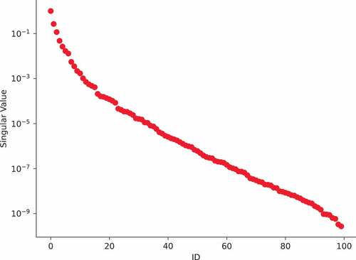Snapshots were generated using the $n_{\mathrm{s}\mathrm{n}\mathrm{a}\mathrm{p}}$ = 100 parameter realizations obtained from a Latin hypercube design. The average wall time to solve the FOM to a 1 × 10⁻⁶ GMRes tolerance on a 2.40-GHz Intel i9-9980HK CPU was 0.126 s. The scalar flux solutions for the snapshots are shown in Fig. 1. The singular values are plotted in Fig. 2.

TABLE I Parameter Distributions for the Slab Benchmark

	Material
Parameter	Source [0, 0.1] $\mathrm{c}\mathrm{m}$	Scatterer (0.1, 0.8) $\cup$ (0.9, 1] $\mathrm{c}\mathrm{m}$	Absorber [0.8, 0.9] $\mathrm{c}\mathrm{m}$
$Q$ ($par$. ${\text{cm}}^{-3}$ . ${\mathrm{s}}^{-1}$)	$\mathcal{U}$ (0, 10)	0	0
${\mathrm{\Sigma }}_t$ (${\text{cm}}^{-1}$)	$\mathcal{U}$ (0, 1)		$\mathcal{U}$ (5, 10)
$c$	$\mathcal{U}$ (0.7, 1)		$\mathcal{U}$ (0.05, 0.1)

Fig. 1. 100 snapshots for the slab benchmark.

Fig. 2. Normalized singular values using 100 snapshots.

In all, 100 new parameter realizations were sampled and used to evaluate the ROM’s performance in terms of accuracy and speedup. The ROM was tested using two angleset configurations. The angle-independent configuration seeks the same expansion coefficients for all 128 discrete directions. The angle-dependent configuration, on the other hand, splits the 128 directions into eight anglesets and allows different expansion coefficients for each angleset. Figures 3 and 4 summarize the ROM error and speedup relative to the FOM. As expected, the ROM error decreases as more POD modes are kept. With 40 modes, the average relative error norms for the angle-independent and angle-dependent cases are 7.21 × 10⁻⁴% and 2.01 × 10⁻⁴%, respectively. If 0.01% error is allowable, only 24 and 18 modes are required in the angle-independent and angle-dependent-cases, respectively. For a given number of modes, the angle-dependent approach is more accurate than the angle-independent approach. This is because the dependent approach allows for the decoupling of anglesets from each other, with local coefficients allowing for a locally optimal solution.

Fig. 3. Relative error norm of the ROM as a function of the number of basis vectors used for the slab benchmark. The boxes show the quartiles of the 100 relative error norms, while the whiskers extend to show the rest of the distribution.

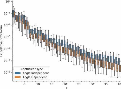
Fig. 4. Speedup of the ROM as a function of the number of basis vectors used for the slab benchmark.

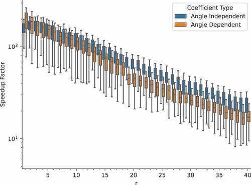
The speedup decreases with the number of modes because the time required to assemble and solve a rank $r$ system increases with $r$. Furthermore, the speedup for the angle-dependent coefficients is lower than that of the angle-independent coefficients because the dependent method solves a rank 8$r$ system to obtain unique coefficients for each of the eight anglesets. While retaining 40 modes, the angle-independent and angle-dependent ROMs only have average speedups of 25.3 and 17.1, respectively. For an error goal around 0.01%, the speedups are 65.3 and 89.4. Because this is a 1-D, one-group benchmark, the FOM solve times are relatively fast, resulting in lower speedups. Much larger speedups are expected for higher dimensional problems; see the next benchmark case in Sec. IV.C. Finally, note that if the FOM were solved to a smaller tolerance than 1 × 10⁻⁶, it would take longer to solve, resulting in a higher ROM speedup.

To assess the accuracy of the ROM’s spatial reconstruction, the pointwise relative error is plotted in Fig. 5 for the 100 parameter realizations in the testing data set. Most of the ROM solutions are within 0.006% of their FOM counterparts. The parameter realization with the largest pointwise relative error (1.7%) has the smallest total cross section in the scattering material (0.002 cm⁻¹) of all the parameter realizations in the testing data set. This parameter value is lower than all but one of the samples used to train the ROM. The corresponding high (compared to the other test cases) pointwise relative error suggests that adding additional training points in this region of the parameter space could improve ROM accuracy.

Fig. 5. ROM pointwise relative error (40-mode angle-dependent ROMs); 100 testing parameter realizations shown. Maximum pointwise error is 1.7%.

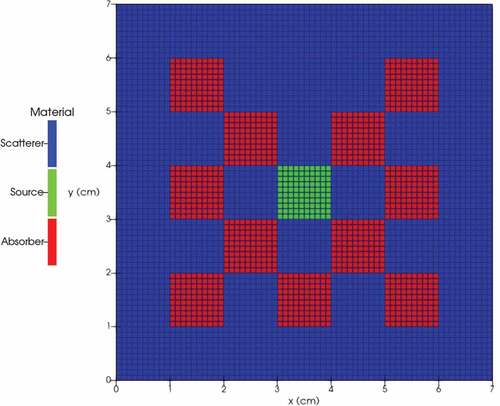
IV.C. Two-Dimensional, One-Group Checkerboard Benchmark

The geometry for this benchmark⁷⁴ consists of a square domain of scattering material with a centered external source. There are squares of absorbing material embedded in the domain. Vacuum boundary conditions are imposed, and the domain is discretized into 4900 square cells with bilinear discontinuous finite elements. The geometry and spatial discretization are illustrated in Fig. 6. A product quadrature was created by combining an 8-direction Gauss-Legendre polar angle quadrature with a 128-direction Gauss-Chebyshev azimuthal angle quadrature for a total of $D=512$ angles. The energy phase space is discretized using $G=1$ energy group, for a total FOM system size of $N\approx 1.00\times {10}^7$.

Fig. 6. Checkerboard benchmark geometry. The source material has the same cross sections as the scattering material.

Five parameters consisting of absorption ${\mathrm{\Sigma }}_a$ and scattering ${\mathrm{\Sigma }}_s$ cross sections, as well as external source strengths $Q$, were selected as input parameters; their distributions are given in Table II. Within this table, a uniform distribution between $a$ and $b>a$ is denoted by $\mathcal{U}(a,b)$. 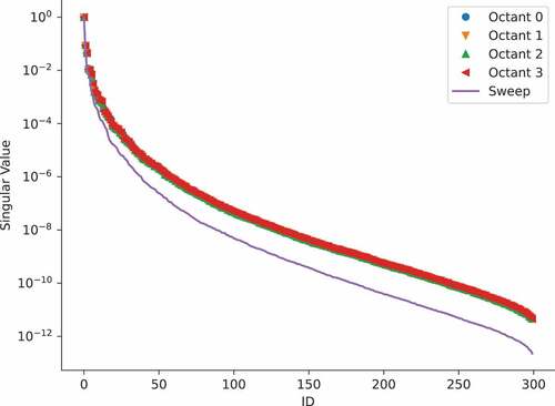Snapshots were generated using the $n_{\mathrm{s}\mathrm{n}\mathrm{a}\mathrm{p}}=300$ (Latin hypercube) parameter realizations from Ref. 61. The average wall time to solve the FOM to a 1 × 10⁻⁶ GMRes tolerance on four 2.20-GHz Intel Xeon Silver 4214 CPUs was 98 s. The scalar flux solutions for three selected snapshots are shown in Fig. 7. Note that because 2-D transport problems are symmetric about the polar angle, only four angular octants need to be solved. Since splitting the last benchmark into eight sets of angle-dependent coefficients yielded more accurate results, a similar approach was utilized for this benchmark. To ease the burden of computing the SVD, the snapshots were split by angular octant and the SVD for each of the four relevant octants was independently computed to yield POD modes for each octant. The standard octants of the unit sphere were utilized. The singular values of each octant’s angular snapshots are plotted in Fig. 8 along with the singular values of the flux moment snapshots used in the sweep-based ROM.

TABLE II Parameter Distributions for the Checkerboard Benchmark

	Material
Parameter	Absorber	Scatterer
${\mathrm{\Sigma }}_a$ (${\mathrm{c}\mathrm{m}}^{-1}$)	$\mathcal{U}$ (7.5, 12.5)	$\mathcal{U}$ (0.0, 0.5)
${\mathrm{\Sigma }}_s$ (${\mathrm{c}\mathrm{m}}^{-1}$)	$\mathcal{U}$ (0.0, 5.0)	$\mathcal{U}$ (0.5, 1.5)
$Q$ ($par$ . ${\mathrm{c}\mathrm{m}}^{-3}$ . ${\mathrm{s}}^{-1}$)	0	$\mathcal{U}$ (0.0, 2.0)

Fig. 7. Full-order solutions for three of the snapshots. Parameter vectors are reported as ${\mathrm{\Sigma }}_a^{\mathbf{a}\mathbf{b}\mathbf{s}\mathbf{o}\mathbf{r}\mathbf{b}\mathbf{e}\mathbf{r}},{\mathrm{\Sigma }}_a^{\mathbf{s}\mathbf{c}\mathbf{a}\mathbf{t}\mathbf{t}\mathbf{e}\mathbf{r}\mathbf{e}\mathbf{r}},{\mathrm{\Sigma }}_s^{\mathbf{a}\mathbf{b}\mathbf{s}\mathbf{o}\mathbf{r}\mathbf{b}\mathbf{e}\mathbf{r}},{\mathrm{\Sigma }}_s^{\mathbf{s}\mathbf{c}\mathbf{a}\mathbf{t}\mathbf{t}\mathbf{e}\mathbf{r}\mathbf{e}\mathbf{r}},\mathrm{a}\mathrm{n}\mathrm{d}{Q}^{\mathbf{s}\mathbf{c}\mathbf{a}\mathbf{t}\mathbf{t}\mathbf{e}\mathbf{r}\mathbf{e}\mathbf{r}}$.

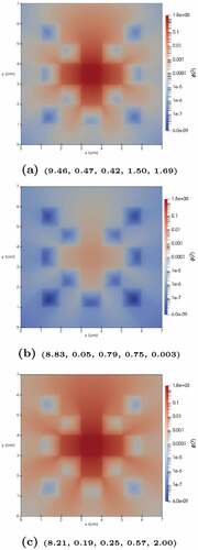
Fig. 8. Normalized singular values of the angular snapshots for each octant of the 300 snapshots, along with the singular values of the flux moment snapshots.

To assess the performance of the ROM, the testing set from Ref. 61 (50 parameter realizations) was used. Figures 9 and 10 summarize the ROM error and speedup relative to the FOM. As expected, the ROM error decreases as more POD modes are kept. The average relative error norms for $r=40$ are 9.04 × 10⁻⁴% and 1.42 × 10⁻⁴%, respectively, for the affine-based and sweep-based ROMs. If 0.01% error is allowable, only 26 and 14 modes are required in the affine and sweep-based ROMs, respectively. For a given value of $r$, the sweep-based ROM has a lower error than the affine-based ROM because the sweep singular values decay faster than the affine singular values. This faster decay allows for a better approximation to the solution with fewer modes. The speedup decreases with the number of modes because the time required to assemble and solve a rank $r$ system increases with $r$. While retaining 40 modes, the affine-based and sweep-based ROMs have average speedups of ~1120 and 0.26, respectively. At the 0.01% error threshold, the speedups are ~4870 and 0.62, respectively.

Fig. 9. Relative error norm of the ROM as a function of the number of basis vectors used for the checkboard benchmark.

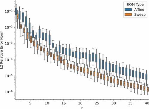
Fig. 10. Speedup of the ROM as a function of the number of basis vectors used for the checkerboard benchmark.

It is evident from these results that the affine-decomposed ROM is significantly more efficient than the sweep-based ROM. Indeed, it actually is faster to solve the FOM than to utilize the sweep-based ROM. Recall that because the moment form of the transport operators is not parametrically affine, the minimally invasive sweep-based ROM must perform $r+1$ full-order transport sweep solves to build the reduced operators for each parameter realization in the online phase. The FOM can solve this problem in fewer than 15 sweeps, thus it is faster than the sweep-based ROM. Even larger speedups are expected for higher dimensional problems such as 3-D multigroup, which we expect to report in a subsequent publication. Finally, note that if the FOM were solved to a smaller tolerance than 1 × 10⁻⁶, it would take longer to solve, resulting in a higher ROM speedup.

To assess the accuracy of the ROM’s spatial reconstruction, the pointwise relative error of the ROM is plotted in Fig. 11 for one of the validation parameter realizations.

Fig. 11. ROM pointwise relative error for one of the 50 validation parameter realizations (affine-decomposed ROM).

IV.D. Two Dimensions, 13 Groups: Graphite Benchmark

The geometry for this benchmark consists of a graphite square with an AmBe neutron source embedded on one side and an array of three BF³ detectors embedded in borated high-density polyethylene (HDPE) on the other. To introduce more variance into the problem, a section of the graphite between the source and the detectors was allowed to have variable density. The entire apparatus is surrounded by air. Vacuum boundary conditions are imposed, and the domain is discretized into 24 636 cells. The geometry is illustrated in Fig. 12. A product quadrature was created by combining a 4-direction Gauss-Legendre polar angle quadrature with a 64-direction Gauss-Chebyshev azimuthal angle quadrature for a total of $D=128$ angles. The energy phase space is discretized using $G=13$ energy groups, for a total FOM system size of $N\approx 1.23\times {10}^8$.

Fig. 12. Graphite benchmark geometry.

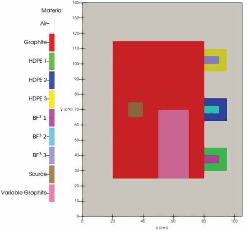
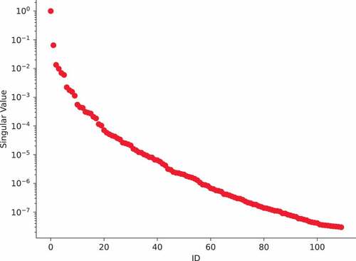
Four parameters were selected. The first three consist of the mass fraction of boron, uniformly distributed between 0% and 7.2% in the HDPE block around each detector. The fourth parameter is the density of the variable graphite section, uniformly distributed between 0 g/cm³ (void, no graphite) and 2.26 g/cm³ (no void, full graphite). Snapshots were generated using $n_{\mathrm{s}\mathrm{n}\mathrm{a}\mathrm{p}}=200$ parameter realizations obtained from a Latin hypercube design. The average wall time to solve the FOM to a 1 × 10⁻⁶ GMRes tolerance on 40 2.20-GHz Intel Xeon Silver 4214 CPUs was 72 s. The scalar flux solutions for groups 9 and 12 of the three selected snapshots are shown in Fig. 13. A single SVD was computed for the agglomeration of all directions and energy groups. The singular values are plotted in Fig. 14.

Fig. 13. Full-order solutions for three of the snapshots. The top and bottom rows correspond to energy groups 9 and 12, respectively, while each column corresponds to a snapshot. Parameter vectors are reported as quadruplets of boron fraction 1, boron fraction 2, boron fraction 3, and variable graphite density.

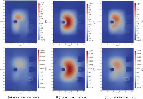
Fig. 14. Normalized singular values of the energy- and direction-agglomerated angular snapshots.

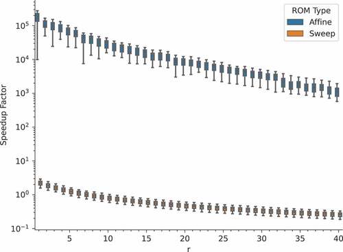
In all, 100 new parameter realizations were sampled and used to evaluate the ROM’s performance in terms of accuracy and speedup. The ROM was tested using three groupset configurations: a monolithic approach in which the same expansion coefficients are applied across all energy groups, a group-dependent approach in which each group has its own coefficients, and a groupset–dependent approach. In the groupset–dependent approach, three groupsets consisting of groups 0 to 6, 7 to 10, and 11 and 12 were chosen based on solution similarity within each set. For simplicity, the monolithic approach was utilized in the angular dimension, where the same expansion coefficients were applied over all directions. Figures 15 and 16 summarize the ROM error and speedup relative to the FOM. As expected, the ROM error decreases as more POD modes are kept. With 60 modes, the average relative error norms for the monolithic, group-dependent, and groupset–dependent cases are 2.1 × 10⁻⁴%, 3.1 × 10⁻⁴%, and 2.2 × 10⁻⁴%, respectively. If 0.01% error is allowable, only 25 modes are required for all coefficient types.

Fig. 15. Relative error norm of the ROM as a function of the number of basis vectors used for the graphite benchmark.

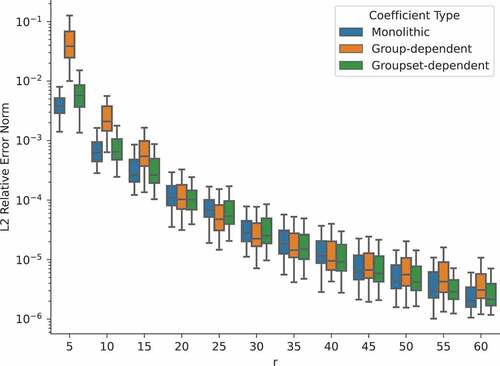
Fig. 16. Speedup of the ROM as a function of the number of basis vectors used for the graphite benchmark.

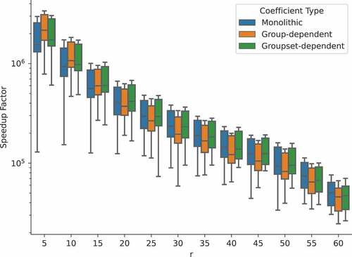
The speedup decreases with the number of modes because the time required to assemble and solve a rank $r$ system increases with $r$. While retaining 60 modes, ROMs have average speedups of 60 200, 52 800, and 54 600 for each coefficient type. For an error goal around 0.01%, the speedups are 370 200, 346 100, and 399 800. Finally, note that if the FOM were solved to a smaller tolerance than 1 × 10⁻⁶, it would take longer to solve, resulting in a higher ROM speedup.

In this benchmark, the detector zones are obvious choices for RoIs. In Fig. 17, we display the RoI relative error norms (Eq. (38(38) $\mathrm{R}\mathrm{o}\mathrm{I}\mathrm{r}\mathrm{e}\mathrm{l}\mathrm{a}\mathrm{t}\mathrm{i}\mathrm{v}\mathrm{e}\mathrm{e}\mathrm{r}\mathrm{r}\mathrm{o}\mathrm{r}\mathrm{n}\mathrm{o}\mathrm{r}\mathrm{m}(\vec{\theta })=\sqrt{\frac{{\sum }_{g=1}^G||{\vec{\mathrm{\Phi }}}_r^g(\vec{\theta })-{\vec{\mathrm{\Phi }}}^g(\vec{\theta })|{|}_{2,{\mathcal{D}}_{RoI}}^2}{{\sum }_{g=1}^G||{\vec{\mathrm{\Phi }}}^g(\vec{\theta })|{|}_{2,{\mathcal{D}}_{RoI}}^2}}=\sqrt{\frac{{\sum }_{g=1}^G{\int }_{RoI}{({\varphi }_r^g(\vec{\theta },\vec{r})-{\varphi }^g(\vec{\theta },\vec{r}))}^{2}dV}{{\sum }_{g=1}^G{\int }_{RoI}{\varphi }^g{(\vec{\theta },\vec{r})}^{2}dV}}.$(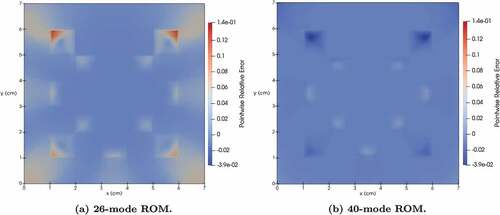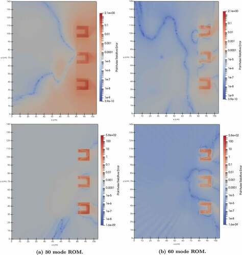38) )) for the central detector (BF³ 2) and the HDPE surrounding it (HDPE 2). For comparison purposes, the ROM relative error over the entire domain (i.e., all materials) is also plotted Fig. 17 for the monolithic ROM. Note that the RoI relative errors in the HDPE and BF³ materials are significantly higher than the full-domain relative error. More information may be gleaned by examining the pointwise relative error of the ROM, plotted in Fig. 18 for one of the validation parameter realizations. These plots show that the pointwise relative error is higher at the RoIs compared to the rest of the domain. This explains the higher than average RoI relative error norms. For results such as these in which the region of highest error occurs in the RoIs, it may be advantageous to utilize a ROM that optimizes the solution in the RoIs instead of over the full domain. We refer the interested reader to Ref. 47 for an example of such a QoI-based ROM.

Fig. 17. RoI relative error norm of the ROM as a function of the number of basis vectors used.

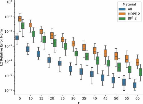
Fig. 18. Pointwise relative error for one of the 100 validation parameter realizations. The top and bottom rows correspond to energy groups 9 and 12, respectively, while each column corresponds to the rank of the ROM.

V. CONCLUSIONS

In this work, we developed a data-driven, projection-based ROM for parametric radiation transport problems that utilize solvers that rely on matrix-free transport sweeps. The FOMs and ROMs are parametric in the sense that they depend on input parameters that can vary, as is often the case in multiquery scenarios such as design optimization and uncertainty quantification. A POD approach was used to learn an appropriate subspace to represent new parameter-dependent transport solutions.

In previous work,⁶¹ the sweep preconditioned form of the transport operator was used to project the transport equation and compute the reduced-order operators. Even though this was minimally invasive to a S_N transport code, the computation of the reduced-order operators had to be repeated for any new parameter realization, making that sweep-based ROM marginally useful.

In this work, we used the affine-decomposition property of the transport operators with respect to the parameters. In doing so, one can isolate parameter-independent portions of the transport equation and thus perform the costly projection step once for all, significantly reducing the online computation of the ROM. In the online phase, the parametric reduced operators are rapidly built in a matrix-free manner by combining the parameter components with their parameter-independent counterparts. The reduced-order system is rapidly solved for the subspace coordinates at which the ROM solution resides.

The affine-based ROM is significantly faster than both the full-order transport solve and the previously devised sweep-based ROM. However, one must be able store large angular flux quantities, such as snapshots and POD modes; in addition, this method is code intrusive in the computation of the parameter-independent components of the projection terms. Therefore, access to the source code is necessary to implement this ROM approach. This affine-based ROM was applied to 1-D, 2-D, and multigroup 2-D transport benchmarks and was found to deliver large speedups over full-order transport solves while retaining solution accuracy. The affine ROM also outperformed the sweep-based ROM in terms of speedup while yielding similar solution accuracy.

The affine-based ROM discussed the concept of angle-sets, allowing each grouping of angles to have a different set of expansion coefficients. Angular splitting is an interesting topic, and its impact is problem dependent. Sensitivity was observed in the 1-D benchmark in that the more anglesets that were used, the lower the ROM error for a given number of modes $r$. The same trend was not observed in subsequent 2-D problems in which the choice of anglesets has little impact on the ROM error. This is a topic that warrants additional research.

Acknowledgments

The authors acknowledge the Texas Advanced Computing Center at The University of Texas at Austin for providing High Performance Computing resources that contributed to the research results reported within this paper (http://www.tacc.utexas.edu).

Disclosure Statement

No potential conflict of interest was reported by the authors.

Additional information

Funding

This work was made possible through a grant by the U.S. Department of Defense, Defense Threat Reduction Agency under award no. HDTRA1-18-1-0020. The content of the information does not necessarily reflect the position or the policy of the federal government, and no official endorsement should be inferred.This material is based on work supported under an Integrated University Program Graduate Fellowship. Any opinions, findings, conclusions or recommendations expressed in this paper are those of the authors and do not necessarily reflect the views of the U.S. Department of Energy, Office of Nuclear Energy.

APPENDIX

Algorithms for computing the parameter-independent portions of the affine decomposition ${\mathit{W}}^T\mathit{T}(\vec{\theta }){\mathit{U}}_r$, ${\mathit{W}}^T\mathit{M}\mathbf{\Sigma }(\vec{\theta })\mathit{D}{\mathit{U}}_r$, and ${\mathit{W}}^T\vec{Q}(\vec{\theta })$

A.I. OFFLINE COMPUTATION OF THE PARAMETER-INDEPENDENT CONTRIBUTION TO ${\mathit{W}}^T\mathit{G}{\mathit{U}}_r$

Algorithm A.1 is used for offline computation of the parameter-independent contribution to ${\mathit{W}}^T\mathit{G}{\mathit{U}}_r:$

Table

Algorithm A.1: Offline computation of parameter-independent contribution to W^TGUr.

Input: W^T, the transposed projection matrix (shape $r\times N_{\mathrm{\Psi }}$)

Input: Ur, the POD modes (shape $N_{\mathrm{\Psi }}\times r$)

Result: Parameter-independent part of W^TGUr is written to file.

file = NewFile();

for d = 1 to D do

for g = 1 to G do

W^TGU = ZeroMatrix(r, r)

for c = 1 to Ncells do

/* Stiffness term */

stiff_c = GetCellStiffness(c)

stiff_c_d = DotProduct(${\vec{\mathrm{\Omega }}}_d$, stiff_c)

u_c = ExtractCellMatrix(Ur, c, d, g)

gu_c = MatVecMult(stiff_c, u_c)

/* Surface terms */

cell_faces = GetCellFaces(c)

for face in cell_faces do

d_dot_n = DotProduct(face.normal, ${\vec{\mathrm{\Omega }}}_d$)

if d_dot_n $\ge$ 0 then

continue / / Skip outgoing faces

end

mass_F = GetCellIncomingSurfaceMass(c, face)

mass_F_dot = d_dot_n * mass_F

u_c_upstream_f = ExtractCellUpstreamMatrix(Ur, c, face, d, g)

u_c_f = ExtractCellMatrix(Ur, c, face, d, g)

gu_c += MatVecMult(mass_F_dot, u_c_upstream_f - u_c_f)

end

w^T_c = ExtractCellMatrix(W^T, c, d, g)

W^TGU += MatMatMult(w^T_c, gu_c)

end

file.Write(d, g, W^TGU)

end

end

file.Close();

A.II. OFFLINE COMPUTATION OF THE PARAMETER-INDEPENDENT CONTRIBUTION TO ${\mathit{W}}^T\mathit{T}\left(\vec{\theta }\right){\mathit{U}}_r$

Algorithm A.2 is used for offline computation of the parameter-independent contribution to ${\mathit{W}}^T\mathit{T}\left(\vec{\theta }\right){\mathit{U}}_r$

Table

Algorithm A.2: Offline computation of parameter-independent contribution to W^TGUr.

Input: W^T, the transposed projection matrix (shape $r\times N_{\mathrm{\Psi }}$)

Input: Ur, the POD modes (shape $N_{\mathrm{\Psi }}\times r$)

Result: Parameter-independent part of W^TGUr is written to file.

file = NewFile();

for k = 1 to Nmat do

for d = 1 to D do

for g = 1 to G do

W^TTU = ZeroMatrix(r, r)

for c in CellsInMaterial(k) do

w^T_c = ExtractCellMatrix(W^T, c, d, g)

u_c = ExtractCellMatrix(Ur, c, d, g)

/* total cross section factored out, to be applied in online

phase */

mass_c = GetCellMass(c)

tu_c = MatVecMult(mass_c, u_c)

W^TTU += MatMatMult(w^T_c, tu_c)

end

file.Write(k, d, g, W^TTU)

end

end

end

file.Close();

A.III. OFFLINE COMPUTATION OF THE PARAMETER-INDEPENDENT CONTRIBUTION TO ${\mathit{W}}^T\mathit{M}\mathbf{\Sigma }(\vec{\theta })\mathit{D}{\mathit{U}}_r$

Algorithm A.3 is used for offline computation of the parameter-independent contribution to ${\mathit{W}}^T\mathit{M}\mathbf{\Sigma }(\vec{\theta })\mathit{D}{\mathit{U}}_r:$

Table

Algorithm A.3: Offline computation of parameter-independent contribution to ${\mathit{W}}^T\mathit{M}\sum (\vec{\theta })\mathit{D}{\mathit{U}}_r$

Input: W^T, the transposed projection matrix (shape $r\times N_{\mathrm{\Psi }}$)

Input: Ur, the POD modes (shape $N_{\mathrm{\Psi }}\times r$)

Result: Parameter-independent part of ${\mathit{W}}^T\mathit{M}\sum (\vec{\theta })\mathit{D}{\mathit{U}}_r$ is written to file.

file = NewFile();

for k = 1 to Nmat do

for d = 1 to D do

for $d\prime$ = 1 to D do

for g = 1 to G do

for $g\prime$ = 1 to G do

for m = 1 to Nmom do

${\mathrm{W}}^{\mathrm{T}}\mathrm{M}\text{diams}\mathrm{D}\mathrm{U}$ = ZeroMatrix(r, r)

for c in CellsInMaterial(k) do

u_c = ExtractCellMatrix(Ur, c, $d\prime$, $g\prime$)

/* D${ }_{d\prime }$ applied for moment m */

du_c = ComputeDirectionContributionToMoment(u_c, $d\prime$, m)

/* scattering moment factored out, applied in online

phase */

mass_c = GetCellMass(c)

$\sigma$du_c = MatVecMult(mass_c, du_c)

m$\sigma$du_c = ApplyMomentToDiscrete($\sigma$du_c, m, d)

w^T_c = ExtractCellMatrix(W^T, c, d, g)

${\mathrm{W}}^{\mathrm{T}}\mathrm{M}\text{diams}\mathrm{D}\mathrm{U}$ += MatMatMult(wT c, m$\sigma$du_c)

end

file.Write(k, d, $d\prime$, g, $g\prime$, m, W^TTU)

end

end

end

end

end

end

file.Close();

A.IV. OFFLINE COMPUTATION OF THE PARAMETER-INDEPENDENT CONTRIBUTION TO ${\mathit{W}}^T\vec{Q}(\vec{\theta })$

Algorithm A.4 is used for offline computation of the parameter-independent contribution to ${\mathit{W}}^T\vec{Q}(\vec{\theta })$:

Table

Algorithm A.4: Offline computation of parameter-independent contribution to ${\mathit{W}}^T\vec{Q}(\vec{\theta })$.

Input: W^T, the transposed projection matrix (shape $r\times N_{\mathrm{\Psi }}$)

Result: Parameter-independent part of ${\mathit{W}}^T\vec{Q}(\vec{\theta })$ is written to file.

file = NewFile();

for k = 1 to Nmat do

for d = 1 to D do

for g = 1 to G do

W^TQ = ZeroVector(r)

for c in CellsInMaterial(k) do

/* source strength factored out, to be applied in online

phase */

load_c = GetCellLoad(c)

w^T_c = ExtractCellMatrix(W^T, c, d, g)

W^TQ += MatVecMult(w^T_c, load_c)

end

file.Write(k, d, g, W^TQ)

end

end

end

file.Close();

References

- M. P. ADAMS et al., “Provably Optimal Parallel Transport Sweeps on Semi-Structured Grids,” J. Comput. Phys., 407, 109234 (2020); https://doi.org/10.1016/j.jcp.2020.109234.
- J. I. VERMAAK et al., “Massively Parallel Transport Sweeps on Meshes with Cyclic Dependencies,” J. Comput. Phys., 425, 109892 (2021); https://doi.org/10.1016/j.jcp.2020.109892.
- M. HANUS and J. C. RAGUSA, “Thermal Upscattering Acceleration Schemes for Parallel Transport Sweeps,” Nucl. Sci. Eng., 194, 10, 873 (2020); https://doi.org/10.1080/00295639.2020.1767436.
- J. S. HESTHAVEN, G. ROZZA, and B. STAMM, Certified Reduced Basis Methods for Parameterized Partial Differential Equations, Springer International Publishing (2016); https://doi.org/10.1007/978-3-319-22470-1.
- Reduced Order Methods for Modeling and Computational Reduction, A. QUARTERONI and G. ROZZA Eds., Springer International Publishing (2014); https://doi.org/10.1007/978-3-319-02090-7.
- Reduced Basis Methods for Partial Differential Equations, A. QUARTERONI, A. MANZONI, and F. NEGRI Eds., Springer International Publishing (2016); https://doi.org/10.1007/978-3-319-15430-2.
- Model Reduction of Parameterized Systems, P. BENNER et al. Eds., Springer International Publishing (2017); https://doi.org/10.1007/978-3-319-58785-1.
- J. J. DUDERSTADT and L. J. HAMILTON, Nuclear Reactor Analysis, John Wiley & Sons, Inc. (1976).
- G. I. BELL and S. GLASSTONE, Nuclear Reactor Theory, Van Nostrand Reinhold Company (1970).
- M. HADIGOL and A. DOOSTAN, “Least Squares Polynomial Chaos Expansion: A Review of Sampling Strategies,” Comput. Methods Appl. Mech. Eng., 332, 382 (2018); https://doi.org/10.1016/j.cma.2017.12.019.
- M. M. R. WILLIAMS, “Polynomial Chaos Functions and Neutron Diffusion,” Nucl. Sci. Eng., 155, 1, 109 (2007); https://doi.org/10.13182/NSE05-73TN.
- M. WILLIAMS, “Polynomial Chaos Functions and Stochastic Differential Equations,” Ann. Nucl. Energy, 33, 9, 774 (2006); https://doi.org/10.1016/j.anucene.2006.04.005.
- M. EATON and M. WILLIAMS, “A Probabilistic Study of the Influence of Parameter Uncertainty on Solutions of the Neutron Transport Equation,” Prog. Nucl. Energy, 52, 6, 580 (2010); https://doi.org/10.1016/j.pnucene.2010.01.002.
- L. GILLI et al., “Performing Uncertainty Analysis of a Nonlinear Point-Kinetics/Lumped Parameters Problem Using Polynomial Chaos Techniques,” Ann. Nucl. Energy, 40, 1, 35 (2012); https://doi.org/10.1016/j.anucene.2011.09.016.
- L. GILLI et al., “Uncertainty Quantification for Criticality Problems Using Non-intrusive and Adaptive Polynomial Chaos Techniques,” Ann. Nucl. Energy, 56, 71 (2013); https://doi.org/10.1016/j.anucene.2013.01.009.
- Z. M. PRINCE and J. C. RAGUSA, “Parametric Uncertainty Quantification Using Proper Generalized Decomposition Applied to Neutron Diffusion,” Int. J. Numer. Methods Eng., 119, 9, 899 (2019); https://doi.org/10.1002/nme.6077.
- J. P. SENECAL and W. JI, “Characterization of the Proper Generalized Decomposition Method for Fixed-Source Diffusion Problems,” Ann. Nucl. Energy, 126, 68 (2019); https://doi.org/10.1016/j.anucene.2018.10.062.
- S. GONZÁLEZ-PINTOR, D. GINESTAR, and G. VERDÚ, “Using Proper Generalized Decomposition to Compute the Dominant Mode of a Nuclear Reactor,” Math. Comput. Modell., 57, 7, 1807 (2013); https://doi.org/10.1016/j.mcm.2011.11.066.
- A. L. ALBERTI and T. S. PALMER, “Reduced-Order Modeling of Nuclear Reactor Kinetics Using Proper Generalized Decomposition,” Nucl. Sci. Eng., 194, 10, 837 (2020); https://doi.org/10.1080/00295639.2020.1758482.
- K. A. DOMINESEY and W. JI, “Reduced-Order Modeling of Neutron Transport Separated in Space and Angle via Proper Generalized Decomposition,” presented at the International Conference on Mathematics Computational Methods Applied to Nuclear Science and Engineering, August 25-29 (2019).
- K. A. DOMINESEY and W. JI, “Reduced-Order Modeling of Neutron Transport Separated in Energy by Proper Generalized Decomposition with Applications to Nuclear Reactor Physics,” J. Comput. Phys., 449, 110744 (2022); https://doi.org/10.1016/j.jcp.2021.110744.
- J. KOU, S. L. CLAINCHE, and W. ZHANG, “A Reduced-Order Model for Compressible Flows with Buffeting Condition Using Higher Order Dynamic Mode Decomposition with a Mode Selection Criterion,” Phys. Fluids, 30, 1, 016103 (2018); https://doi.org/10.1063/1.4999699.
- H. LU and D. M. TARTAKOVSKY, “Lagrangian Dynamic Mode Decomposition for Construction of Reduced-Order Models of Advection-Dominated Phenomena,” J. Comput. Phys., 407, 109229 (2020); https://doi.org/10.1016/j.jcp.2020.109229.
- D. A. BISTRIAN and I. M. NAVON, “Randomized Dynamic Mode Decomposition for Nonintrusive Reduced Order Modelling,” Int. J. Numer. Methods Eng., 112, 1, 3 (2017); https://doi.org/10.1002/nme.5499.
- Z. K. HARDY, J. E. MOREL, and C. AHRENS, “Dynamic Mode Decomposition for Subcritical Metal Systems,” Nucl. Sci. Eng., 193, 11, 1173 (2019); https://doi.org/10.1080/00295639.2019.1609317.
- R. G. MCCLARREN, “Calculating Time Eigenvalues of the Neutron Transport Equation with Dynamic Mode Decomposition,” Nucl. Sci. Eng., 193, 8, 854 (2019); https://doi.org/10.1080/00295639.2018.1565014.
- T. SAYADI et al., “Parametrized Data-Driven Decomposition for Bifurcation Analysis, with Application to Thermo-Acoustically Unstable Systems,” Phys. Fluids, 27, 3, 037102 (2015); https://doi.org/10.1063/1.4913868.
- Q. HUNH, M. TANO, and J. C. RAGUSA, “Parametric Dynamic Mode Decomposition for Reduced Order Modeling,” J. Comput. Phys. (2022, accepted for publication).
- Z. BAI, “Krylov Subspace Techniques for Reduced-Order Modeling of Large-Scale Dynamical Systems,” Appl. Numer. Math., 43, 1, 9 (2002); https://doi.org/10.1016/S0168-9274(02)00116-2.
- Y. YUE and K. MEERBERGEN, “Parametric Model Order Reduction of Damped Mechanical Systems via the Block Arnoldi Process,” Appl. Math. Lett., 26, 6, 643 (2013); https://doi.org/10.1016/j.aml.2013.01.006.
- K. LEE and K. T. CARLBERG, “Model Reduction of Dynamical Systems on Nonlinear Manifolds Using Deep Convolutional Autoencoders,” J. Comput. Phys., 404, 108973 (2020); https://doi.org/10.1016/j.jcp.2019.108973.
- B. A. KHUWAILEH and W. A. METWALLY, “Gaussian Processa Aproach for Dose Mapping in Radiation Fields,” Nucl. Eng. Technol., 52, 8, 1807 (2020); https://doi.org/10.1016/j.net.2020.01.013.
- K. PEARSON, “On Lines and Planes of Closest Fit to Systems of Points in Space,” London, Edinburgh Dublin Philosophical Magazine J. Sci., 2, 11, 559 (1901); https://doi.org/10.1080/14786440109462720.
- D. T. CROMMELIN and A. J. MAJDA, “Strategies for Model Reduction: Comparing Different Optimal Bases,” J. Atmos. Sci., 61, 17, 2206 (Sep. 1, 2004); https://journals.ametsoc.org/view/journals/atsc/61/17/1520-0469_2004_061_2206_sfmrcd_2.0.co_2.xml (current as of Feb. 23,2022).
- I. T. JOLLIFFE and J. CADIMA, “Principal Component Analysis: A Review and Recent Developments,” Philos. Trans. R. Soc. A Math. Phys. Eng. Sci., 374, 2065, 20150202 (2016); https://doi.org/10.1098/rsta.2015.0202.
- C. W. ROWLEY and J. E. MARSDEN, “Reconstruction Equations and the Karhunen–Lo`eve Expansion for Systems with Symmetry,” Physica D, 142, 1, 1 (2000); https://doi.org/10.1016/S0167-2789(00)00042-7.
- P. V. BAYLY et al., “Predicting Patterns of Epicardial Potentials During Ventricular Fibrillation,” IEEE Trans. Biomed. Eng., 42, 9, 898 (1995); https://doi.org/10.1109/10.412656.
- E. KRUEZER and O. KUST, “Analysis of Long Torsional Strings by Proper Orthogonal Decomposition,” Arch. Appl. Math., 67, 68 (1996); https://doi.org/10.1007/BF00787141.
- M. AZEEZ and A. VAKAKIS, “Proper Orthogonal Decomposition (POD) of a Class of Vibroimpact Oscillations,” J. Sound Vib., 240, 5, 859 (2001); https://doi.org/10.1006/jsvi.2000.3264.
- B. EPUREANU, K. HALL, and E. DOWELL, “Reduced-Order Models of Unsteady Viscous Flows in Turbomachinery Using Viscous-Inviscid Coupling,” J. Fluids Struct., 15, 2, 255 (2001); https://doi.org/10.1006/jfls.2000.0334.
- M. RAJAEE, S. K. F. KARLSSON, and L. SIROVICH, “Low-Dimensional Description of Free-Shear-Flow Coherent Structures and Their Dynamical Behavior,” J. Fluid Mech., 258, 1 (1994); https://doi.org/10.1017/S0022112094003228.
- J. BURKARDT, M. GUNZBURGER, and H.-C. LEE, “POD and CVT-based Reduced-Order Modeling of Navier–Stokes Flows,” Comput. Methods Appl. Mech. Eng., 196, 1, 337 (2006); https://doi.org/10.1016/j.cma.2006.04.004.
- F. FANG et al., “A POD Reduced Order Unstructured Mesh Ocean Modelling Method for Moderate Reynolds Number Flows,” Ocean Modell., 28, 1, 127 (2009); https://doi.org/10.1016/j.ocemod.2008.12.006.
- A. BAKHSHINEJAD et al., “Merging Computational Fluid Dynamics and 4D Flow MRI Using Proper Orthogonal Decomposition and Ridge Regression,” J. Biomech., 58, 162 (2017); https://doi.org/10.1016/j.jbiomech.2017.05.004.
- K. K. NAGARAJAN et al., “Open-Loop Control of Cavity Noise Using Proper Orthogonal Decomposition Reduced-Order Model,” Comput. Fluids, 160, 1 (2018); https://doi.org/10.1016/j.compfluid.2017.10.019.
- D. LI et al., “An Efficient Implementation of Aeroelastic Tailoring Based on Efficient Computational Fluid Dynamics-based Reduced Order Model,” J. Fluids Struct., 84, 182 (2019); https://doi.org/10.1016/j.jfluidstructs.2018.10.011.
- T. BUI-THANH et al., “Goal-Oriented, Model-Constrained Optimization for Reduction of Large-Scale Systems,” J. Comput. Phys., 224, 2, 880 (2007); https://doi.org/10.1016/j.jcp.2006.10.026.
- P. GERMAN and J. C. RAGUSA, “Reduced-Order Modeling of Parameterized Multi-Group Diffusion k-Eigenvalue Problems,” Ann. Nucl. Energy, 134, 144 (2019); https://doi.org/10.1016/j.anucene.2019.05.049.
- A. G. BUCHAN et al., “A POD Reduced-Order Model for Eigenvalue Problems with Application to Reactor Physics,” Int. J. Numer. Methods Eng., 95, 12, 1011 (2013); https://doi.org/10.1002/nme.4533.
- A. BUCHAN et al., “A POD Reduced Order Model for Resolving Angular Direction in Neutron/Photon Transport Problems,” J. Comput. Phys., 296, 138 (2015); https://doi.org/10.1016/j.jcp.2015.04.043.
- A. C. HUGHES and A. G. BUCHAN, “A Discontinuous and Adaptive Reduced Order Model for the Angular Discretization of the Boltzmann Transport Equation,” Int. J. Numer. Methods Eng., 121, 24, 5647 (2020); https://doi.org/10.1002/nme.6516.
- J. TENCER et al., “Reduced Order Modeling Applied to the Discrete Ordinates Method for Radiation Heat Transfer in Participating Media,” Proc. Heat Transfer Summer Conf. (Nov. 11, 2016); https://doi.org/10.1115/HT2016-7010.
- J. TENCER et al., “Accelerated Solution of Discrete Ordinates Approximation to the Boltzmann Transport Equation for a Gray Absorbing-Emitting Medium via Model Reduction,” J. Heat Transfer, 139, 12, 122701 (2017); https://doi.org/10.1115/1.4037098.
- I. UDAGEDARA et al., “Reduced Order Modeling for Accelerated Monte Carlo Simulations in Radiation Transport,” Appl. Math. Comput., 267, 237 (2015); https://doi.org/10.1016/j.amc.2015.03.113.
- Y. SUN et al., “A POD Reduced-Order Model for Resolving the Neutron Transport Problems of Nuclear Reactor,” Ann. Nucl. Energy, 149, 107799 (2020); https://doi.org/10.1016/j.anucene.2020.107799.
- A. SARTORI et al., “Comparison of a Modal Method and a Proper Orthogonal Decomposition Approach for Multi-group Time-Dependent Reactor Spatial Kinetics,” Ann. Nucl. Energy, 71, 217 (2014); https://doi.org/10.1016/j.anucene.2014.03.043.
- K. TSUJITA, T. ENDO, and A. YAMAMOTO, “Fast Reproduction of Time-Dependent Diffusion Calculations Using the Reduced Order Model Based on the Proper Orthogonal and Singular Value Decompositions,” J. Nucl. Sci. Technol., 58, 2, 173 (2021); https://doi.org/10.1080/00223131.2020.1814891.
- J. M. COALE, “Reduced Order Models for Thermal Radiative Transfer Problems Based on Low-Order Transport Equations and the Proper Orthogonal Decomposition,” North Carolina State University ProQuest Dissertations Publishing. (2019).
- R. PINNAU, Model Reduction via Proper Orthogonal Decomposition, pp. 95–109, Springer Berlin Heidelberg, Berlin, Heidelberg (2008); https://doi.org/10.1007/978-3-540-78841-65.
- P. A. BEHNE, J. C. RAGUSA, and J. E. MOREL, “Model-Order Reduction Approaches for SN Radiation Transport,” Proceedings, International Conference on Mathematics Computational Methods Applied to Nuclear Science and Engineering, Portland, OR, August 25-29, 2019, (2019).
- P. BEHNE, J. VERMAAK, and J. C. RAGUSA, “Minimally-Invasive Parametric Model-Order Reduction for Sweep-Based Radiation Transport,” J. Comput. Phys., 469 (2022).
- P. BENNER, S. GUGERCIN, and K. WILLCOX, “A Survey of Projection-based Model Reduction Methods for Parametric Dynamical Systems,” SIAM Rev., 57, 4, 483 (2015); https://doi.org/10.1137/130932715.
- C. E. HEANEY et al., “Reduced-Order Modelling Applied to the Multigroup Neutron Diffusion Equation Using a Nonlinear Interpolation Method for Control-Rod Movement,” Energies, 14, 5, 1350 (2021); https://doi.org/10.3390/en14051350.
- P. A. BEHNE, J. C. RAGUSA, and M. TANO, “Projection-based Model Order Reduction Based on Affine Decomposition of the Operators,” Proceedings, International Conference on Mathematics Computational Methods Applied to Nuclear Science and Engineering, October 3-7, 2021 (2021).
- M. TANO et al., “Affine Reduced-Order Model for Radiation Transport Problems in Cylindrical Coordinates,” Ann. Nucl. Energy, 158, 108214 (2021); https://doi.org/10.1016/j.anucene.2021.108214.
- T. BUI-THANH, K. WILLCOX, and O. GHATTAS, “Parametric Reduced-Order Models for Probabilistic Analysis of Unsteady Aerodynamic Applications,” AIAA J., 46, 10, 2520 (2008); https://doi.org/10.2514/1.35850.
- W. R. D. BOYD III, “Reactor Agnostic Multi-Group Cross Section Generation for Fine-Mesh Deterministic Neutron Transport Simulations,” PhD Thesis, Massachusetts Institute of Technology, Department of Nuclear Science and Engineering (2017).
- T. R. HILL, “ONETRAN: A Discrete Ordinates Finite Element Code for the Solution of the One-Dimensional Multigroup Transport Equation,” Los Alamos National Laboratory (1975).
- W. H. REED and T. R. HILL, “Triangular Mesh Methods for the Neutron Transport Equation,” Los Alamos Scientific Laboratory (1973).
- T. A. WAREING et al., “Discontinuous Finite Element SN Methods on Three-Dimensional Unstructured Grids,” Nucl. Sci. Eng., 138, 3, 256 (2001); https://doi.org/10.13182/NSE138-256.
- T. BUI-THANH, K. WILLCOX, and O. GHATTAS, “Model Reduction for Large-Scale Systems with High-Dimensional Parametric Input Space,” SIAM J. Sci. Comput., 30, 6, 3270 (2008); https://doi.org/10.1137/070694855.
- B. PEHERSTORFER and K. WILLCOX, “Data-driven Operator Inference for Nonintrusive Projection-based Model Reduction,” Comput. Methods Appl. Mech. Eng., 306, 196 (2016); https://doi.org/10.1016/j.cma.2016.03.025.
- K. KUNISCH and S. VOLKWEIN, “Optimal Snapshot Location for Computing POD Basis Functions,” ESAIM: Math. Model. Numer. Anal., 44, 3, 509 (2010); https://doi.org/10.1051/m2an/2010011.
- T. A. BRUNNER, “Forms of Approximate Radiation Transport,” Technical report, Sandia National Laboratories (2002).