
 ?Mathematical formulae have been encoded as MathML and are displayed in this HTML version using MathJax in order to improve their display. Uncheck the box to turn MathJax off. This feature requires Javascript. Click on a formula to zoom.
Abstract
In recent years, molten salt reactors (MSRs) have gained new momentum thanks to their potential for innovation in the nuclear industry, and several studies on their compliance with all the expected safety features are currently underway. In terms of passive safety, a strategy currently envisaged in accidental scenarios is to drain by gravity the molten salt, which acts both as fuel and coolant, in an emergency draining tank, ensuring both a subcritical geometry and proper cooling. To activate the draining system, a freeze plug, made of the same salt used in the core, is expected to open when the temperature in the core reaches high values. Up to this point, the freeze valve is still a key concept in the molten salt fast reactor (MSFR), and special attention must be paid to its analysis, given the requirement for passive safety, especially focusing on melting and solidification phenomena related to the molten salt mixture.
This work aims to contribute to the macroscale modeling of melting and solidification phenomena relevant to the analysis of the freeze valve behavior. In particular, the focus is on the identification of the numerical models that can be adopted to achieve the quantitative insights needed for the design of the freeze valve. Among the ones available in the literature, the most appropriate models were selected based on a compromise between accuracy and computational efficiency. A critical look at the models allows for a synthetic and consistent formulation of the numerical models and their implementation in the open-source software OpenFOAM. The code was subsequently verified using analytical and numerical solutions already well established in the literature.
A good agreement between the results produced by the developed solver and the reference solutions was obtained. In the end, the code was applied to simple case studies related to the freeze valve system, focusing on recognizing whether the developed code can model physical phenomena that can occur in a freeze valve. The results of the simulations are encouraging and show that the code can be used to model single-region melting or solidification problems. As such, this work constitutes a starting point for further development of the code, intending to achieve better quantitative predictions for the design of a freeze valve.
I. INTRODUCTION
Generation-IV reactors[Citation1] are nuclear reactor concepts having the potential to bring various benefits to the nuclear industry, including increased safety, reduced proliferation risks, economical affordability, sustainability of the fuel cycle, and management of the waste inventory. Among them, the molten salt fast reactor (MSFR) is the current reference design studied within the Generation-IV International Forum, and its safety barriers are the object of the SAMOSAFER European project.Footnotea A mixture of chloride or fluoride salt containing the dissolved nuclear fuel is pumped and circulated through the primary system, acting as coolant and fuel.[Citation2] In case of an accident, the molten salt is drained by gravity from the core to a casing located below the core, where proper cooling and subcriticality are ensured. The draining system is connected through 16 pipes to the bottom of each one of the external loops.
To enhance the passive safety feature of the reactor, the MSFR design is provided with freeze valves. Such a component was first used in the Molten Salt Reactor Experiment (MSRE) as a way to overcome the difficulty of finding a reliable mechanical valve that could bear the aggressive environment of the system.[Citation3] The freeze valve allows for draining of the molten salt when an accident makes the temperature of the core rise over acceptable levels. In this case, the valve melted by the heat stored in metal plates in contact with it, kept hot by electric resistances. However, as designed in the MSRE, the freeze valve was not a fully passive safety feature.[Citation3] For this reason, novel commitment is necessary to achieve a design that is compliant with the requirement for passive safety. The modern concept of a MSFR envisions the use of a freeze valve as well, positioned vertically in a portion of the draining piping in the proximity of the core. The freeze valve is still considered today as a valuable solution to be implemented in future molten salt reactors (MSRs), not only because of the compatibility of the material in the demanding environment of the core. Especially after the Fukushima Daiichi accident, the concept of passive safety is a fundamental requirement for nuclear reactors, and the ability of the valve to self-modulate its state, using the phase change, in response to temperature variations in the core has frequently been equated to safety function passivity. For this reason, it is fundamental to be able to reach a fully passive design of the freeze valve, and the capability of the valve to open in any accidental scenario, including a loss of outside power, is of great importance.
Melting and solidification of the fuel salt play a key role in the design and safety of the MSFR, such as the design of the freeze plug,[Citation4] the analysis of accident scenarios where the solidification of the salt might be a risk,[Citation5] or the possible formation of a frozen salt film on the reactor vessel walls, protecting them from corrosion.[Citation6] A mathematical description of the melting and solidification problem allows for a quantitative description of a phase-change transient. The most basic mathematical description of melting and solidification phenomena is due to Josef Stefan,[Citation7] and the respective mathematical problem is known as the Classical Stefan Problem. However, this problem does not have exact or approximate analytical solutions for many real engineering situations. For instance, most practical situations are multidimensional in nature, while analytical solutions are only available in one dimension.[Citation8] For this reason, the urge for the development of numerical methods has been present in the scientific literature since at least the late 1980s.
However, the numerical modeling of the phase change is a challenging task due to two main issues. On the one hand, the phase change from liquid to solid is a multiscale process, meaning that the dynamics of the phase change are governed by different physical phenomena that span from the atomic scale to the macroscale.[Citation9] The coupling of these phenomena represents a challenge both to the physical modeling and to the discretization process of the numerical models. On the other hand, with the macroscale approach, two other challenges emerge: (1) the choice of the appropriate values for the thermophysical properties of the solid phase that are required to embed all the complexity of a possibly anisotropic microstructure (as in the case of the eutectic solidification of the FLiNaK) in averaged quantities, such as the thermal conductivity tensor, the equivalent elastic-plastic modulus, the equivalent thermal stress tensor, and possibly others[Citation10]; and (2) the nonlinearity of the macroscale formulation, as the liquid front depends on the temperature of the system, and vice versa.
Historically, the study of phase-change materials (PCMs) has been a big incentive for the development of numerical methods for melting and solidification. Nowadays, the study of PCM using computational fluid dynamics is widespread and has been documented in several papers. (Reference [Citation11] provides a review on the topic.) Typically, there are two main groups of numerical phase-change models: fixed-grid (or physical-grid) and variable-grid (or transformed-grid) models. In the latter, two sets of equations are implemented, one for each phase (solid and liquid). Indeed, the grid is adapted to the interface location, and the two separate domains are coupled using transference terms between the phases.
On the other hand, fixed-grid methods consider a single set of discretized conservation equations, valid both for the solid and the liquid domains. Differently from variable-grid methods, the interface is not tracked explicitly, but is it reconstructed a posteriori after an appropriate field variable. Hence, no run-time modification of the computational domain is required. The energy conservation and the Navier-Stokes equations are modified to properly take into account the two main phenomena that take place during phase change, namely, latent heat and velocity transition, the latter being the momentum exchange between the solid and the liquid phases. The main advantage of the fixed-grid methods is their simplicity, which has determined their rise in popularity, making them a standard approach in the field of the numerical modeling of metallurgical solidification processes and PCMs.[Citation11]
Since in such methods the discontinuity is not treated by separating the computational domain, the interface is “smeared” in a finite length, often called a “mushy zone.” Such a halfway state is determined by the presence of both solid and liquid in different proportions, according to the temperature of the mixture. Indeed, excluding two exceptions, namely, eutectic systems and pure elements, in most solidification systems the phase change from liquid to solid and the relative evolution of latent heat will occur over a temperature range in which both the liquid and solid coexist.[Citation12] For this reason, the fixed-grid methods are conceptually more suitable for nonisothermal phase changes. However, they have been largely adapted for use also for isothermal phase changes, even if in this case the interface between solid and liquid is sharp, by forcing the mushy region to be as localized as possible.
A few preliminary numerical analyses of the freeze plugs already exist, such as in Refs. [Citation4,Citation13–15], and they all make use of fixed-grid numerical methods for the phase change to make quantitative predictions about the melting times and other significant engineering quantities of the valves. In Ref. [Citation13], a high-temperature molten salt test loop was constructed and tested, both numerically and experimentally. The working fluid was FLiNaK salt, while the valve was made of Hastelloy C276 and set into a horizontal position, having the shape of a pipe squashed in the middle portion. The numerical analysis consisted of a steady-state analysis of the thermal behavior, using a Finite Elements (FE) calculation, which was validated by the experimental setup.
In Ref. [Citation14], a freeze valve was built and experimentally studied to investigate which phenomena impacted the melting time of the freeze valve. The study allowed for assessing the fundamental parameters to be considered in the construction of a freeze valve, such as the liquid temperature, the depth, the diameter, and the thermal diffusivity. In Ref. [Citation4], a numerical study was conducted to offer preliminary insights into different engineering solutions and parameters. The salt considered in this case was LiF4, and two possible configurations were investigated: the first was called “single plug,” which was a single cylinder of solid salt, and the other was called “multiple plugs,” in which several cylinders of salt were inserted in a drilled metal plate. In Ref. [Citation15], taking advantage of the knowledge given by experiments and using numerical simulations, useful recommendations and guidelines for the design of a cold plug were provided.
In Ref. [Citation10], a multiscale model for the SWATH-S (an experiment dealing with the solidification of FLiNaK salt) was developed with the aim of taking into account the coupling between the phenomena occurring at the macroscale with those that take place at the mesoscale. The macroscale model was developed using an arbitrary Lagrangian-Eulerian method, where the solid is described by a Lagrangian approach and the liquid by an Eulerian approach. Furthermore, the mesh was adapted to the shrinkage of the solid phase, and a novel thermodynamically consistent derivation of the conservation equations was developed. For what concerns the mesoscale model, it is refined enough to describe the phase segregation in the solid phase thanks to a thermodynamical model conceptually similar to the macroscale one.
If on one hand, models like the latter are precious to estimate the parameters for the macroscale models, they are hardly scalable to large systems due to the intensive computational effort required. The aim of this work is to provide a previously developed OpenFOAM solver for MSFR analysis[Citation16–19] with the capability to model the freeze plug in operational- and safety-related transients. Due to the requirement of modeling the entire MSFR system, the development focus is on the fixed-grid approach with a macroscale phase-change representation [e.g., apparent Heat Capacity (AHC) method[Citation20] and Source Term (ST) method].[Citation21] This way, the solver does not need Lagrangian mesh capabilities and does not depend on complex thermodynamics mesoscale models that can hinder the simulation of a full-scale system.
This paper is organized as follows. A review of the numerical modeling used in the developed code is formalized in Sec. II. Afterward, the code is verified in simple benchmark test cases (Sec. III). Finally, the verified code is used to simulate freeze valve–like scenarios to test and see which phenomena the code can model when dealing with realistic cases (Sec. IV).
II. THEORETICAL FRAMEWORK AND NUMERICAL MODELING
As mentioned previously, the two main physical phenomena that have to be addressed in the numerical modeling for melting and solidification are the latent heat and the velocity transition. From a theoretical perspective, the present work adopts the framework of the Continuum Mixture Theory (CMT)[Citation22] in which each phase constituting the mixture is seen as an individual subsystem, given that the interaction terms with other phases are properly treated, and assuming that the properties of the mixture can be described as mathematical consequences of properties of the constituting phases and that the mean collective mixture behavior is governed by equations similar to those governing the individual component (single-fluid model).
In this framework, a few simplifying assumptions allow for writing the equations for the mass, momentum, and energy conservation in a familiar form, suitable to be solved by the established numerical procedure for coupled elliptic partial differential equations with slight modifications for the specificity of the melting problem. Assumptions invoked in the development of such equations include (1) saturated mixture conditions, (2) laminar, constant viscosity, and Newtonian flow in the liquid phase, (3) thermophysical properties independent from pressure and temperature, meaning constant-phase specific heat capacities ( and
), and constant-phase densities (
and
), except for variations in the buoyancy term for the liquid, (4) validity of the Boussinesq approximation, and (5) local thermodynamic equilibrium. In addition, (6) the solid phase is assumed to be nondeforming and free of internal stress, while (7) the multiphase region is viewed as a porous solid characterized by an isotropic permeability.[Citation22] Moreover, in the present work, (8) the salt is seen as a pure substance, without any subconstituent. This is done for the sake of simplicity, since the objective of the present work is to address the numerical models for the solution of the melting problem. Nonetheless, the CMT allows for taking into account the transport of constituents in a natural way, as can be seen in the pioneering work of Bennon and Incropera.[Citation22]
However, some of these simplifying assumptions might introduce errors for melting and solidification problems, i.e., assumptions (3), (4), and (5) are acceptable if the solid and the liquid are within a small temperature range from the melting temperature, but they can generate large errors when larger temperature variations are considered. The impact of higher-order terms on the dependency of the density from the temperature for the FLiNaK salt has been extensively studied in Ref. [Citation10]. Here it is demonstrated that, while it is true that the impact of the solute-driven convection is important close to the interface, its relevance is limited in the very proximity of the interface. When moving away from the interface, these gradients are rapidly smeared out. On the contrary, the thermal gradients can extend over the whole domain. Hence, the effective influence of solute buoyancy in the velocity field generated in the domain is usually much smaller than that of thermal buoyancy.
To achieve higher accuracy in this aspect of the modeling, future work could include solute-driven convection terms and the second-order terms evaluated in Ref. [Citation10]. Moreover, while assumption (6) is useful in the scope of this work to focus on the numerical modeling of the melting phenomena, a complete analysis of the freeze valve should likely include the modeling of internal stresses in the solid. For instance, Ref. [Citation10] shows that thermal gradients produce thermal stresses close to the interface. Other clusters of thermal stresses might be present close to the walls due to the constraint of the boundary and to the heat flux coming from the cooling system of the valve. Moreover, during melting transients, the thermal stresses produced by the high thermal gradient might induce cracks in the solid. Assumption (7) is largely used in studies of phase-change processes,[Citation11] and it is modeled by a Darcy source term (DST) in the momentum equation. In the case of the FLiNaK salt, the coefficient of this source term can be calculated by mesoscale models, as in Ref. [Citation10]. With these assumptions, the conservation equations of the system are
where
| = | mixture velocity | |
| = | mixture temperature | |
| = | mixture pressure | |
| = | mixture density | |
| = | mixture-specific enthalpy | |
| = | mixture thermal conductivity | |
| = | density of the liquid phase | |
| = | viscosity of the liquid phase. |
The term present in EquationEq. (2)
(2)
(2) models the exchange terms between the solid and liquid, and the choice of its physical and numerical modeling is called velocity transition modeling (VTM). The momentum source term
depends on the volume liquid fraction
(not to be confused with the gravity force
), and the liquid fraction depends on the temperature, so that the momentum and the energy equations are coupled.
is any heat source that may be added according to the specific case.
In the energy equation, the specific enthalpy depends on the temperature
, and a closure relation must be defined to close the system. Together with the choice of the closure equation, the numerical modeling of the energy equation is called latent heat modeling (LHM).
II.A. Latent Heat Modeling
Analytically, latent heat is modeled through the Stefan condition,[Citation8] which states that the latent heat released due to the interface displacement equals the net amount of heat delivered to or from the interface itself per unit area per unit time:
where is the specific latent heat,
is the velocity of the interface,
is the heat flux, and
is the normal to the interface.
However, this condition does not represent how fixed-grid methods deal with LHM because they do not track explicitly the position of the interface, but the condition must be imposed implicitly directly in the energy equation. In fact, in the framework of CMT, we can define average thermodynamic quantities on a certain volume so that the presence of each phase can be deduced from the mean quantities, such as the mean volumetric enthalpy .[Citation21] The most relevant definitions used in this work are
where
| = | density | |
| = | specific enthalpy of the mixture | |
| = | volume liquid fraction | |
| = | mass liquid fraction | |
| = | a constant offset value, which can be seen as the specific enthalpy of the solid at the melting temperature |
The thermophysical properties are considered independent from the temperature and different from solid to liquid, i.e., and
. This is not a common choice in literature; usually, the thermophysical properties, especially density, are taken to be equal from solid to liquid (as in Refs. [Citation11,Citation21,Citation23–25], including the built-in option proposed in OpenFOAM[Citation26]). CMT on the other hand allows for naturally taking into account different thermophysical properties, which can allow for greater accuracy in the simulations, being a model closer to the physical reality. The vast majority of real substances do not have constant thermophysical properties across the phase transition. Assuming
and
independent from the temperature in a range close to the melting temperature, the average specific enthalpy
can be written as
The choice of considering the specific heat capacity independent from the temperature is valid at the first order only in the proximity of the melting temperature. This was done for the sake of simplicity, even if future work could easily modify the numerical methods proposed in the present work to take into account the dependence of the temperature on the heat capacity.
Combining EquationEqs. (5)(5)
(5) , Equation(6)
(6)
(6) , and Equation(9)
(9)
(9) , and using the fact that
and
, the volumetric enthalpy results in
This quantity allows for writing the energy conservation equation in a simpler way. The energy conservation equation in a pure conduction situation reads
For a system undergoing a phase change, we can write using the notions from CMT. It is noteworthy that, if we decide to express the volumetric enthalpy
as a function of the temperature
, the whole LHM is embedded in the time partial derivative term. Expanding the left side of EquationEq. (11)
(11)
(11) ,
where and
are defined as
Latent heat models differ from one another by the different approaches used to deal with the source terms. In general, the energy equation can be discretized, linearized, and numerically solved for the temperature (temperature-based models), the volumetric enthalpy
, or the specific enthalpy
(enthalpy-based model). Since
depends on
, EquationEq. (11)
(11)
(11) is nonlinear.
Temperature-based latent heat methods introduce a closure relation to couple the two quantities and linearize the problem in . Adopting the general notation proposed in Ref. [Citation12], the discretized form of EquationEq. (11)
(11)
(11) is
where
| = | matrix coefficients for the temperatures | |
| = | linear coefficients for the transient term multiplying the difference of total volumetric enthalpy for cell | |
| = | algebraic source term. |
It is worth noting that even if the starting point was the conduction equation, EquationEq. (15)(15)
(15) is the general discretized form of the energy equation. The convective term and any source term, once linearized in the temperature, can fit in this algebraic form of the temperature equation. Moreover, as it will be later presented in Sec. II.D, the velocity of the solid phase is assumed to be always equal to zero. This allows for simplifying the form of the convection term so that only the enthalpy of the liquid phase is convected. Since
depends on
and temperature-based methods linearize the problem in T and solve the discretized equation in
, this closure relation is adopted as
The different -based methods differ based only on the formulation of the source terms and the coupling algorithm between
and
. On the other hand, in
-based latent heat methods, the discretized energy equation will have a different formulation to accommodate the algebraic solution for enthalpy. In this work, only temperature-based methods were considered due to better compatibility with the current multiphysics solvers previously developed,[Citation16,Citation17] in which the energy equation is solved in temperature. For this reason, two classic temperature-based methods have been implemented, namely, the AHC method and the ST method, along with a novel hybrid method. In the following section, the relationship between
and
is illustrated (closure relation). Afterward, the numerical models of latent heat are presented.
II.B. Closure Relations
All -based latent heat methods are characterized by an energy equation with two coupled variables,
and
(
-based source term). These coupled variables introduce a nonlinearity into the equation, therefore closure equations are needed to link the two of them. Usually, it is assumed that locally the system lies on the
-
curve of the solid-liquid system. This is a simplifying assumption, since in general melting and solidification can be subjected to nonequilibrium phenomena, but the use of an equilibrium curve has the advantage of establishing a bijective relationship between the two quantities of interest, so that deriving one will automatically allow for establishing the other. Moreover, even under the assumption of equilibrium, enthalpy
depends also on other thermodynamical variables.
In the molten salt used in the MSR, there are different species, and their varying concentrations might affect melting and solidification. The modeling of the species concentration is beyond the scope of this work, and the salt will be considered a eutectic mixture that can be described only by the melting temperature and latent heat
. For such isothermal-phase transitions, as a first approximation, one can consider a linear increase of enthalpy with temperature in the pure phases, with a jump discontinuity at the melting temperature. However, from the numerical point of view, introducing such a strong discontinuity poses stability issues, and therefore the phase change is smeared out into a finite interval of temperature. The discontinuity in the enthalpy field is now a weak constraint, as the enthalpy function is now continuous in temperature (with only its derivative discontinuous). This temperature interval is centered on the melting temperature Tm and is called a mushy zone. The variation of the enthalpy with temperature depends on the specific material, and the relations are based on semi-empirical models; once
and
are determined, all other quantities can be retrieved.
In the context of the MSFR, the mushy zone is not physical for what concerns isothermal transition. Therefore, the objective is to make this zone as small as possible, but large enough to have a well-behaved numerical solution. In this case, to mimic the presence of a small nonisothermal-phase transition, one can define a fictitious temperature of solidus and liquidus
that are just a small distance
away from the melting temperature, for instance by setting
and
. The present work considered three simple closure relations; all three of them have a similar impact on the accuracy and stability of the solution, which is the desired outcome since they are just numerical tricks that must tend to the jump discontinuity in
-
. The first relation is a linear
-
relation (), defined as the following, where
is a small temperature interval:
for
Fig. 1. Example of volume fraction and temperature
closure relationship. The liquid fraction is 0 in the solid and 1 in the liquid. In the interval dT, the so-called mushy zone, the liquid fraction varies linearly between 0 and 1.
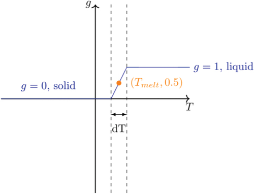
An optimal value of was found to be in the interval [0.1: 10 K]. The second relation is a variation of the previous one, using a sigmoid function centered in Tm for the variation of
, such that
when
and
at
and
, respectively.
The last closure relation that was tested was a linear -
relation. The linear relation
-
automatically sets
to be a quadratic function of
in the mushy zone. To instead impose a linear relationship between
and
, the following is defined:
where the subscript pc stands for phase change. Given the fictitious solidus and liquidus temperatures to be and
, respectively, the corresponding volumetric enthalpies are
Therefore,
II.C. Temperature-Based Models
II.C.1. Apparent Heat Capacity
The AHCs are the most straightforward way to implement latent heat in the heat equation. AHCs make use of the chain rule to approximate the total enthalpy time derivative:
Assuming the relation between and
in time (for instance assuming thermal equilibrium) is known, the derivative
can be evaluated at the previous time step, while the time partial derivative
can be evaluated with the backward Euler method:
The algorithm runs as follows:
At the beginning of the time
The derivative
The energy equation is solved for the field
The calculation for the time
In this method, no iteration is needed to solve the nonlinearity between and
. The coefficients in EquationEq. (16)
(16)
(16) are
The AHC methods are easy to implement and fast running. However, the main drawback is that in some conditions, they could lead to an erroneous “skip” of the latent heat peak, which means that if the temperature has skipped from to
, or vice versa, the mushy zone is avoided. This drawback is usually overcome with the iterative ST at the expense of a higher computational cost.
II.C.2. Source Term Method
The ST is an iterative method that makes use of an inner loop for each time step. In addition to the classical outer loop for time discretization that it is used to solve for the quantities at time (as in the AHC method), an inner loop is used to solve for the nonlinearity between the temperature
and the volume fraction
. To do so, an iteration is carried out between the energy equation (that solves for
) and a formula for the update of the volume liquid fraction
to a new value
, which depends on the value of
calculated by solving the energy equation. Once the convergence for
and
is achieved for the inner loop, the other thermal quantities that depend on
and
are updated and we move to the new time step.
To use the ST, we need to calculate the temperature by solving the energy equation as a function of the liquid fraction
. Hence, the volumetric enthalpy
(and more specifically, its partial time derivative) must be expressed as a function of the liquid volume fraction
and the temperature
, as in EquationEq. (12)
(12)
(12) . Discretizing this latter relation and considering a slow variation of
and of
with time, we get
Here, since both g and T are present at the same time in the equation, we write
to indicate that this quantity will be updated as a function of the temperature
in the inner loop. To obtain consistency between the two fields the following algorithm is used:
At the beginning of the time
The energy equation is solved for the field
The liquid fraction is updated with the following formula:
which is a proposed extension of the formula commonly used for constant thermophysical properties (e.g., in Ref. [Citation26]), extended for different thermophysical properties between the solid and liquid phases.
The liquid fraction is limited between 0 and 1: if
Check if convergence on the fields
If at step 5 both
As can be seen from the formulation of the algorithm, steps 2 to 5 can be considered an inner phase-change loop.
The ST in general is accurate and does not suffer from the problem of latent heat peak skipping, unlike the AHC method. On the other hand, it is much slower than the AHC method, being iterative and slowly converging. To combine the advantages of both methods, a hybrid approach is proposed in the next paragraph. In fact, we exploit the fact that in this formulation of the ST, we can reduce EquationEq. (24)(24)
(24) to the more generic formulation of EquationEq. (16)
(16)
(16) , where the coefficient
corresponds to all the terms multiplying
, becoming an addend to the diagonal of the matrix of the discretized energy equation, while all other terms go under
. This fact allows for easily writing a generic form of the T-based energy equation valid both for the AHC method and ST method, so that an algorithm that can allow for switching at run time from one method to the other just by changing the evaluation of
and
.
II.C.3. Hybrid Method
A novel T-based approach to the LHM is proposed, which is called the “hybrid approach” because it brings together the two existing T-based latent heat models (i.e., the AHC method and the ST method), exploiting the complementary strengths and weaknesses of the two, thus increasing computational efficiency and robustness. On the one hand, the fact that the temperature-based discretized energy equation has the same form independently of the latent heat model used allowed for the implementation of only one T-based solver. In fact, by choosing the appropriate coefficients and
in EquationEq. (16)
(16)
(16) and a closure relationship, one can select and even modify the latent heat model at run time. This was found to be particularly convenient to combine the strengths of the two models in a single hybrid model, reducing their inconveniences. The hybrid model can be presented in the following way:
Start the time-step calculation as the AHC model until the solution of the energy equation.
After the solution of the energy equation, check whether the new temperature field has “skipped” the latent heat peak, i.e., whether in any cell the temperature has skipped from
If the latent heat peak has been skipped, the temperature field is taken back to the value that it had before the solution of the energy equation, i.e., to the value of the beginning of the time step.
If the latent heat peak has been skipped, the latent heat model is changed to the ST one, iterating between the energy equation and the closure relation in the phase-change loop until convergence.
Go to the next time and start the algorithm again.
The combination of the two algorithms allows for exploiting the speed of the AHC method, using it until it fails to include the latent heat peak, in which case the ST method is used to achieve better robustness, using the increased stability with the iterations of the phase-change loop. This was found to be a good compromise between robustness and speed.
II.D. Velocity Transition Modeling
The other main phenomenon in melting and solidification processes is the VTM. As the solid and the liquid phases respond differently to imposed shear stresses, the velocity field must consider this discrepancy. In practice, fixed-grid methods do not implement explicitly the mechanical aspects of the interactions between phases; instead, they modify the classical Navier-Stokes equations for the liquid phase by setting the velocity field equal to a constant in the solid domain, neglecting all mechanical aspects of the system.[Citation11] An additional simplification will be assumed, i.e., the solid phase is considered to be still, so that only the liquid phase is allowed to displace, and the velocity in the solid phase must be equal to zero.
The most popular method for VTM is the DST method, which adds a source term in the Navier-Stokes equations that vastly exceeds the values of all other terms in the equation for the cells in the solid domain, thus forcing the velocity to be zero, while approaching zero in the liquid domain:
where is the Darcy constant and
is the kinematic viscosity. This method allows for a smooth transition of the velocity from solid to liquid with minimum implementation effort.
To solve for the velocity and the pressure field, we make a simplifying assumption to justify the use of the incompressible Navier-Stokes equations. In particular, on one hand, we leverage the work of Ref. [Citation10] in which the impact of higher-order terms on the dependency of the density from the temperature and solute concentration has been studied. It has been demonstrated that the solenoidal condition for the liquid velocity field is appropriate for context in which the temperature of the salt is up to 40 K above the eutectic, while it is true that the impact of the solute-driven convection is important very close to the interface. Moreover, one extra argument that can be used to relax a bit the domain of applicability of the incompressible approximation is the quasi-static nature of the fluid dynamics with respect to the melting dynamics; this justifies the use of
for each fluid dynamical time step. In the present work, we do not take into account the chemical composition of the salt and the modeling of the solute concentrations. If a more precise description of the buoyancy terms is needed in the future, one can consider implementing higher-order terms.
In conclusion, the pressure and velocity field are solved by means of the classical methods used for the Navier-Stokes equations, which are coupled to the energy equation by the DST. The effects of natural convection are modeled through the Boussinesq approximation.
III. MODEL VERIFICATION
As mentioned in Sec. II, the solvers implemented in OpenFOAM are meant to deal with both conductive and convective problems, with the possibility of choosing one of the latent heat models proposed, i.e., AHC method, ST method, or the developed hybrid one (). In this light, the three latter modeling options are tested against two verification cases: a pure conductive one-dimensional (1-D) slab case and a conductive-convection two-dimensional (2-D) square case.
TABLE I OpenFOAM Solvers Implemented
III.A. Conduction Case
Verification of the conduction solvers was carried out by comparing the results with the analytical solution of the two-phase Stefan problem, as suggested in Ref. [Citation8]. The most basic mathematical description of melting and solidification phenomena is due to Josef Stefan,[Citation27] and the respective mathematical problem is indeed known as the Classical Stefan Problem.[Citation7] The unknowns of this problem are the temperature field and the position of the interface between solid and liquid. One of the most interesting aspects of the problem is its nonlinearity, meaning that the position of the interface depends on the temperature, and vice versa. Such a nonlinearity is further complicated by the fact that a condition enforcing an “energy conservative” heat flux must be put on the interface in order to keep into account the latent heat exchanged between solid and liquid.
The Stefan problem has an analytical solution only in a 1-D configuration; it is the melting of a semi-infinite slab , initially solid at temperature
, by imposing a constant temperature
on the face
, with all thermophysical parameters constant. Mathematically, the problem requires finding a temperature distribution
and an interface position function
. The mathematical details are already well known in the literature, and a complete explanation of the problem can be found in Ref. [Citation8].
The conduction solver was verified using the Stefan problem, considering a finite slab, initially solid at a temperature , heated from one side by imposing a fixed temperature
, while the other is adiabatic. Being that Neumann’s solution is valid only for a semi-infinite slab, the numerical solution will accumulate an amount of difference compared to the analytical solution as the time increases. However, for instants at which the heat flux of the analytical solution at
is still sufficiently small, the difference between the analytical and the numerical solution is negligible and will depend only on the accuracy of the numerical method.
III.A.1. Case 1: ;
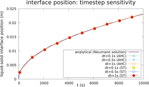
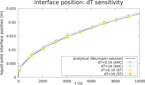
Case 1 is depicted in , whereas the parameters of the case are given in . The AHC method and ST method are compared against the analytical solution of the temperature at t = 1000 s in with remarkably good agreement. A good agreement between the numerical and analytical solution is reached, both for the temperature field and the interface position, as seen in and . The solution is shown to be consistent for different meshes () and time steps (). In addition, the choice of the algorithm for the latent heat model does not influence meaningfully the accuracy of the solution if convergence is achieved and if a correct time step and width of the mushy zone are chosen to ensure energy conservation.
TABLE II Case 1 Parameters
Fig. 2. Depiction of case 1.
Fig. 3. Temperature field at time t = 1000 s (mesh = 100 cells).
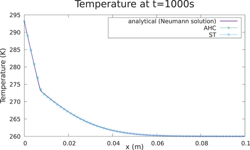
Fig. 4. Mesh sensitivity for the 1-D case (time step = .1 s).
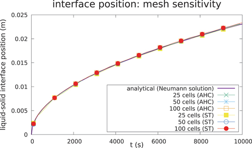
Fig. 5. Sensitivity to different time steps for the 1-D case (mesh = 25 cells).
However, it can be seen that the AHC can suffer a loss of accuracy for some values of the numerical parameter dT, in particular in this case when dT <1 K (), since dT for isothermal transitions is not a physical parameter, and hence its value is not easy to choose a priori before launching a calculation. This effect is even greater for calculations with higher thermal flux, as is shown in the next case.
Fig. 6. Sensitivity to the parameter dT of the latent heat models for the 1-D case (mesh = 25 cells, dT = 0.5 s). It can be seen that the AHC model suffers a loss of accuracy for dT < 1 K.
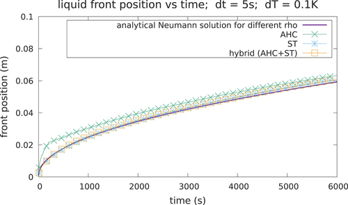
III.A.2. Case 2: ;
Case 2 is depicted in , whereas the parameters of the case are given in . In this case, the properties of the materials are equal to the LiF4 salt, which is used in nuclear applications and has different solid and liquid densities. For this configuration, the choice of the LHM and its numerical parameters will highlight the characteristics of each of these methods; using a mushy zone interval of 0.1 K, the AHC brings to a latent heat peak skipping (), and the agreement with the analytical solution is compromised for the beginning of the transient (where the gradient is steeper), leading to a shift in the numerical solution. On the contrary, the ST is consistently close to the analytical solution. As the latter is an iterative method, convergence was considered achieved when the L2 residual norm of both the and
fields were below 10–5.
TABLE III Case 2 Parameters
Fig. 7. Depiction of case 2.
Fig. 8. Interface position for case 2. With a mushy zone of 0.1 K, the AHC can fail to take into account the latent heat if the is too small, while the ST and hybrid methods guarantee better agreement with the analytical solution.
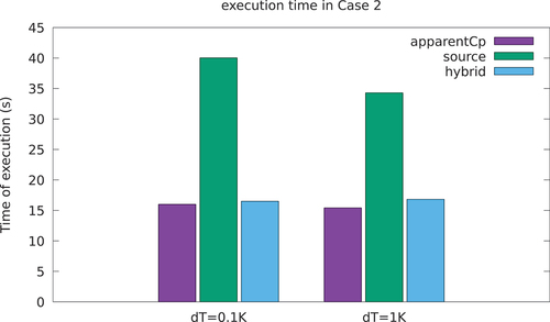
The outcome is that the ST leads to more accurate results at a much slower cost since, on average, around 20 iterations per time step were required for convergence. The dynamic choice of the latent heat model with the hybrid algorithm (AHC + ST) can avoid inaccurate results as it changes the LHM to the ST for all those times in which the peak skip happens with the AHC. With this approach, a good agreement with the reference solution was achieved, with an execution speed comparable to the AHC. The execution times are compared in .
Fig. 9. Execution times for the two cases: for a small computational cost, the hybrid AHC + ST can improve precision (serial execution on desktop PC with Intel(R) CoreTM i7-6700HQ CPU at 2.60 GHz, 4 GB DDR4 RAM).
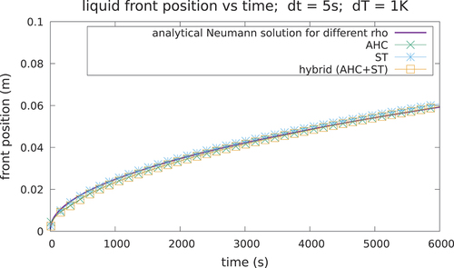
An accurate solution can be obtained also with the AHC by fine-tuning the choice of the width of the mushy zone. With a mushy zone of dT = 1 K, a good agreement with the solution can be obtained (). However, selecting an appropriate value for the dimension of the mushy zone can be tricky, especially using the AHC, since there are no prior considerations that can be made to be sure that the result will take into account the latent heat. On the contrary, the hybrid approach is much less sensitive to the choice of the mushy zone width, while ensuring a good compromise between solution accuracy and speed. The code has been verified also in a 2-D square geometry, obtaining similar results
Fig. 10. Interface position for case 2 with a mushy zone of 1 K. All three models are in good agreement, as the use of a larger helps stabilize the AHC. However, the bigger the
, the farther the case is from an ideal isothermal transition.
III.B. Convection Case
For verification of the convective solver, the numerical solution found in Ref. [Citation25] was used as a reference. The case consists of a cavity of tin, initially solid at , heated from one side by setting the temperature of the left wall at
(). The cavity is a square with a side equal to 0.1 m. The mesh is an orthogonal 100 × 100 cell in the x- and y-directions, with a 7× grading in the x-direction (). As the layer of liquid keeps growing from left to right, the convective motion created by buoyancy becomes stronger and stronger, influencing the shape of the melting front. The resulting flow pattern is laminar and multicellular in nature (i.e., has a structure formed by multiple laminar eddies).
Fig. 11. Verification case for the convection solver. The temperature left wall of the 2-D cavity is set to a value greater than the melting temperature. The emerging flow pattern is an effect of buoyancy.[Citation25]
![Fig. 11. Verification case for the convection solver. The temperature left wall of the 2-D cavity is set to a value greater than the melting temperature. The emerging flow pattern is an effect of buoyancy.[Citation25]](/cms/asset/27a94616-9f44-48bf-8dcd-3fb823f09b8e/unse_a_2229576_f0011_b.gif)
Fig. 12. Computational grid of the 2-D buoyancy-based case consisting in a 100 × 100 mesh with a 7× grading in the x-direction.

The material properties are the ones from Ref. [Citation25]. The hot wall is set at a temperature 3°C greater than the initial solid temperature, which is at a temperature lower than the melting temperature to accommodate the existence of the mushy zone; the chosen mushy zone is 0.1°C thick and the initial temperature of the solid cavity is set to be 0.05°C under the melting temperature ( K,
K, and
K). The numerical schemes used are second-order accurate, and the pressure velocity coupling is solved using the Pressure-Implicit with Splitting of Operators (PISO) algorithm.
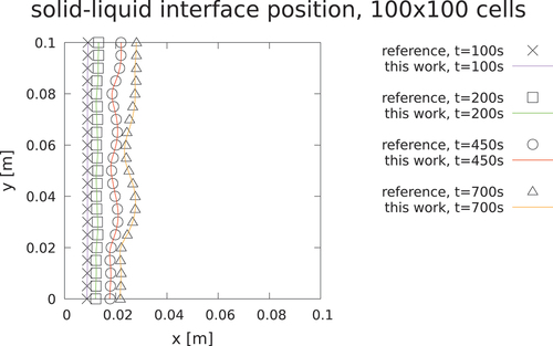
The case couples both the convective part and the conduction, which is relevant for the MSFR case (). The reference solution was obtained using an enthalpy source latent heat model, which is an interesting comparison since the convection solver developed in the present work is temperature based. It can be seen that the source method is a little more in line with the reference solution (). On the other hand, the AHC is slightly underestimating the interface position, while being faster. With such a small temperature gradient, the AHC does not have problems with peak skipping, so the hybrid approach is equivalent to the AHC.
Fig. 13. Buoyancy-induced multicellular pattern develops in the melted zone (t = 450 s; black is solid).
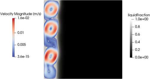
Fig. 14. Position of interface with respect to the reference solution.
IV. APPLICATION TO MOLTEN SALT FREEZE VALVES
As mentioned in Sec. I, one of the main reasons for MSR analysis to model melting and solidification phenomena is the study of the freeze plug. The freeze valve will be essentially a section of a draining pipe with salt in it. In its closed state, a solidified salt prevents the fuel salt from draining, while in the open state, the melting of the freeze plug allows for the discharge of the fuel salt into an emergency tank. The general idea is that in normal conditions, a portion of the draining pipe is cooled to guarantee a closed state of the valve. On the contrary, given an accident scenario, the rise in temperature in the core (and the interruption of the valve cooling) should initiate a melting in the frozen valve, eventually leading to the opening of the valve.
In the MSFR, the exact mechanisms of the opening of the valve are still to be investigated and optimized. On the one hand, if the configuration of the valve is such that, after a certain degree of melting, the hydrostatic pressure is enough to mechanically push the solid plug out of its position and allow for the flow of the liquid, then the opening condition should be investigated in the framework of a thermo-fluid-mechanical analysis. On the other hand, if the configuration of the valve does not provide for a mechanical displacement of the plug, melting will be the dominating phenomenon for the opening of the valve. In the first case, the analysis should focus on the melting of the salt near the wall and how much it affects the mechanical resistance of the valve. In the second case, the shape of the solid-liquid interface, and hence, the heat transfer, will probably be the main factor regulating the dynamic of the valve. The latter was considered in the present study.
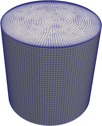
A simple trial configuration was chosen to test the code in a case with conditions that are as close as possible to a real system. The chosen geometry was a simple cylinder, representing the section of the draining pipe occupied by the valve ().[Citation15] The boundary conditions were selected knowing that the position of the valve in the reactor should be at the bottom of each heat exchanger leg. This implies that in nominal working conditions, the temperature at the top face of the valve is around 650°C, while the sides are cooled to a temperature lower than the melting temperature. The subcooling of the valve is one of the key parameters influencing the melting time; in the present work, it was assumed to be 5°C, so with the melting temperature being 568°C, the temperature imposed on the side walls of the valve was 563°C (when the cooling was active). The numerical simulations used a mesh () formed by 120 400 hexahedral elements, with boundary layer refinement on the side wall to account for the steep gradients in this region.
Fig. 15. Dimensions of the section of the pipe considered in the analysis.
Fig. 16. Three-dimensional mesh for the plug.
According to the accident scenario and mechanism activation of the freeze plug, the boundary conditions may change. Two different transient scenarios were modeled. In the first case, the cooling of the valve was switched off (for instance, during a power outage), making the side walls of the valve adiabatic. Considering the recommendations in Ref. [Citation4], a value of 1000°C was imposed at the top face to consider the maximum temperature that builds up during either a loss of heat sink (LOHS) or a loss of fuel accident.
In the second case, a more complex boundary condition was taken into account. As can be seen in Ref. [Citation4], at least when only pure conduction is considered, the melting of the plug can be very slow (longer than 1000 s). A possible solution to the problem is to add a conductive material attached to the wall of the draining pipes, so that it can conduct heat much more rapidly on the side wall of the plug, making it easier to melt close to the walls and eventually helping the displacement of the plug. Modeling such a multicomponent system requires a multiregion approach.
Given the single-region nature of the developed code, a case that mirrors the presence of a metal mass around the tube has been set up through appropriate boundary conditions and a 1-D approach by considering a semi-infinite slab of metal surrounding the plug, starting from the upper surface of the valve and going downward. This slab is initially at T = 563°C. At , the upper surface of the valve and of the metal rise to 1000°C. Due to axial conduction, the metal slab heats up progressively, imposing a temperature boundary condition on the salt cylinder, which is a function of the axial coordinate and of time and coincides with the solution of the heat conduction equation for a semi-infinite slab stated as follows:
The last part of EquationEq. (27)(27)
(27) is the boundary condition imposed on the side wall of the cylinder if the z-axis starts at the upper face of the valve and is directed downward. In all cases, the lower wall of the valve was taken as adiabatic. The cases with the temperature boundary conditions are summarized in .
TABLE IV Temperature Boundary Conditions for the Three Case Studies of the MSFR Freeze Valve
All three cases were considered using both the solver for pure conduction and the one included also for convection. The former represented the most conservative approach, neglecting all movements of the liquid phase. In the latter case, the valve was positioned close enough to the reactor to be affected by the influence of salt circulation. This can be significant, for instance, in a LOHS scenario in which the pump keeps working, and hence salt circulation in the core is still present, or in cases in which the design of the reactor is such that it allows for natural circulation, also in the case of a loss-of-offsite power scenario.
As will be shown, forced convection had a huge impact both on the shape of the melting interface and on the melting time. As a first approximation of the forced convection induced by the motion of the salt in the primary system, the top wall was set to a moving wall with constant velocity along the x-axis equal to 0.1 m/s, which is compatible with the maximum velocity in the core (between 1 to 5 m/s), assuming a velocity one order of magnitude lower due to the proximity of the walls. In addition to forced convection, the contribution of natural circulation also was considered, but its influence turned out to be completely negligible. This means that, for what concerns the geometry used in the present study, natural circulation inside the valve did not have any significant impact.
IV.A. Steady-State Results
Steady-state simulations were performed as the first step to investigate the presence of a stationary solution with the boundary conditions defined in . This kind of simulation can be used to asses if a design complies with the requirement of having a closed valve during normal operations.
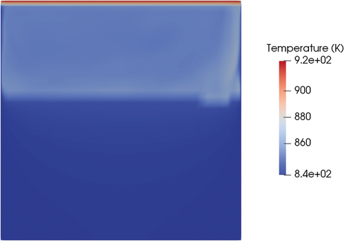
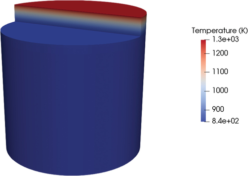
A first simulation was performed with the only-conductive solver. In this case, the position of the interface location () adapted to the shape of the temperature field that developed in the valve (). The valve could be considered closed since the solid plug impeded the flow of the upper liquid to the lower face.
Fig. 17. Section at the midplane of the valve; liquid fraction position at steady state for pure conduction.
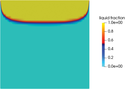
Fig. 18. Temperature field at steady state (conduction).
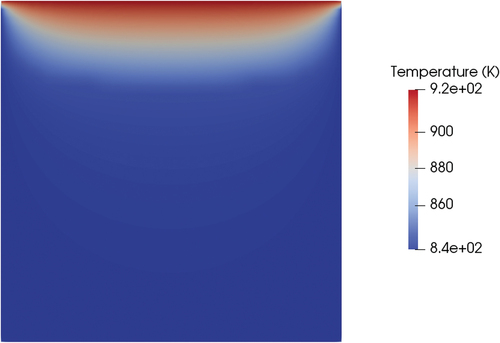
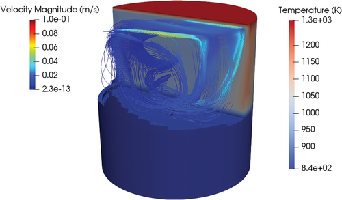
The same case was performed with the meltingPimpleFoam solver (see ) using the hybrid approach as a latent heat model. Setting a velocity on the top wall equal to 0.1 m/s, a stationary solution in the laminar regime did not exist. However, even if the flow pattern is oscillatory, since the melting dynamics is much slower than the fluid dynamics, the solid-liquid interface is on average stable in the same position at around 700 s of physical time. Including the effects of forced convection, the shape of the melting front changed compared to the case of pure conduction (). While the position of the melting front at the centerline of the cylinder was similar (0.14 m for conduction and 0.12 for convection starting from the bottom face), the thickness of the melting front near the wall was much thinner in the case of forced convection, and the same held for the total liquid fraction on the valve (0.21 for conduction and 0.38 for convection). This result proves that, if the valve will rely on mechanical working principles, the thickness of the solid near the walls will be an important parameter to assess the mechanical resistance of the valve and its capability of holding the hydrostatic pressure of the reactor salt. The reason for the difference in the melting front shape is that the convection of energy evens out the temperature field in all the liquid regions ().
Fig. 19. Section at the midplane of the valve; liquid fraction position at steady state with convection (white is solid and blue is liquid) and visualization of the velocity field in the liquid.
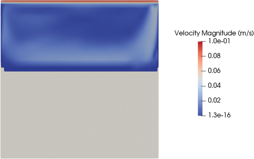
Fig. 20. Temperature field at steady state (convection).
IV.B. Transient Results
The time-dependent analysis was aimed at calculating the time required by the freeze plug to melt and then drain the fuel salt. The initial condition was retrieved from the stationary solution presented in the previous section. At time t = 0, the temperature of the top face of the wall was brought to 1000°C, while the cooling on the sides of the valve was switched off.
First, the case with the adiabatic walls is considered. The evolution of the melting front in the case of pure conduction had a very simple behavior in terms of shape. After the first few tens of seconds, the U-shaped front of the steady state was flattened to a straight shape in which the front proceeded parallel to the top surface. The time of melting for this transient in pure conduction was beyond 10 000 s. This time was way beyond any acceptable limit for the activation of the draining in the reactor core, and this result is in agreement with previous works on freeze valves that suggested that for their use in a passive way with the decay heat from the core to melt the valve, some systems that aid the heat transfer will be required ().[Citation4]
Fig. 21. Temperature field (K) and melting interface in pure conduction (500 s) and adiabatic walls.
Considering also the convection of the fluid, the melting time changed dramatically (). The much more efficient heat transfer in this case led to a much more even temperature profile in the liquid, reducing stratification. This translated to a huge difference in the melting time since for the forced convection case, the first portion of the liquid reached the bottom surface in 920 s, one order of magnitude faster compared to the conduction case. However, this time likely will be too high to guarantee good use of the passive draining system, as it is quite close to the upper recommended limit of 1000 s.[Citation4] Still, this result proved that in the case of LOHS both in the core and in the valve, convection, when present, plays a dominant role in the melting time, and as a consequence, in the opening of the valve.
Fig. 22. Temperature field (K) and melting interface with convection (500 s) and adiabatic walls. The streamline pattern is visualized.
The same transient was performed considering some more realistic boundary conditions with a variable temperature on the side wall (). These conditions mimicked a mass of metal (Hastelloy, ) surrounding the valve and conducting heat from the upper part of the valve (close to the reactor, at 1000°C) to the lower part. A similar configuration can be found in Ref. [Citation4] in which the valve was positioned in a metal tube heated from above. As for the previous transient, the case was initialized starting from the steady-state solution, both for conduction and convection.
TABLE V Thermal Properties of the Hastelloy
For pure conduction, a peculiar shape of the melting front was produced for both the pure conductive and the convective cases ( and , respectively). With the side wall progressively heating, the temperature in the salt near the wall rose faster than the central part of the plug. This created a layer of the melted area that made the solid detach from the side wall. In a configuration of the valve in which the opening is determined by the mechanical resistance of the adhesion of the solid plug to the wall, the speed at which the melted layer is formed is crucial to the estimation of the time of opening of the valve.
Fig. 23. Interface for the conduction case at 600 s (midplane) and variable temperature on the side wall (red is liquid and blue is solid).
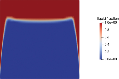
Fig. 24. Interface for the convection case at 600 s (midplane) and variable temperature on the side wall.
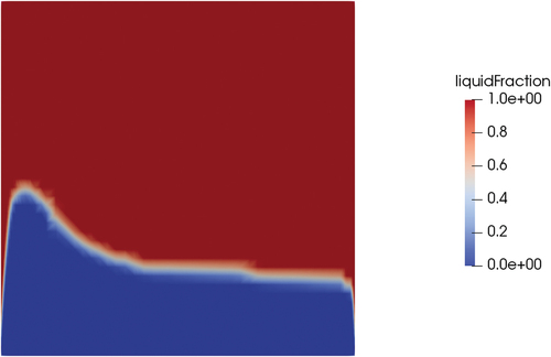
Adding convection, both the shape of the melting front and the melting times were dramatically different from those of the case of pure conduction. The shape of the melting front was influenced by the “erosion” caused by the enhanced heat transfer due to convection ( and ).
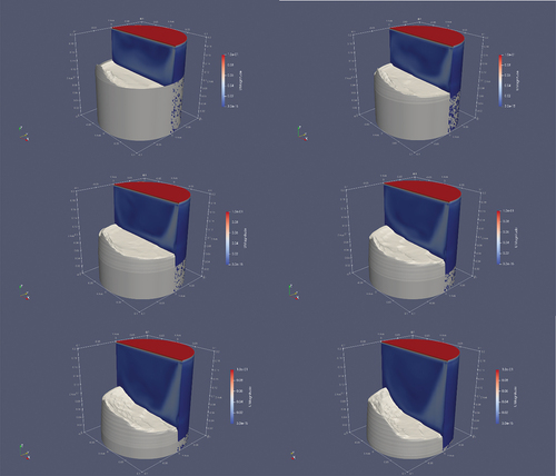
Fig. 25. Shape of the solid plug in time, where deforming is due to the effects of convection. On the right side, the velocity magnitude profile can be seen. The velocity of the upper wall is fixed at 0.1 m/s in the x-direction. On the left side, in white, is the shape of the solid salt. The images shown in this figure are taken at t = 100 s (top left), 200 s (top right), 300 s (center left), 400 s (center right), 500 s (bottom left), and 600 s (bottom right).
A mesh sensitivity analysis was also performed on transient 2 to test the influence of the computational grid on the results. Two additional meshes were adopted, i.e., the first one was obtained by refining the mesh only in the z-direction (doubling the cells) and the second with a refinement in all directions, leading to an increase by a factor 8 of the number of cells with respect to the reference mesh. The results are summarized in the plotting position of the interface at 600 s for the different cases ().
Fig. 26. Shape of the solid-liquid interface at 600 s and at the midplane for the different mesh refinements (in green is the mesh presented in , in blue is the 2× refinement, and in purple is the 8× refinement).
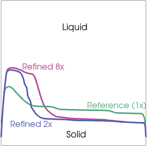
There was an evident impact on the mesh resolution in the zone where the convection was responsible for the melting phenomena, i.e., in the center of the cavity where the motion of the fluid promoted the melting. The increased resolution of the eddies given by the use of a finer mesh led to a different evolution of the fluid motion in the cavity that, integrated along the transient, caused a different position at the interface after 600 s. This difference was more evident when comparing the reference mesh and the refined ×2 with respect to the difference between the two refined meshes, indicating an approach toward mesh independence. On the other hand, such differences had a minor impact on the melting time, which was mainly caused by the heat transfer through the wall conduction.
V. CONCLUSION
This paper aims to provide a previously developed OpenFOAM solver with the capability to model solid-liquid phase-change phenomena in light of the safety analysis of the MSFR and the study of freeze plugs as safety components. The modeling effort was focused on a fixed-grid, temperature-based approach to be compliant with the requirements asked for a reactor-scale representation. To this aim, two well-known algorithms were implemented, namely, the AHC and the ST, along with a novel hybrid method that allows for overcoming some disadvantages in terms of accuracy and computational time. Based on this, a pure conduction and a coupled-conduction-convection solver were developed, the latter being developed with VTM.
The results of the preliminary simulations allowed for drawing some conclusions, both about the developed code and about the freeze valve. For what concerns the developed code, after a verification effort, both pure conduction and convection solvers were demonstrated to be suitable for the simulation of a freeze valve. The choice between the two solvers depended on the configuration of the freeze plug system and the kind of transient. For instance, if the safety analysis involved a LOHS accident with the forced convection of the liquid salt in the primary system, the use of a convective solver was preferable, especially if the valve was located close to the primary circuit. On the other hand, if the movement of the liquid was negligible, the conduction solver could help reduce the computational effort.
As for the design of the freeze valve, the outcomes underline that the freeze valve cannot act as a passive safety system in conditions of adiabatic walls since the time to melt the valve during a transient is well beyond acceptable limits, especially in pure conduction, but also considering the convective contribution. This calls for a solution that involves the melting of the freeze plug not from the top of the system but from the sides, as proposed by other works.[Citation4,Citation10,Citation15]
In terms of future development, given the relevance of the structural components surrounding the freeze plug, the development of a multiregion solver capable of dealing with the different components (valve, metal walls, etc.) of the freeze plug system is of remarkable importance. In terms of boundary conditions, the influence of the primary circuit should be carefully considered, both during nominal operations and during accident scenarios. Even if in this work reasonable boundary conditions were selected, the evolution of the accident transient should be considered directly, implementing the algorithm proposed inside a multiphysics reactor-scale simulation tool. In this way, it will be possible to have a tool that can help in the design and optimization of the freeze plug both in terms of location and performance.
Acronyms
| 1-D | = | = one-dimensional |
| 2-D | = | = two-dimensional |
| AHC | = | = Apparent Heat Capacity Method |
| CMT | = | = Continuum Mixture Theory |
| DST | = | = Darcy Source Term |
| LHM | = | = Latent Heat Modeling |
| LOHS | = | = loss of heat sink |
| MSFR | = | = molten salt fast reactor |
| MSR | = | = molten salt reactor |
| MSRE | = | = Molten Salt Reactor Experiment |
| PCM | = | = phase-change materials |
| ST | = | = Source Term method |
| VTM | = | = Velocity Transition Modeling |
Nomenclature
| = | coefficient of the neighbors of the control volume “p” in the discretized energy equation | |
| = | coefficient of the control volume “p” in the discretized energy equation | |
| = | coefficient of the source term in the discretized energy equation | |
| = | Darcy source term’s constant | |
| = | weighted average of the solid and liquid specific heat capacities | |
| = | specific heat capacity of the liquid | |
| = | specific heat capacity of the solid | |
| dT = | = | temperature difference between the solidus and the liquidus |
| = | momentum exchange source term | |
| = | liquid mass fraction | |
| = | liquid volume fraction | |
| = | gravity acceleration | |
| = | volumetric enthalpy of the mixture | |
| = | average volumetric enthalpy over the control volume “p” | |
| = | specific enthalpy of the mixture | |
| = | specific enthalpy of the liquid | |
| = | specific enthalpy of the solid at the melting temperature | |
| = | specific enthalpy of the solid | |
| = | thermal conductivity | |
| = | latent heat | |
| = | normal to the solid-liquid interface | |
| = | liquid’s kinematic pressure | |
| = | energy source term | |
| = | heat flux | |
| = | linearization coefficient for | |
| = | linearization coefficient for | |
| T = | = | temperature |
| = | melting temperature | |
| = | velocity field, velocity | |
| = | velocity of the solid-liquid interface |
Greek
| = | half of | |
| = | weighted average of the solid and liquid densities | |
| = | density of the liquid | |
| = | density of the solid | |
| = | weighted average heat capacity | |
| = | kinematic viscosity of the liquid |
Research Data
The data that support the findings of this study are openly available in Zenodo at this address: http://doi.org/10.5281/zenodo.7555514.
Disclaimer
The content of this paper does not reflect the official opinion of the European Union. Responsibility for the information and/or views expressed therein lies entirely with the authors.
Disclosure Statement
No potential conflict of interest was reported by the authors.
Additional information
Funding
Notes
a See https://samosafer.eu/.
References
- “Generation IV International Forum 2016 Annual Report,” Generation IV International Forum (2016).
- D. GERARDIN et al., “Design Evolutions of Molten Salt Fast Reactor,” presented at the Int. Conf. on Fast Reactors and Related Fuel Cycles: Next Generation Nuclear Systems for Sustainable Development, June 26. Yekaterinburg, Russia (2017).
- B. M. CHISHOLM, S. L. KRAHN, and A. G. SOWDER, “A Unique Molten Salt Reactor Feature—The Freeze Valve System: Design, Operating Experience, and Reliability,” Nucl. Eng. Des., 368, 110803 (2020); https://doi.org/10.1016/j.nucengdes.2020.110803.
- M. TIBERGA et al., “Preliminary Investigation on the Melting Behavior of a Freeze-Valve for the Molten Salt Fast Reactor,” Ann. Nucl. Energy, 132, 544 (2019); https://doi.org/10.1016/j.anucene.2019.06.039.
- V. VOULGAROPOULOS et al., “Transient Freezing of Water Between Two Parallel Plates: A Combined Experimental and Modelling Study,” Int. J. Heat Mass Trans., 153, 119596 (2020); https://doi.org/10.1016/j.ijheatmasstransfer.2020.119596.
- G. CARTLAND GLOVER, “On the Numerical Modelling of Frozen Walls in a Molten Salt Fast Reactor,” Nucl. Eng. Des., 365, 110290 (2019); https://doi.org/10.1016/j.nucengdes.2019.110290.
- S. C. GUPTA, The Classical Stefan Problem: Basic Concepts, Modelling, and Analysis, No. V. 45 in North-Holland Series in Applied Mathematics and Mechanics, Elsevier (2003).
- V. ALEXIADES and A. D. SOLOMON, Mathematical Modelling of Melting and Freezing Processes, Hemisphere Publishing Corporation (1993).
- A. ONUKI, Phase Transition Dynamics, Cambridge University Press (2002).
- M. TANO RETAMALES, “Development of Multi-Physical Multi-Scale Models for Molten Salts at High Temperature and Their Experimental Validation,” PhD Thesis, University of Grenoble Alpes, LPSC - Laboratoire de Physique Subatomique et de Cosmologie (2018).
- J. H. NAZZI EHMS et al., “Fixed Grid Numerical Models for Solidification and Melting of Phase Change Materials (PCMs),” Appl. Sci., 9, 20, 4334 (2019); https://doi.org/10.3390/app9204334.
- C. R. SWAMINATHAN and V. R. VOLLER, “A General Enthalpy Method for Modeling Solidification Processes,” Metall. Trans. B, 23, 5, 651 (1992); https://doi.org/10.1007/BF02649725.
- Q. LI et al., “Preliminary Study of the Use of Freeze-Valves for a Passive Shutdown System in Molten Salt Reactors,” presented at the ASME/NRC 2014 12th Valves, Pumps, and Inservice Testing Symp., Rockville, Maryland, American Society of Mechanical Engineers (2014).
- I. K. AJI et al., “An Experimental Study on Freeze Valve Performance in a Molten Salt,” Volume 9: Student Paper Competition, American Society of Mechanical Engineers, London, England (2018).
- V. GIRAUD et al., “Development of a Cold Plug Valve with Fluoride Salt,” EPJ Nucl. Sci. Technol., 5, 9, 9 (2019); https://doi.org/10.1051/epjn/2019005.
- E. CERVI et al., “Development of a Multiphysics Model for the Study of Fuel Compressibility Effects in the Molten Salt Fast Reactor,” Chem. Eng. Sci., 193, 379 (2018); https://doi.org/10.1016/j.ces.2018.09.025.
- E. CERVI et al., “Multiphysics Analysis of the MSFR Helium Bubbling System: A Comparison Between Neutron Diffusion, SP3 Neutron Transport and Monte Carlo Approaches,” Ann. Nucl. Energy, 132, 227 (2019); https://doi.org/10.1016/j.anucene.2019.04.029.
- E. CERVI et al., “Development of an SP3 Neutron Transport Solver for the Analysis of the Molten Salt Fast Reactor,” Nucl. Eng. Des., 346, 209 (2019); https://doi.org/10.1016/j.nucengdes.2019.03.001.
- F. CARUGGI et al., “Multiphysics Modelling of Gaseous Fission Products in the Molten Salt Fast Reactor,” Nucl. Eng. Des., 392, 111762 (2022); https://doi.org/10.1016/j.nucengdes.2022.111762.
- C. BONACINA et al., “Numerical Solution of Phase-Change Problems,” Int. J. Heat Mass Trans., 16, 10, 1825 (1973); https://doi.org/10.1016/0017-9310(73)90202-0.
- A. D. BRENT, V. R. ROLLER, and K. J. REID, “Enthalpy-Porosity Technique for Modelling Convection-Diffusion Phase Change: Application to the Melting of a Pure Metal,” Numer. Heat Transfer, 13, 3, 297 (1988); https://doi.org/10.1080/10407788808913615.
- W. BENNON and F. INCROPERA, “A Continuum Model for Momentum, Heat and Species Transport in Binary Solid-Liquid Phase Change Systems—I. and II,” Int. J. Heat Mass Trans., 30, 10, 2161 (1987); https://doi.org/10.1016/0017-9310(87)90094-9.
- R. VISWANATH and Y. JALURIA, “A Comparison of Different Solution Methodologies for Melting and Solidification Problems in Enclosures,” Numer. Heat Transfer Part B, 24, 1, 77 (1993); https://doi.org/10.1080/10407799308955883.
- V. R. VOLLER and C. R. SWAMINATHAN, “General Source-Based Method for Solidification Phase Change,” Numer. Heat Transfer Part B, 19, 2, 175 (1991); https://doi.org/10.1080/10407799108944962.
- N. HANNOUN, V. ALEXIADES, and T. Z. MAI, “A Reference Solution for Phase Change with Convection,” Int. J. Numer. Method, 48, 11, 1283 (2005); https://doi.org/10.1002/fld.979.
- M. TORABI RAD, Solidification Melting Source: A Built-in fvOption in OpenFOAM® for Simulating Isothermal Solidification, Springer International Publishing (2019); https://doi.org/10.1007/978-3-319-60846-4_32.
- J. STEFAN, “Über einige Probleme der Theorie der Wärmeleitung,” Sitzungber. Wien, Akad. Mat. Natur, 98, 473 (1889).