Demographic models of the reproductive process: Past, interlude, and future

Abstract

After 30 years of active development, mechanistic models of the reproductive process nearly stopped attracting scholarly interest in the early 1980s. In the following decades, fertility research continued to thrive, relying on solid descriptive work and detailed analysis of micro-level data. The absence of systematic modelling efforts, however, has also made the field more fragmented, with empirical research, theory building, and forecasting advancing along largely disconnected channels. In this paper we outline some of the drivers of this process, from the popularization of user-friendly statistical software to the limitations of early family building models. We then describe a series of developments in computational modelling and statistical computing that can contribute to the emergence of a new generation of mechanistic models. Finally, we introduce a concrete example of this new kind of model, and show how they can be used to formulate and test theories coherently and make informed projections.

Keywords:

• fertility
• reproductive process
• computational modelling
• approximate Bayesian computation
• agent-based modelling
• microsimulation
• mechanistic modelling

Pioneer models of the family building process

It is almost a century since Corrado Gini introduced the notion of ‘fecundability’, the first major breakthrough that paved the way for the development of models of the reproductive process, defined as the sequence of births a woman experiences and the timing of these events. Gini defined fecundability as the probability that a married woman becomes pregnant in a one-month period, in the absence of contraception (Gini 1924). This idea allowed Gini to investigate physiological variations in fecundity across populations empirically and to propose a simple model of first conceptions.

The first models of the entire reproductive process, however, did not appear until 30 years later, when Louis Henry introduced the concept of ‘natural fertility’. Henry defined this notion as the ‘fertility of a human population that makes no deliberate effort to limit births’ (Henry 1953, p. 135). The idea of natural fertility was not strictly necessary to formulate a family building model, which in its simplest form can be characterized by two parameters: the length of the non-susceptible period and fecundability. But this concept provided an empirical reference, that is, a real-life process against which the results of a model could be assessed, and its parameters estimated.

Henry’s work and that of Dandekar (1955) initiated the first wave of mathematical models of the reproductive process. The substantive aim of these models was to understand the variation in fertility levels across populations that was driven by physiological factors. At the technical level, the main challenge consisted of making tractable but realistic assumptions, for example allowing for heterogeneity or age dependency of parameters such as fecundability. This line of research was developed in the 1950s and 1960s by a community of researchers who drew from an array of mathematical techniques, notably stochastic process theory (Brass 1958; Singh 1963; Perrin and Sheps 1964; Potter and Sakoda 1966; Henry 1972; Sheps et al. 1973; Singh et al. 1974).

The models that came out of this first period provided major insights into the dynamics of the reproductive process and the mechanisms that explained most of the variation in birth rates. But even the most sophisticated mathematical models implied a high degree of abstraction from the real process and often failed to provide a satisfactory fit to the observed data.

The need to study the family building process under less restrictive assumptions led to the emergence of the first computational models (computer models, as they were called at the time). From the 1960s to the 1980s, a number of these models were developed using two alternative approaches: macro- and microsimulation.

Macrosimulation models were also known as ‘expected value’ models because they derived a system of equations linking the distribution of a set of proximate determinants (e.g. duration of postpartum infecundability) to the expected values of fertility outcomes. The system of equations was then solved using numerical methods (Potter 1972; Bongaarts 1977). This approach provided greater flexibility than previous models, making it easier for researchers to handle heterogeneity and age dependency.

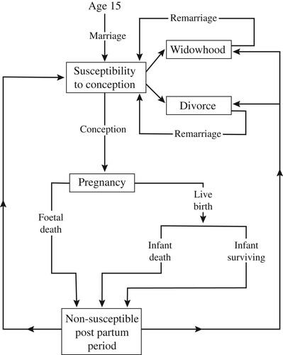
Microsimulation models instead used Monte Carlo techniques in order to draw realizations of individual reproductive trajectories (e.g. Ridley and Sheps 1966; Barrett 1969, 1971; Venkatacharya 1971). Both macro- and microsimulation approaches were algorithmic in nature, using structures such as while loops and if … else statements to define how women move from one state of the reproductive process to another. But microsimulation models, fully expressed in the language of algorithms rather than still relying partly on an equation-based approach, were more flexible: they could be used to formulate an even more realistic representation of the family building process. For example, REPSIM, the model developed by Ridley and Sheps (1966), included a subroutine for the formation and dissolution of unions on top of the typical sequence of states included in earlier models (Figure 1).

Figure 1 Basic operation of the REPSIM model

Source: Developed by Ridley and Sheps (1966).

One obvious aspect of the demographic experience of the past three centuries is that human populations have moved from a natural to a regulated fertility regime, a transition driven by the sustained increase in the use and effectiveness of contraceptive techniques. The reproductive process has become increasingly governed by individual preferences and decisions, rather than by biological factors or socially imposed cultural determinants, such as age at marriage or duration of breastfeeding.

In this context, the notion of desired family size plays a key role. In practice, however, the adaptation of models to the study of regulated fertility did not lead to a significant shift in the focus of analysis. Instead of modelling its determinants and evolution through time, researchers usually drew desired family size from an empirical distribution, and attention remained focused on the proximate determinants of fertility. In other words, the added flexibility and complexity of the available models were used not to provide a qualitatively different type of analysis, but to generate a more nuanced version of the results that had previously been achieved.

Interlude: The rise of statistical demography

The 1966 paper describing REPSIM was cited 34 times after 1990, with merely five citations in demographic journals or working paper series. The book Mathematical Models of Conception and Birth (Sheps et al. 1973) received about 160 citations after 1990, the majority in biostatistics papers, followed by reviews. To place these 160 citations in perspective, Van de Kaa’s paper on ‘Europe’s second demographic transition’ has been cited over 3,000 times (Van de Kaa 1987). It is particularly striking that the notion of fecundability, originally a demographic one, is now most extensively studied in the field of reproductive epidemiology, where major insights have been gained into the individual-level determinants of the waiting time to conception for couples attempting to have a child (Colombo et al. 2000; Dunson et al. 2002; Ecochard 2006).

While it is clear that the research tradition described in the previous section still influences related disciplines, it is equally clear that by the early 1990s it was no longer central in demographic research. This disappearance of family building models—which by contrast with reproductive epidemiology approaches aimed to understand full reproductive histories—was driven by multiple factors. Among factors external to the field, the most important appears to have been the increasing availability of survey and census microdata, which, combined with new statistical methods and the spread of user-friendly software implementing these methods, radically changed the structure of incentives in academic research (Coale and Trussell 1996; Burch 2018). The use of multivariate survival analysis techniques became widespread. Xie (2000) described the influence of the groundbreaking work of Cox (1972) in demography as representing ‘a shift in methodological orientation toward statistical demography […] with attention paid primarily to group differences or the effects of covariates’ (Xie 2000, p. 671). From a career development point of view, ‘empirical’ work relying on general-purpose statistical tools became a more secure investment than model building.

However, the distinction between so-called empirical work and model building is subtler than it might initially appear. Any work that involves a model—whether computational or statistical—cannot be characterized as purely empirical. Statistical models are also theoretical, meaning that they are highly stylized abstractions of a data-generating process. Conversely, computational models can be applied to conduct empirical research. For instance, such models can be used to predict the value of a quantity that exists in the real world (e.g. the number of live births in a given year). The difference between these approaches lies instead in the nature of the assumptions they imply. While the assumptions typically made in computational models (e.g. age-related decline in fecundability) aim to describe how a specific aspect of the world actually works, an assumption such as proportional hazards is largely made on technical grounds.

The second set of factors that explains the disappearance of family building models from the demographic literature is related to the limitations of the models themselves. The intense research in the early days was driven partly by the inability to conduct empirical research. In many cases, the lack of sound empirical data made modelling the only way to produce knowledge, but it also imposed limits on the amount of complexity that could be incorporated into the models. In explaining why they had favoured an equation-based over a Monte Carlo approach, Bongaarts and Potter (1983) observed that ‘the superior versatility of this type of [microsimulation] model has not meant a commensurate increase in realism because of the lack of field data to guide the intricate assumptions operationally feasible’ (Bongaarts and Potter 1983, p. 131). Indeed, several microsimulation studies from that time included statements reflecting the modellers’ frustration at having no choice but to ‘guess’ the value of some parameters or to approximate them using a heuristic approach.

The main limitation, however, was more analytical than technical. Although most demographers were interested in understanding the social and economic determinants of reproductive behaviour and the evolution of fertility indicators over time, the modelling tradition that developed until the 1980s remained focused on the analysis of the proximate determinants of reproductive outcomes in a single-cohort setting, without trying to incorporate the determinants of the proximate determinants and their evolution over time into the models.

In a later, isolated attempt to address these limitations, Le Bras (1993) argued that the time was ripe to apply microsimulation models to the analysis of fertility change. His analysis provided a number of important insights, such as the lasting contribution of unintended fertility to total fertility, even in contexts readily characterized as regulated fertility regimes (e.g. Western European countries in the 1960s). Yet it also illustrates the second frontier that microsimulation models never explored. As in earlier models, fertility preferences are exogenous (given), instead of shaped by a set of determinants explicitly incorporated into the model. Although most models evidently need to consider some degree of exogenous variation, the weight of preferences in explaining fertility change in a regulated fertility setting appears simply too large to be left out of the model. In other words, a family building model for contemporary societies will hardly explain fertility change if it does not explain the change in preferences for a given family size or the decisions couples make at different points in time to achieve their fertility goals.

These developments have led to a rather unique situation in fertility research, in which empirical work, theories, and projection methods have been advancing along parallel, largely disconnected paths. Theories are normally postulated as complex narrative descriptions that are hard to test convincingly with the usual statistical models. Similarly, the vast majority of predictive models make forecasts at the aggregate level and rely exclusively on past trends, therefore making no direct use of the vast amount of micro-level research on the determinants of fertility outcomes.

A new generation of mechanistic models of the reproductive process

We can identify three factors that have led to the disappearance of family building models: (1) failure to tackle broader research questions at the core of demographers’ interests; (2) lack of sufficient empirical information to support some of the models’ assumptions; and (3) lower returns for individual researchers.

In this section we describe how the convergence of a series of developments is driving a re-emergence of family building models by providing solutions to each of these three limitations.

Failure to tackle broader research questions

The main reason why early model builders maintained such a narrow focus has been nicely summarized by Mindel Sheps: ‘While social, economic, and psychological factors are the principal sources of variation in natality, they can operate only within the confines and context of the physiological determinants of reproduction’ (in Henry 1972, preface). Capturing variation is, however, very different from explaining variation. Early models excelled at describing how fertility is affected by a reduction in exposure due to the postponement of union formation or how effective a contraceptive method must be for a couple to achieve a given desired family size. But these models could not explain why union formation occurs at increasingly older ages, or what mechanisms have led to a marked decrease in desired family size in contemporary societies.

While it is possible that the community never grew big enough to produce more ambitious models, it is also evident that some of the restrictions were embedded in the modelling framework. Individual-level simulation models actually draw from two different traditions: microsimulation and agent-based modelling (ABM). Microsimulation originated in the social sciences. Indeed, the seminal work of Orcutt (1957) illustrated the new method using a family building model. Briefly, Orcutt proposed the use of Monte Carlo methods and empirical transition probabilities disaggregated by a relevant set of attributes to simulate individual-level processes. As this approach was in line with both the empirical focus of most fertility researchers at that time and the Markov and Renewal Process theories they had been using in mathematical models, it was swiftly adopted in the field.

By contrast, the ABM tradition originated in computer science and mathematics, with the development of cellular automata (CA) by Ulam and von Neumann in the 1950s. CA are abstract, discrete-time models that consist of a grid of cells that can be in a finite set of states. The cells in CA change states according to a rule or set of rules that map the current state of each cell’s neighbours (its adjacent cells) to its future state. A rule includes statements such as: ‘If all adjacent cells of a given cell are off, in the next time step this cell will be on’ or ‘If the neighbour to the right is off, but the neighbour to the left is on, then … ’ As work on CA developed, some of the applications started to define rules that could be linked to real-world social processes. For instance, in Conway’s popular ‘Game of Life’, cells die when their neighbourhoods are ‘overpopulated’ or ‘underpopulated’, and they come to life through ‘reproduction’ (see Gardner 1970). This process, in which the cells in CA progressively start to acquire humanlike attributes, eventually led to the appearance of the first CA models in the social sciences, aiming to represent more concrete patterns of social interaction. By allowing the cells/agents to move within the grid/city, the models published first by Sakoda (1971) and shortly after by Schelling (1971) gave rise to the emergence of a new modelling tradition (see Hegselmann et al. 2017 for a historical perspective on the development and fortunes of these two models). These models, Schelling’s in particular, have been so influential not only because they mark the passage from CA to ABM, but because they provide deep insights into the dynamics of social interaction by explicitly incorporating the preferences and attitudes involved in individuals’ decision-making processes.

The down-to-earth nature of microsimulation, based on empirical probabilities, may appear to be in stark contrast to the experimental nature of ABM, based on qualitative rules. But ABM can also be seen as a more general, more flexible type of microsimulation. In demographic research, the application of the ABM perspective has represented an opportunity to transcend the traditional transitions-between-states framework and to include dimensions of the reproductive process that have remained out of reach until now (Billari et al. 2003, 2006; Grow and Van Bavel 2016). This transition from thinking in terms of a sequence of events to thinking in terms of individual agents who hold preferences, make decisions, and adopt behaviours is crucial to modelling the full reproductive process in a controlled-fertility setting.

Accordingly, some recently developed models sit at the intersection of several traditions. For example, Klabunde et al. (2017) successfully extended a classic multistate model with behavioural rules to explain migration patterns. Other similar hybrid models have been applied to the study of certain aspects of the reproductive process, such as the transition to first birth (Aparicio Diaz et al. 2011; Fent et al. 2013; Ciganda and Villavicencio 2016). It appears only natural to try to extend this recent work combining microsimulation and ABM to the problem of modelling entire reproductive histories, making a more systematic use of ideas such as fecundability, which was central to the development of the pioneer models of the family building process described in the first section.

Lack of enough empirical information to validate models

The vast amount of information accumulated throughout several decades of data collection, statistical modelling, and descriptive analyses already provides strong foundations for a new generation of family building models. Moreover, relatively recent advances in computational statistics have massively expanded the role that mechanistic models are playing in the creation of knowledge in different disciplines, by allowing for the estimation of their parameters from data.

For a long time, mechanistic models were conceived of as abstract theoretical constructs that relied on external inputs estimated using simpler statistical models. In demography, this usually took the form of transition probabilities obtained from survival or multistate models, which were later used as inputs in microsimulation models representing a given sequence of events (Willekens 2009, 2014). This conception was reinforced by the observation that unlike general-purpose statistical models, most mechanistic models could not be estimated because it was too hard or impossible to find an analytical expression of their likelihood function. Such a situation implied that there was a very clear trade-off between a richer representation of the process of interest and the ability to define the functional forms and quantities involved objectively. This trade-off was alleviated by the development of likelihood-free estimation methods, in particular Approximate Bayesian Computation (ABC).

The first ABC algorithm was introduced in population genetics two decades ago (see Beaumont 2010, 2019). The objective of these algorithms is to find credible parameter values even when the likelihood function (probability of observed data conditional on parameter values) cannot be computed. Broadly, this is achieved by simulating realizations of a model’s outcome, given different parameter values, and by keeping those parameter values that produce outcomes that lie close to the observed data according to a predefined distance function.

Likelihood-free methods, including ABC, have been extensively researched in statistics. By providing a framework for parameter estimation, model selection, and uncertainty estimation in complex simulation models, they have allowed researchers to tackle a number of problems that previously remained out of reach (Hartig et al. 2011). In ecology, for example, mechanistic models are quickly becoming the predominant tool for scientific inquiry thanks to their capacity to provide ‘richer inference’, that is, inference on quantities with direct, substantive interpretations, such as the properties of entities in ecological systems or the rate at which a given process unfolds (Connolly et al. 2017).

Lower returns for individual researchers

As the ability to provide insight into a broader set of problems expands, the development and use of family building models should become increasingly appealing. The re-emergence of an active modelling community can help to lower adoption barriers further by making new tools available and contributing to the standardization of practices and approaches. The incentives faced by researchers are also likely to change in the near future, as indicated by the growing number of scholars advocating for a less quantity-based evaluation of academic work (Finkel 2019).

The Comfert algorithm

In the preceding section, we provided the outline of a programme in which the modelling tradition in fertility research serves as a foundation for a new generation of family building models. These second-generation models have emerged from the combination of elements from different modelling traditions and from the extension of the focus of analysis to include not only the effects of physiological factors but also the social determinants of fertility outcomes.

In this section, we present one example of this new generation of family building models. Comfert, the algorithm we have developed, draws elements from the microsimulation tradition in demography (by representing the life course as a sequence of transitions between states) and from the ABM tradition (by explicitly specifying the decisions that intervene in the reproductive process). This combination allows us to represent some elements that are usually left out in similar simulation models of fertility behaviour, while still founding our model on solid theoretical grounds.

We start by introducing the basic operation of the model through an example and follow this with a more detailed technical description. Additional technical details can be found in the Appendix. The R code and data necessary to reproduce all the results presented in the paper can be obtained at https://github.com/dciganda/comfert_origins.

Example trajectory

Figure 2 depicts a simulated reproductive trajectory for a woman born in 1940. Whenever a new woman is born in the simulation, she is assigned an education level (primary, secondary, or tertiary) and a labour force participation status (participating/not participating) from empirical cohort distributions reconstructed from census data (see ‘Input data’ subsection later). Let us assume the woman in our example completes only primary school and that she works (with ‘working’ used to mean ‘economically active’ from now on).

Figure 2 Simulated reproductive trajectory of a woman born in 1940

Notes: _uT refers to the waiting time to formation of a union; _DT is the waiting time to death; _IT is when the couple updates their intention; _BT is the waiting time to birth; 6m refers to the six-month period of postpartum non-susceptibility. See equation (5) for an explanation of f_i,x and rf_i,x,t.

Source: Authors’ own.

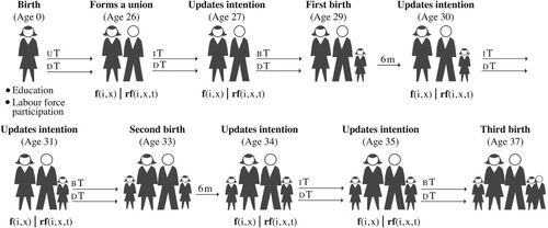
At this point, the model also produces two waiting times: the waiting time until the formation of a union (_UT) and the waiting time until death (_DT). These events compete with each other, meaning that the event with the shortest waiting time is realized. The event that comes first in our example is the formation of a cohabiting union. The age at which this woman forms a union (26) is influenced by the length of time she spends in the educational system, which depends on her educational level.

At union formation, the newly formed couple decide how many children they will try to have; that is, the couple define their desired family size D, which will remain fixed throughout their reproductive trajectory. In defining their desired family size, this couple will take into account existing social norms regarding the ideal number of children, but also whether both members of the couple work outside the home. Note that although only women are simulated, the presence of a working partner is assumed for those that form a union, which implies that after a union is formed, we can think of the couple (instead of the woman) as the ‘agent’ in the model.

Going back to our example, given that our hypothetical woman works, the couple will tend to prefer a family size that is smaller than the existing norm. Although the prevailing ideal at the time (calendar year 1966) is to have three children, they decide to have two.

At union formation, they must decide whether they will try to conceive a child in the next year. The couple in our example decide not to have a child in their first year of cohabitation, which implies that they also try to avoid an unplanned conception.

In our example, they manage to avoid an unplanned pregnancy during their first year of marriage. Now the waiting time until death competes with the waiting time until the moment at which the couple will update their intention and make a new decision _IT, twelve months later. At the end of this twelve-month period, the partners decide to try for a child. When they succeed in conceiving, a waiting time until birth _BT is generated. This results in a first birth when our hypothetical woman is 29 years old. The occurrence of this birth temporarily depresses the intention to have another child.

After the partners return to being exposed to the risk of conception, they decide not to have another child in the first and second years after the first birth. However, in the second year, they fail to prevent an unplanned conception, which results in the woman having a second child when she is 33 years old. When the woman is 37 years old, she has a third child who is unplanned but also unwanted, as the couple have already achieved their desired family size of two children.

Desired family size

As can be appreciated in the example, decisions are an important driver of reproductive outcomes in our model. We distinguish between two types of decisions: how many children to have (long-term preferences) and when to have them (short-term intentions).

In the simulation the desired family size D of woman i is formed immediately after a union is established and is derived from a Gamma distribution (see equation (1)). Gamma provides a good fit to the distribution of family size preferences, which tends to be positively skewed with mode in the range from one to three, depending on the country and time period, and to show a right tail formed by a decreasing number of responses associated with larger family sizes (based on analyses of data from the Integrated Values Surveys; Inglehart et al. 2018).

Based on the assumption that couples in which both partners work will tend to prefer a smaller family, we make the desired family size dependent on the woman’s labour force participation (active/inactive). Our model for D_i also takes into account the fact that individuals live in a society with a given set of norms and that these social norms influence their preferences as much as their individual characteristics do.

In practice, the desired family size D_i of the couple in the model is obtained by rounding to the nearest integer a number drawn from a truncated Gamma distribution with expected value $E_G$ as follows: (1) $\begin{array}{c}{E}_G={\overline{D}}_{t\left[i\right]}\cdot \left(1+{\left(-1\right)}^{w_i}\cdot \left(1-p_{t\left[i\right]}\right)\cdot \delta \right)\end{array}$(1) where t[i] is the time at union formation for woman i, and ${\overline{D}}_{t\left[i\right]}$ is the average desired family size for all women of reproductive age at time t[i], representing the existing social norm regarding the ideal family size at a given time. The amount by which E_G departs from this norm is given by (−1)^w_i· (1 − p_t[i]) · δ, where w_i is a dummy variable indicating the labour force status of woman i (0 = inactive, 1 = active); p_t[i] is the proportion of women in the population who share her labour force participation status, and δ is therefore the maximum proportional departure from the norm. The implication of the (1 − p_t[i]) term is that the larger the fraction of the population that shares her labour force participation status, the closer to the existing social norm the woman will be. For instance, in the extreme case of a homogeneous population of inactive women, the deviation from the norm will be 0 if newly cohabiting woman i is inactive and δ if she is active.

By considering the deviation from existing family size norms, the proposed model represents the evolution of preferences as a path-dependent process, a dependency that results from a feedback loop between the behaviour of previous cohorts, expressed as an aggregate-level societal norm, and the decisions taken at the micro levels by individuals in subsequent cohorts.

Intentions

While the desired family size D_i determines the attempted final parity, we define an intention I_i,t, which plays a role in determining the timing and likelihood of each specific birth. More specifically, the intention I_i,t is the probability that a couple will decide to try to have a child in the next year. The strength of the intention depends on individual, fixed characteristics, but also on the time elapsed since the previous birth ($d_{i,t}$).

For a couple that have achieved their desired family size, I_i,t= 0. Otherwise, their intention is given by: (2) $\begin{array}{c}{I}_{i,t}=\left({\text{β}}_i-{\omega }_i\cdot w_i\right)\left(1-e^{-\lambda \cdot d_{i,t}}\right)\end{array}$(2) where β_i is a baseline that represents the probability of deciding to have a child in a given year for a non-working woman who has not had a child recently and not yet achieved her desired family size.

For working women, the intention also depends on education through ω_i, that we define as: (3) $\begin{array}{c}{\omega }_i={\displaystyle \frac{\eta }{1+\exp \left(\int ϵ\cdot \left(y_i-\tau \right)\right)}}\end{array}$(3) This formulation implies that a penalty on the intention I_i,t exists for women who work ($\eta$), but that this penalty is reduced for those who are more educated. Larger values of τ imply that more years of education $y_i$ are needed to reduce the penalty. A very large value of τ implies that there is no positive effect of education on the intention to have a child.

By allowing education to have a neutral-to-positive effect on the intention to have a child, we account for the mechanisms through which higher educational attainments ease the decision to have a child for a woman who works and has not yet achieved her desired family size. These include the increased ability to outsource childcare, reduce economic uncertainty, negotiate the division of housework, and mobilize personal and familial resources to strike a better balance between work and family.

Finally, the last term in equation (2) models how the intention is affected by d_i,t, the time elapsed since the last birth. In this case, we assume that there is a strong penalty immediately after childbirth that decays over time.

Conception risks

When a couple decide to have a child, their waiting time to conception _CT is determined by their risk of conception. This implies that a couple’s intention is independent from their actual risk, or ability, to conceive. Following earlier models, we represent the risk to conception through the notion of fecundability. In the absence of contraception, fecundability is highest among young couples, and it decreases with age as the frequency of intercourse and biological capacity to conceive decline.

As we model in continuous time, we define fecundability as the instantaneous risk of conception. Specifically, instantaneous fecundability is defined as: (4) $\begin{array}{c}{f}_{i,x}={\displaystyle \frac{\varphi }{1+\exp \left(\kappa \cdot \left(x_i-\gamma \right)\right)}}\end{array}$(4) We fix the value of ϕ, the maximum instantaneous fecundability, at 0.22 per month so as to obtain a 0.93 probability of conceiving within a year ( = 1−e^−12·ϕ). This corresponds to a monthly fecundability of 0.20 ( = 1−e^−ϕ), a value consistent with those reported in the literature for non-contracepting young couples (Bongaarts and Potter 1983; Leridon 2004). Equation (4) specifies that instantaneous fecundability decreases at rate κ as the age x_i of woman i starts to approach age γ. The values for κ and γ are calibrated to fit the pattern of the evolution of fecundability with age proposed by Coale and Trussell (1974) (see Appendix, section A4).

If the partners decide not to have a child in the next twelve months, they will be at risk of an unplanned conception during this period due to ‘residual fecundability’, defined as: (5) $\begin{array}{c}r{f}_{i,x,t}=f_{i,x}\cdot c_{i,t}\cdot a_i\end{array}$(5) where c_i,t ∈ [0, 1] represents the fecundability-reducing effect (effectiveness) of the contraceptive methods available to woman i at time t: c_i,t= 0 means perfect effectiveness, while c_i,t= 1 means complete ineffectiveness. Effectiveness is defined by: (6) $\begin{array}{c}{c}_{i,t}={\displaystyle \frac{{\left(\rho /y_i\right)}^{\alpha }}{1+e^{r\cdot \left(t-\left(\psi -y_i\right)\right)}}+\upsilon }\end{array}$(6) For a given educational attainment level (fixed y_i), the evolution of c_i,t through calendar time is simply a decreasing logistic function with maximum value (ρ/y_i)^α, inflection point ψ − y_i, and steepness r, to which is added a constant υ, the effectiveness of the best contraceptive methods. This definition reflects the notion that although the effectiveness of contraceptive methods improves over time for all women, more educated women adopt efficient contraceptive methods more readily.

Finally, the last term in equation (5), a_i is equal to one if couple i have not yet achieved their desired family size and equal to fixed value a if the couple have already achieved their desired family size. The assumption here is that the partners will intensify their efforts to prevent additional births after they have reached their goal.

If the waiting time until conception (planned or unplanned) _CT is shorter than twelve months, a waiting time until birth _BT is created by adding 270 days of gestation to _CT. Following the birth, there is a period of six months that corresponds to the period of postpartum subfecundity, abstinence, and increased contraceptive use with the aim of avoiding dangerously close births. After this period of time, the couple will go back to being exposed to the risk of a new conception.

If no conception occurs within the next twelve months, our couple will update their intentions again at the end of that period. At that point, the partners will either decide to try to have a child in the next year or they will be subject to the risk of an unplanned birth.

An empirical application

In this section, we test whether the Comfert model can capture fertility change actually observed in the real world.

Input data

Although the structure outlined in the previous section can be adapted to different contexts and time periods, here we focus on post-baby-boom fertility trends in Europe. It is well known that in this region and time period, the Total Fertility Rate (TFR) showed a general pattern of accelerated decline and stabilization, with strong variation between countries in both the timing of each phase and the level of fertility throughout the transition. This transition was driven by the confluence of a myriad of forces, but there are three key processes that stand out from the rest: the diffusion of effective contraceptive methods, the very rapid expansion of higher education, and the large-scale entry of women into the labour market.

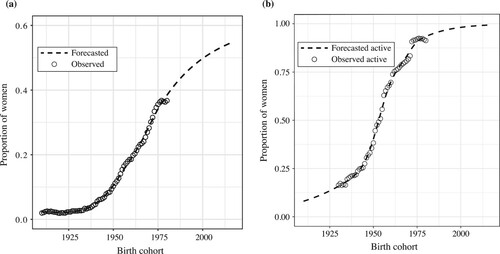
Spain, on which we focus for the empirical application exercise in this section, is a case in point. Figure 3 shows the observed and forecasted proportions of women with tertiary education and proportions of women participating in the labour market (both by birth cohort) computed from census microdata (Minnesota Population Center 2018). The effects of these changes on the transformation of reproductive behaviour cannot be overstated. The virtual disappearance of the breadwinner model is clearly linked to the rapid decline in the desired number of children, and the expansion of education has contributed to the shortening of the period of exposure to the risk of childbearing by significantly postponing the beginning of the family building process.

Figure 3 (a) Tertiary education and (b) labour force participation: Observed and forecasted values for women in Spain, by birth cohort (1910–2017)

Notes: Panel (a) shows the proportion of women with tertiary education by birth cohort. We consider only women aged 30 or older at the time of the census. Panel (b) shows the proportion of economically active (employed + unemployed) women aged 30–55 at the time of the census, by birth cohort. Note that although the univariate distribution is presented here to represent the extent of the changes in the labour force better, we consider the proportions in the labour market by educational attainment when assigning probabilities in the model.

Source: Observed data from four rounds of the Spanish census conducted between 1981 and 2011; forecasted data by authors.

To capture the effects of the expansion of higher education and the transformation of women’s roles, we run our simulation for cohorts born 1910–2017, which allows us to produce period fertility indicators from 1960 to the present. The distance between the simulated and observed indicators is the base of the estimation procedure as explained in the next subsection.

Estimation

As mentioned earlier, the development of likelihood-free estimation methods is one of the main factors behind the growth in the use of computational models in several disciplines. The objective of these methods is to find the combination of parameter values that produces simulated data that most closely resemble the observed data.

The approach we use was proposed by Gutmann and Corander (2016) and uses Bayesian optimization to perform an efficient sequential search of the parameter space. This approach was developed to reduce computation time when, as for our model, simulating model output is time consuming; it does this by focusing on the region of the parameter space where the distance between simulated and observed data tends to be small.

Here we search for the combination of parameter values that reduces the distance between the model output and observed data from Spain. Specifically, let X ⊂ R^q be the parameter space, where q is the number of parameters. At a given combination of parameter values θ ∈ X, we compute Δ_θ the mean squared error (MSE) at this location as a weighted mean of the MSEs for three vectors:

• Age-specific fertility rates (ASFRs) between ages 14 and 50 for the period 1960–2016; available from the Human Fertility Database (2011).

• Average ideal number of children; obtained from Sobotka and Beaujouan (2014).

• Cohort completed fertility by education; obtained from Zeman et al. (2014).

The objective of the estimation procedure is to find the region of the parameter space where the distance Δ_θ is smallest. The basic idea is to proceed sequentially, taking a sample of k locations θ₁, … , θ_k from X and computing Δ_θ1, …  Δ_θk. This evidence is then used to decide where to search next in the parameter space. The distance Δ_θ is then computed on a new set of locations to be explored.

To avoid the need to compute the model at each of these new points, at this stage the model is substituted by an emulator (i.e. a model of the functional relationship between the model parameters and the distance). Specifically, we fit a Gaussian process regression using the R package mlegp (Dancik and Dorman 2008). (For the use of Gaussian process emulators in the context of demographic simulations, see Hilton and Bijak 2017).

The emulator provides predictions of the distance at any combination of parameters, and the decision of where to search next is made using a specific selection criterion or acquisition function. Following Gutmann and Corander (2016) we use a lower confidence bound criterion, which balances exploitation, selecting the locations with best expected values, and exploration, selecting locations where the uncertainty is higher.

The basic operations of the procedure are presented in pseudocode in Box 1.

Box 1 Pseudocode: estimation algorithm

Obtain an initial sample of X of size n₀, θ₁, … , θ_n0

Compute Δ_θ1, … , Δ_θn0

Set n = n₀

While n ≤ N do

Map the relationship θ → Δ_θ with a Gaussian process emulator G(·)

Obtain a new sample of X of size n^∗

Obtain predictions for G(θ_k) k = 1, … , n^∗

Compute acquisition function A(·)

Obtain the new locations to be explored θ_j

Compute Δ_θj

Increment n

end While

Return:

The value of θ that minimizes Δ_θ; or

A fraction p of θ values with lowest Δ_θ

Results

We now test the capacity of our model to fit observed fertility trends in Spain. Table 1 shows the estimated values of the model parameters obtained as described in the previous section, as well as those obtained from different sources (e.g. fecundability parameters).

Table 1 Model parameters and values best fitting data from Spain

Name	Domain	Equation	Description	Value	Source
δ	Desired family size	1	Effect on Di of working	0.64	Estimated
β	Intention	2	Baseline intention	0.8	Fixed
λ	Intention	2	Rate of reduction in penalty after pregnancy	2.5e−8 s^−^1	Fixed
η	Intention	3	Penalty on intention of working	0.58	Estimated
τ	Intention	3	Years of education after which η is reduced	21.3 yr	Estimated
ϵ	Intention	3	Speed at which η is reduced	0.53 yr^−^1	Fixed
ϕ	Fecundability	4	Maximum fecundability	0.22 mo^−^1	Fixed
γ	Fecundability	4	Inflection point of decline (age)	38.5 yr	Fixed
κ	Fecundability	4	Speed of decline with age	0.6 yr^−^1	Fixed
a	Contraception	5	Additional effect due to achieved Di	0.07	Fixed
ρ	Contraception	6	Minimum effect on conception risk	0.03	Estimated
υ	Contraception	6	Maximum effect on conception risk	0.55	Estimated
ψ	Contraception	6	Inflection year in the diffusion process	1977	Estimated
r	Contraception	6	Speed of the diffusion	0.21 yr^−^1	Estimated
α	Contraception	6	Differential access/use by education	0.20	Estimated
ξ	Age at union formation	7	Time to union after schooling	7.03 yr	Estimated

Notes: The baseline intention β was set a value lower than one to consider other effects not explicitly modelled that might impose a penalty on the intention. ‘yr⁻¹’ refers to per year, ‘mo⁻¹’ refers to per month, and ‘s⁻¹’ refers to per second.

Source: Estimates for γ and κ were derived from the scheduled developed by Coale and Trussell (1974) as explained in the Appendix. Estimates for the rest of the fixed parameters were obtained by calibration.

The results presented in Figure 4 are obtained by running the model using the input data and the combination of parameter values in Table 1. The model outputs simulated reproductive trajectories at the individual level, from which it is possible to compute the evolution of any fertility indicator of interest.

Figure 4 Simulated and observed key fertility indicators for women in Spain (a) Total fertility; (b) Cohort completed fertility; (c) Mean age at birth

Note: We present the results of ten simulations with the same combination of parameter values (small dots) and their mean (large, light grey dots).

Source: Observed data from the Human Fertility Database; simulated data by authors.

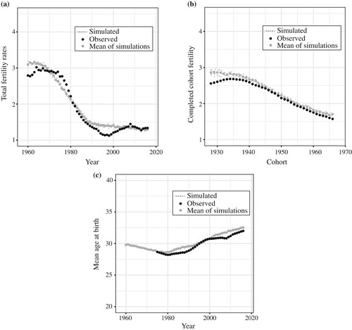
The simulated TFR (Figure 4(a)) closely follows the decline observed since the mid-1970s and the subsequent stabilization from the mid-1990s onward. In its current form, the model does a better job in reproducing variation in the timing of fertility associated with cohort processes (Figure 4(b)) than it does in capturing period effects, that is, shorter-term influences associated with, for example, the economic cycle or migration flows (Figure 4(a)). This likely explains the discrepancies between the predicted and the observed TFR. Indeed, the periods with larger discrepancies coincide with periods characterized by marked timing changes. This pattern can also be seen in Figure 4(c), which depicts the observed and simulated mean ages at birth.

In most cases, these changes are associated with: (1) exceptional situations in the labour market, including the recuperation of employment rates from the mid-1990s until the Great Recession of 2008; and (2) the influence of migration flows, which contributed to a slowdown in the pace of postponement, as we describe in more detail shortly.

The information provided by the model can be obtained at any level of disaggregation. Figure 5 presents the same information contained in the three indicators shown in Figure 4, but this time in the form of ASFRs. Over time, the simulated ASFRs move downward and shift to the right following the observed rates, which indicates the decline and postponement of fertility. In the model, the reduction in ASFRs results from the combination of declines in desired family size and in proportions of unplanned births. By contrast, the shift to later ages is produced not only by the lengthening of the period spent in education (which, in turn, leads to later ages at union formation), but by the increasing ability to space births as a consequence of improved control over the reproductive process.

Figure 5 Simulated and observed ASFRs for women in Spain, selected years (a) 1960; (b) 1980; (c) 2000; (d) 2016

Note: We present the results of ten simulations with the same combination of parameter values (small dots) and their mean (large, light grey dots).

Source: As for Figure 4.

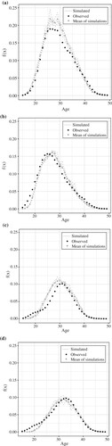
The predictions from the model start to diverge from the observations around 2000, when an early bulge in the schedule becomes visible (Figure 5(c)). This mildly bimodal pattern has been observed in other European countries as well and appears to have been driven by immigration flows (Burkimsher 2017). As the model assumes a closed population, these changes in the fertility schedule associated with the incorporation of women with an earlier fertility pattern into the population cannot be captured.

Towards a unified programme

In 1974, the Mindel C. Sheps Award was set up to recognize contributions in mathematical demography and demographic methods. In the following 15 years, most award recipients were recognized for their work on the analysis of fertility and reproduction dynamics. Many had indeed been instrumental in the development of the early models of the reproductive process. By contrast, the vast majority of award recipients after 1990 made their most significant contributions on other topics. During the initial years, fertility researchers had of course continued to improve the understanding of fertility dynamics, but mostly through solid descriptive analysis and statistical modelling of microdata; the approach promoted by Mindel Sheps seems to have migrated to different areas of demographic research, despite its considerable merits.

In the present paper, we outlined the history of this change in the zeitgeist of fertility research, describing how after a few decades of active development, the tradition of family building models gradually disappeared. We highlighted several external factors that led to this shift, such as the increased availability of individual-level data and the use of standard statistical models. But we also noted that at least equally important were the analytical limitations of the models themselves, which never attempted to transcend the study of physiological factors and systematically incorporate the largest source of variation in a regulated fertility context, namely preferences and intentions.

One of our main objectives was to describe how the convergence of various trends and ideas has created the conditions for a fruitful return to mechanistic modelling in fertility research. These trends include a wider use of more flexible simulation approaches that are better suited to model decisions and intentions; the development of statistical frameworks that allow for inference and uncertainty estimation in complex computational models; and the rapid technological progress in both computing power and programming tools that has made it relatively simple to implement and compute large simulation models.

These ideas have already been explored by a small community of researchers in recent years, in the context of different demographic problems. Although a few computational models that seek to explain fertility dynamics have also been developed as part of this process, no attempt has so far been made to represent the entire sequence of events and decisions involved in the reproductive process. Moreover, these endeavours have remained disconnected from the existing modelling tradition in fertility research, paying limited attention to important concepts such as the notion of fecundability, central in earlier models of the reproductive process and still useful nowadays.

Further, after tracing back the history of family building models, and identifying the reasons for their disappearance and opportunities for their re-emergence, we introduced an example of what a new generation of family building models could look like and tested its ability to describe observed macro-level fertility patterns. The algorithm we presented here takes the distributions of educational attainment and labour force participation as inputs, and it outputs a set of simulated maternity histories. The model offers a representation of the main mechanisms that shape the reproductive process in contemporary developed societies with regulated fertility regimes. This can be thought of as a data-generating process, from which information can be simulated on the number of children desired, the number of children born, the maternal age at each birth, and whether each of these births was planned, mistimed, or unwanted. After these maternity histories have been collected (simulated), any standard fertility index (e.g. TFR, cohort fertility indicators, or parity progression ratios) can be computed and compared with the observed values.

By focusing on the determinants of events and decisions in the reproductive process, we can go beyond the description of trends and provide an explanation of how a given set of micro-level mechanisms can produce the observed trends at the aggregate level, while considering both the intended and unintended processes that make up fertility outcomes. Our model generates the decline and postponement of fertility in post-baby-boom Europe from a combination of three key drivers: (1) the decline in desired family size, as the proportion of couples in which one of the partners is exclusively devoted to housework continues to shrink; (2) the shortening of the reproductive lifespan, as individuals spend a larger fraction of their lives in the education system; and (3) the reduction in unplanned births, as information on effective contraceptive methods spreads through the population.

However, the production of qualitative insights should not be the exclusive goal of this new generation of family building models. The combination of data-driven approaches with solid statistical frameworks for parameter estimation and model evaluation should give rise to computational models of demographic dynamics that are as able to explain the past as they are to predict the future. While forecasting using a micro-level mechanistic model involves a substantially higher level of complexity than extrapolating from a macro-level statistical model, it also incorporates significantly more information and can thus yield a substantially improved understanding of future trends.

In conclusion, we believe that the recovery and further development of the individual-level modelling tradition in fertility research can bring about a more integrated, coherent division of labour in which: (1) theory is more rigorously postulated in the form of precisely defined models; (2) the development of these domain-specific models relies on the information generated by empirical and descriptive research; and (3) these larger computational models can themselves be estimated, thereby uncovering a number of mechanisms and quantities that have remained out of reach until now.

Notes

1 Please direct all correspondence to Daniel Ciganda, Max Planck Institute for Demographic Research, Konrad Zuse Str. 1, Rostock 18057, Germany; or by Email: [email protected].

2 We would like to thank Thomas Burch for his insightful comments on an earlier version of this article.

Appendix. Additional model description

A1. Age at union formation

To keep things simple, the preferences, intentions, and risks that control the reproductive process are assumed to operate only after the formation of a cohabiting union. The age at which this event occurs is therefore of great importance. We follow previous studies that have successfully approached the empirical distribution in age at marriage using the log-normal distribution (Mode 1985), where: (7) $\begin{array}{c}\ln \left(M_i\right)\sim N\left({\mu }_i,{\sigma }^2\right)\end{array}$(7) with µ_i= y_i + ξ, where y_i is the number of years of education of woman i, and parameter ξ is the average waiting time (in years) to the formation of a cohabiting union after the end of the schooling period.

A2. Death

The waiting time until death is sampled using the inverse distribution function method (for a description of the method, see Willekens 2009), where the distribution of waiting times until death is reconstructed using age-specific cohort mortality rates.

A3. Pseudocode

Most earlier computational models were built on a discrete-time framework in which time advances in arbitrary and equally spaced time units, and the state of the system is updated at each of these iterations. We use a discrete-event framework (Zeigler et al. 2000) in which time advances with the realization of events. At each iteration, the algorithm finds the event with the shortest waiting time from a list of all possible events for the entire population of simulated individuals. After the realization of the next event, the state of the system and the clock are updated and the simulation can continue to the next run. In demography this approach is known as microsimulation in continuous time (see Willekens 2009).

The pseudocode in Box A1 describes the basic operation of the Comfert algorithm. The entire process is described by four events: start of a cohabiting union, evaluation of whether or not to have a child, childbearing, and death.

Box A1 The Comfert algorithm (pseudocode)

read input data educational attainment (cohort) labour force participation by education (cohort) initialization generate wts to birth in the first year While time < end time do choose next event → n_event update clock update ages & waiting times if n_event = birth then   if girl then    add to population    assign:    educational attainment    years in education    labour force participation    wt to union    wt to death    wt to evaluate == Inf   end   update indicators of mother:   age at birth   no. children   no. children left   wt to evaluate end if n_event = death then  remove from the population end (continues at top of right-hand column)

if n_event = union formation then   assign desired family size Di   compute intention Ii,t   if Ii,t > x ∼ U(0, 1) then     wt conception → fi,x   else     wt conception → rfi,x,t   end   if wt conception > 1 year then    wt evaluate = = 1 year   end end if n­_event = evaluate then   update intention Ii,t   if Ii,t > x ∼ U(0, 1) then     wt conception → fi,x   else     wt conception → rfi,x,t   end   if wt conception > 1 year then     wt evaluate == 1 year   end end if year change then   remove those with age > max_age   compute indicators. end end While save output asfrs; unplanned births; desired family size. end

wt = Waiting time; n_event = Next event; max_age = Age at end of reproductive period (50); asfrs = Age-specific fertility rates; end time = Last year for which model is run; f = Fecundability; rf = Residual fecundability.

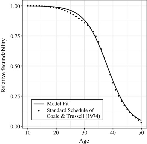
A4. Decline in fecundability with age

In one of the early attempts to understand the decline in fecundability with age, Coale and Trussell (1974) derived a standard schedule of marital fertility through the study of ASFRs in a group of populations with a natural fertility regime. They noted that although the fertility levels in these populations were different, a clear pattern of decline could be identified, which they summarized in the schedule depicted by the points in Figure A1. The solid line corresponds to the fit of our model (see equation (4)).

Figure A1 Relative decline in fecundability with age

Source: Coale and Trussell (1974). Model fit by authors.

A5. Additional measures of model fit

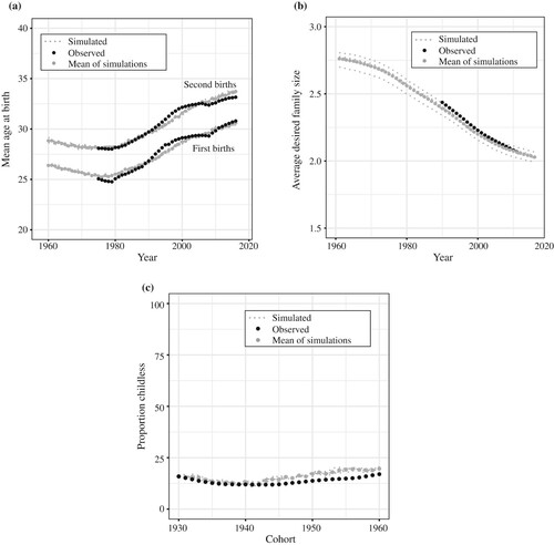
Figure A2 shows three additional fertility indicators to illustrate model fit, supplementing those shown in Figures 4 and 5.

Figure A2 Simulated and observed selected fertility indicators for women in Spain. (a) Mean age at first and second birth; (b) Mean desired family size; (c) Proportion childless

Notes: Panel (a) shows period mean ages at birth for parities one and two since 1960. Panel (b) shows the fit to the average desired family size, also from 1960. Panel (c) shows the proportion of women that remained childless at the end of their reproductive life from the cohort of women born in 1930 until the last cohort observed.

Source: Simulated data by authors; observed data from: (a) Human Fertility Database; (b) Sobotka and Beaujouan (2014); (c) Esteve et al. (2016).

References

- Aparicio Diaz, B., T. Fent, A. Prskawetz, and L. Bernardi. 2011. Transition to parenthood: The role of social interaction and endogenous networks, Demography 48(2): 559–579. doi:10.1007/s13524-011-0023-6
- Barrett, J. C. 1969. A Monte Carlo simulation of human reproduction, Genus 25(1/4): 1–22. https://www.jstor.org/stable/29787859
- Barrett, J. C. 1971. Use of a fertility simulation model to refine measurement techniques, Demography 8(4): 481–490. doi:10.2307/2060684
- Beaumont, M. A. 2010. Approximate Bayesian computation in evolution and ecology, Annual Review of Ecology, Evolution, and Systematics 41: 379–406. doi:10.1146/annurev-ecolsys-102209-144621
- Beaumont, M. A. 2019. Approximate Bayesian computation, Annual Review of Statistics and its Application 6: 379–403. doi:10.1146/annurev-statistics-030718-105212
- Billari, F. C., T. Fent, A. Prskawetz, and J. Scheffran. 2006. Agent-based Computational Modelling: Applications in Demography, Social, Economic and Environmental Sciences. Heidelberg: Physica-Verlag Heidelberg.
- Billari, F. C., F. Ongaro, and A. Prskawetz. 2003. Introduction: Agent-based computational demography, in Agent-based Computational Demography. Dordrecht: Springer, pp. 1–17.
- Bongaarts, J. 1977. A dynamic model of the reproductive process, Population Studies 31(1): 59–73. doi:10.1080/00324728.1977.10412747
- Bongaarts, J., and R. E. Potter. 1983. Fertility, Biology, and Behavior: An Analysis of the Proximate Determinants. Amsterdam: Academic Press.
- Brass, W. 1958. The distribution of births in human populations in rural Taiwan, Population Studies 12(1): 51–72. doi:10.1080/00324728.1958.10404370
- Burch, T. K. 2018. Does demography need differential equations?, Model-Based Demography. Dordrecht: Springer, pp. 79–94. https://link.springer.com/chapter/10.1007/978-3-319-65433-1_5
- Burkimsher, M. 2017. Evolution of the shape of the fertility curve: Why might some countries develop a bimodal curve?, Demographic Research 37: 295–324. doi:10.4054/DemRes.2017.37.11
- Ciganda, D. and F. Villavicencio. 2016. Feedback mechanisms in the postponement of fertility in Spain, in André Grow and Jan Van Bavel (eds), Agent-Based Modelling in Population Studies. Dordrecht: Springer, pp. 405–435
- Coale, A. J., and T. J. Trussell. 1974. Model fertility schedules: Variations in the age structure of childbearing in human populations, Population Index 40: 185–258. doi:10.2307/2733910
- Coale, A., and J. Trussell. 1996. The development and use of demographic models, Population Studies 50(3): 469–484. doi:10.1080/0032472031000149576
- Colombo, B., and G. Masarotto. 2000. Daily fecundability: First results from a new data base, Demographic Research 3. doi:10.4054/DemRes.2000.3.5
- Connolly, S. R., S. A. Keith, R. K. Colwell, and C. Rahbek. 2017. Process, mechanism, and modeling in macroecology, Trends in Ecology & Evolution 32(11): 835–844. doi:10.1016/j.tree.2017.08.011
- Cox, D. R. 1972. Regression models and life-tables, Journal of the Royal Statistical Society: Series B (Methodological) 34(2): 187–202. doi:10.1111/j.2517-6161.1972.tb00899.x
- Dancik, G. M., and K. S. Dorman. 2008. Mlegp: Statistical analysis for computer models of biological systems using R, Bioinformatics 24(17): 1966–1967. doi:10.1093/bioinformatics/btn329
- Dandekar, V. 1955. Certain modified forms of binomial and Poisson distributions, Sankhyā: The Indian Journal of Statistics (1933-1960) 15(3): 237–250. https://www.jstor.org/stable/i25048241
- Dunson, D. B., B. Colombo, and D. D. Baird. 2002. Changes with age in the level and duration of fertility in the menstrual cycle, Human Reproduction 17(5): 1399–1403. doi:10.1093/humrep/17.5.1399
- Ecochard, R. 2006. Heterogeneity in fecundability studies: Issues and modelling, Statistical Methods in Medical Research 15(2): 141–160. doi:10.1191/0962280206sm436oa
- Esteve, A., D. Devolder, and A. Domingo. 2016. Childlessness in Spain: Tick Tock, Tick Tock, Tick Tock!, Perspectives Demogràfiques 1: 1–4.
- Fent, T., B. A. Diaz, and A. Prskawetz. 2013. Family policies in the context of low fertility and social structure, Demographic Research 29: 963–998. doi:10.4054/DemRes.2013.29.37
- Finkel, A. 2019. To move research from quantity to quality, go beyond good intentions, Nature 566(7744): 297. doi:10.1038/d41586-019-00613-z
- Gardner, M. 1970. Mathematical games, Scientific American 222(6): 132–136. doi:10.1038/scientificamerican0670-132
- Gini, C. 1924. Premières recherches sur la fécondabilité de la femme [Initial Research on the Fecundability of Women], in North-Holland: (ed), Proceedings of the International Mathematical Congress. (Vol. 2.). Toronto.
- Grow, A. and J. Van Bavel (eds). 2016. Agent-Based Modelling in Population Studies: Concepts, Methods, and Applications (Vol. 41). Dordrecht: Springer.
- Gutmann, M. U. and J. Corander. 2016. Bayesian optimization for likelihood-free inference of simulator-based statistical models, The Journal of Machine Learning Research 17(1): 4256–4302.
- Hartig, F., J. M. Calabrese, B. Reineking, T. Wiegand, and A. Huth. 2011. Statistical inference for stochastic simulation models - Theory and application, Ecology Letters 14(8): 816–827. doi:10.1111/j.1461-0248.2011.01640.x
- Hegselmann, R., Thomas C. Schelling, and James M. Sakoda. 2017. The intellectual, technical, and social history of a model, Journal of Artificial Societies and Social Simulation 20: 3. doi:10.18564/jasss.3511
- Henry, L. 1953. Fondements théoriques des mesures de la fécondité naturelle [Theoretical basis of measures of natural fertility], Revue de l’Institut International de Statistique / Review of the International Statistical Institute 21(3): 135–151. doi:10.2307/1401425
- Henry, L. 1972. On the Measurement of Human Fertility: Selected Writings of Louis Henry. Amsterdam: Elsevier Publishing Company.
- Hilton, J. and J. Bijak. 2017. Design and analysis of demographic simulations, in André Grow and Jan Van Bavel (eds) Agent-based Modelling in Population Studies. Dordrecht: Springer, pp. 211–235.
- Human Fertility Database. 2011. Human Fertility Database.
- Inglehart, R., C. Haerpfer, A. Moreno, C. Welzel, K. Kizilova, J. Diez-Medrano, M. Lagos, P. Norris, E. Ponarin, and B. Puranen et al. (eds). 2018. World Values Survey: All Rounds - Country-Pooled Datafile. Madrid: JD Systems Institute. Available: https://www.worldvaluessurvey.org/WVSDocumentationWVL.jsp
- Klabunde, A., S. Zinn, F. Willekens, and M. Leuchter. 2017. Multistate modelling extended by behavioural rules: An application to migration, Population Studies 71(sup1): 51–67. doi:10.1080/00324728.2017.1350281
- Le Bras, H. 1993. Simulation of change to validate demographic analysis, in David Sven, Reher and Roger S. Schofield (eds) Old and New Methods in Historical Demography. Oxford, England: Clarendon Press, pp. 259–280.
- Leridon, H. 2004. Can assisted reproduction technology compensate for the natural decline in fertility with age? A model assessment, Human Reproduction 19(7): 1548–1553. doi:10.1093/humrep/deh304
- Minnesota Population Center. 2018. Integrated public use microdata series, International: Version 7.0.
- Mode, C. J. 1985. Stochastic Processes in Demography and Their Computer Implementation (Vol. 14). Dordrecht: Springer Science & Business Media.
- Orcutt, G. H. 1957. A new type of socio-economic system, The Review of Economics and Statistics 39: 116–123. doi:10.2307/1928528
- Perrin, E. B. and M. C. Sheps. 1964. Human reproduction: A stochastic process, Biometrics: 28–45. doi:10.2307/2527616
- Potter, R. G. 1972. Additional births averted when abortion is added to contraception, Studies in Family Planning 3(4): 53–59. doi:10.2307/1965360
- Potter, R. G. and J. M. Sakoda. 1966. A computer model of family building based on expected values, Demography 3(2): 450–461. doi:10.2307/2060170
- Ridley, J. C. and M. C. Sheps. 1966. An analytic simulation model of human reproduction with demographic and biological components, Population Studies 19(3): 297–310. doi:10.1080/00324728.1966.10406018
- Sakoda, J. M. 1971. The checkerboard model of social interaction, The Journal of Mathematical Sociology 1(1): 119–132. doi:10.1080/0022250X.1971.9989791
- Schelling, T. C. 1971. Dynamic models of segregation, The Journal of Mathematical Sociology 1(2): 143–186. doi:10.1080/0022250X.1971.9989794
- Sheps, M. C., J. A. Menken, and A. P. Radick. 1973. Mathematical Models of Conception and Birth. Chicago: University of Chicago Press.
- Singh, S. 1963. Probability models for the variation in the number of births per couple, Journal of the American Statistical Association 58(303): 721–727. doi:10.1080/01621459.1963.10500882
- Singh, S., B. Bhattacharya, and R. Yadava. 1974. A parity dependent model for number of births and its applications, Sankhyā: The Indian Journal of Statistics, Series B 36(1): 93–102. https://www.jstor.org/stable/25051886
- Sobotka, T. and E. Beaujouan. 2014. Two is best? The persistence of a two-child family ideal in Europe, Population and Development Review 40(3): 391–419. doi:10.1111/j.1728-4457.2014.00691.x
- Van de Kaa, D. J. 1987. Europe’s second demographic transition, Population Bulletin 42(1): 1–59.
- Venkatacharya, K. 1971. A Monte Carlo model for the study of human fertility under varying fecundability, Social Biology 18(4): 406–415. doi:10.1080/19485565.1971.9987949
- Willekens, F. 2009. Continuous-time microsimulation in longitudinal analysis, in Asghar Zaidi, Ann Harding, and Paul Williamson (eds), New Frontiers in Microsimulation Modelling. London: Routledge, pp. 353–376.
- Willekens, F. 2014. Multistate Analysis of Life Histories with R. Dordrecht: Springer.
- Xie, Y. 2000. Demography: Past, present, and future, Journal of the American Statistical Association 95(450): 670–673. doi:10.1080/01621459.2000.10474248
- Zeigler, B. P., T. G. Kim, and H. Praehofer. 2000. Theory of Modeling and Simulation. Amsterdam: Academic Press.
- Zeman, K., Z. Brzozowska, T. Sobotka, E. Beaujouan, and A. Matysiak. 2014. Cohort Fertility and Education database. Methods protocol. Available at www.cfedatabase.org (last accessed on 10.4. 2017). Technical report, Vienna Institute of Demography.