Population decline and changes in food store access

ABSTRACT

I examine how neighbourhood-level food store access, proxied by distance to the nearest food store, changed in Sweden between 2000 and 2013, and how this change is correlated with changes in potential market size, proxied by population density. I find that distance has increased in rural and more affluent neighbourhoods. Furthermore, an increase in distance is negatively correlated with an increase in population density and is most pronounced in rural areas. The results are driven by the growing, rather than the declining, regions. Since the latter have often been a target for subsidies over the years, this could suggest that the aid may have had an impact.

KEYWORDS:

• retail
• food stores
• panel data
• access
• Sweden
• spatial analysis

JEL:

• C23
• D22
• L81
• R11

1. INTRODUCTION

In many developed economies, the spatial concentration of both retail (Dawson, 2006) and population (Turok & Mykhnenko, 2007) has increased over time. In parallel, many regions have experienced a population decline. When the market size drops too low, commercial services such as food stores are forced to close or relocate. Residents who remain must now travel a greater distance to obtain the same services, which incurs costs in terms of time and transportation (Hodge et al., 2000), and decreases the attractiveness of the area for future inhabitants. Thus, population decline puts a strain on service delivery, a trend that has been viewed with growing concern in many countries (Grediaga & Freshwater, 2010). The process of a dispersed spatial configuration of people is also a problem in the urban environment because it increases the costs of service provision (Varela-Candamio et al., 2019) and thus decreases the density and availability of grocery stores (Hamidi, 2020).

Low food access can be considered a problem from a variety of perspectives. For instance, an area where there are few or no food stores is hypothesized to be a contributor to lower health because it reduces the consumption of healthy foods. However, this hypothesis has received mixed support (e.g., Allcott et al., 2019; Larson et al., 2009).

In addition to its direct function as a provider of groceries, food stores – particularly in rural areas – are argued to play important roles as local hubs (Clarke & Banga, 2010) and as providers of additional services and goods such as postal services and drugstore products (SOU, 2015). Additionally, they may stimulate business connections by creating demand and growing local suppliers (Ilbery & Maye, 2006). In remotely located settlements, where there are few alternative providers, the local food store is therefore often seen as an integral part of the community (Marshall et al., 2018). The food environment has recently received renewed interest in the context of food security in the COVID-19 pandemic. As the mobility of consumers has been severely restricted in many countries, the necessity of an adequate local food environment has become glaringly apparent. Against this backdrop, the presence of a food store is arguably of direct and indirect value.

Ensuring access to grocery stores and similar services has been one of the target areas of European Union (EU) policy since 2007, and in Sweden subsidies have been in place since 1994 (Swedish Parliament, 2000). Together with other commercial services (e.g., gas stations and postal service points), food stores in areas with declining populations received up to a total of US$51 million between 2002 and 2013 (The Swedish Agency for Economic and Regional Growth, 2015; The Swedish Consumer Agency, 2008).

Research shows that access to food stores varies considerably with socio-economic, locational and demographic factors (e.g., Gordon et al., 2011; Larson et al., 2009; Powell et al., 2007). While the literature on inequalities in food access is large, few studies examine its determinants, and the studies that do (e.g., Hamidi, 2020) use cross-sectional data. Thereby, it is not known how changes in food access are correlated with changes in local conditions, which is necessary to understand so as to address these inequalities.

In this paper I focus on food access by proximity; thus, ‘food access’ in this study refers to the geographical proximity to food stores. I analyse the development in neighbourhood-level food store access as a function of the size of nearby demand while accommodating time-invariant heterogeneity. Thus, I focus on examining changes in food access and the relationship with changes in market size. As such, this study contributes to the literature on understanding how inequalities in food access by proximity emerge. Furthermore, I assess it for regions of different degrees of centrality. It thereby informs policymakers on how food store access has developed in recent times, in what type of regions the change has been most pronounced and hence where there is an enhanced need for interventions.

The dynamics of the Swedish retail market are of particular interest to study because during the period of study of this paper, 2000–13, Sweden was one of the Organisation for Economic Co-operation and Development (OECD) countries with the lowest degree of regulation of retail trade (OECD, 2020). Thus, the location decisions of the food stores in this study may be argued to be influenced by market factors to a relatively high extent. Furthermore, while the rise of online retail may have reduced the relevance of local demand, the size of online grocery retail was at a very modest level in this period, and in 2014 it constituted a mere 1% of total grocery retail sales (The Swedish Trade Federation, 2020). Thereby, one may further assume that in this period the local demand remained of importance for food store location.

This study consists of two parts. In the first part I assess how neighbourhood-level food access – defined as neighbourhood inhabitants’ average distance to the nearest food store – has changed between two points in time, 2000 and 2013, and how it has changed for different socio-economic groups. Thereby I build on Amcoff (2017), where food store access for various socio-economic groups in Sweden is analysed at two points in time, 1998 and 2008. Thus, the first part of the present study merely complements that of Amcoff (2017) by examining a somewhat later period, and by focusing on the neighbourhood level.

In the second part of the analysis, which constitutes the main contribution of this paper, I use a panel dataset covering all Swedish neighbourhoods over a 14-year period to assess the relation between food store access and potential local market size, proxied by population density. Access to food stores is now proxied using the distance from the centroid of a neighbourhood to the nearest food store. The mechanisms at work can be illustrated as follows: when the population density of a neighbourhood increases, the potential local market size increases, which may attract food stores to locate in the area. This results in an increase in the number of food stores within the area, which in turn improves food store access by way of proximity for the inhabitants in the neighbourhood. The resulting model is estimated using a fixed effects spatial econometric framework that accommodates both time-invariant heterogeneity and spatial dependence between neighbourhoods.

However, retail is a recognized amenity in the literature (e.g., Öner, 2017), and since amenities have been shown to influence individuals’ choice of residence (Biagi et al., 2011), the relationship between food retail and population density may be endogenous. Nevertheless, the design of this study builds on the assumption that the direction of the relationship is one where population density affects the location of food stores, although it cannot be proved in the current analysis.

The first part of the analysis reveals that the average neighbourhood-level distance of the residents to the nearest food store has increased by approximately 400 m. The areas in which distance to food stores has increased are primarily socio-economically affluent. Amcoff (2017) found that the socio-economically well-off groups in general had a longer distance to the nearest food store and that the same groups had also experienced an increase in distance during the period; thus, the first part of the present study supports the findings of Amcoff.

The findings from the second part of the analysis indicate that population density is significantly negatively correlated with the distance from the neighbourhood centroid to the nearest food store, with an elasticity of 0.18. Thus, a doubling in population density is correlated with a decrease of 18% in the distance to the nearest food store. Moreover, the correlation is stronger in neighbourhoods located in rural regions than in neighbourhoods located in urban and metropolitan areas. Furthermore, the results appear to be driven by the growing, rather than the declining, regions, as the relationship between density and access is not statistically significant for the latter. Since declining regions have been recipients of subsidies for years, this result could imply that the financial support may have had an impact.

How well do these results translate in an international context? As previously noted, the Swedish retail sector is relatively unregulated compared with other OECD countries; thus, the effects documented in this study may be seen as an upper bound relative to more regulated retail markets, such as the Netherlands and the UK, and a lower bound to, for instance, Latvia (OECD, 2020).

The remainder of the paper is structured as follows. The next section presents the previous literature, followed by the theoretical framework. Sections 4 and 5 present the data and empirical methods, respectively. Section 6 discusses the results, and section 7 concludes the paper.

2. PREVIOUS STUDIES

Disparities in food store access gained attention with the coinage of the term ‘food desert’ in a 1998 report on rising inequalities in the level of health in Britain. The study, conducted by the Social Exclusion Unit (1998), described a pattern of withdrawal of these services in areas where the residents were of poor health and low income (Wrigley, 2002). After the publication of this report, several studies on the topic followed. These involved mapping the extent of inadequate food access and intervention studies where the effects of increased physical access to food retail on health outcomes were examined (e.g., Cummins et al., 2008; Cummins & Macintyre, 2002). The issue also received attention in the United States and gave rise to a large body of literature in a range of research fields, and in the United States government actions were also taken to improve food store availability (Donald, 2013).

In the food desert literature, the focus has been to examine the extent of systematic socio-economic inequalities in food store access, and relatively few inferential studies have examined what may explain the spatial variation in food store location. In the few studies that exist, the definition of spatial access varies. It is common to use a prespecified definition of low food access and model the probability of an area sorting into this category as a function of different market variables. For instance, Dutko et al. (2012) define low food access as an area where at least 500 people and/or 33% of inhabitants reside beyond 1 mile (for urban areas) or 10 miles (for rural areas) from a food store. A similar definition was used by Hamidi (2020). In studies of threshold demand analysis – those that estimate the minimum size of demand needed to maintain a facility – store density is often used (e.g., Chakraborty, 2012; Mulligan et al., 1985).

A variety of variables are often used to model the distribution of food stores, and size of demand, typically proxied by population size or density – is an integral determinant of retail location. In one of the earlier studies, Mulligan et al. (1985) examined the number of food stores in 20 Arizona communities in 1981 and found that population size was positively correlated with the number of stores in a community. More recently, Amin et al. (2020) studied access to healthful (stores that offer a broad variety of healthy foods) food stores in the United States using 2010 census data. They found that areas with lower population densities also tended to have very few to no food stores. Similar findings have been documented by Chakraborty (2012), Dutko et al. (2012) and Hamidi, (2020).

Indications of agglomeration effects of demand, in that size of demand is positively correlated with retail presence but at a decreasing rate, are also documented, for instance, by Parr and Denike (1970) as well as more recently Chakraborty (2012). In the latter, threshold demands, proxied by population, for a variety of retail categories are estimated in 2201 US counties in 2000. In this study, population was found to have a positive but decreasing correlation with the number of food stores.

Not only the local size of demand matters. Places with a high market potential also tend to have a larger stock of retail, thus the size of the demand in neighbouring regions may also influence the presence of food stores. This has been found in several studies. For instance, in Harris et al.’s (1996) study of retail firms in 2126 US communities in 1986, it was shown that the population size of a community had a positive association with the number of grocery retailers, while proximity to metropolitan areas had a negative effect. Similar findings were reported in the Canadian study by Wensley and Stabler (1998), as well as by Chakraborty (2012). However, some studies find no indications of spatial dependencies. Using census data in 1992, Mushinski and Weiler (2002) studied a variety of retail stores in non-metropolitan places in eight US states. Population size had a significant correlation with the number of grocery stores, while proximity to metropolitan areas had no influence. Similar results were found by Thilmany et al. (2005).

The demographic and socio-economic composition of the demand may matter as well. For instance, in Mulligan et al. (1985), the share of the population under age 16 and the share of the population above age 65 were found to be positively correlated with the number of food stores. Harris et al.’s (1996) results showed that income per capita of a community had a positive association with the number of grocery retailers. This was also found by Hamidi (2020), while Mulligan et al. (1985) and Chakraborty (2012) found that income was negatively correlated with the number of food stores, and Mushinski and Weiler (2002) and Thilmany et al. (2005) found no effects of income at all. Other socio-economic factors that have been found to be correlated with store presence are level of education, unemployment, poverty (e.g., Hamidi, 2020) and ethnic composition (e.g., Amin et al., 2020).

Previous studies offer several valuable insights into the patterns of food store location. However, the data that are used only allows for cross-sectional analyses, thus no conclusions can be made regarding how food access changes over time and how these changes correlate with changes in market conditions. The present study contributes with knowledge on this matter, and this knowledge may not be sufficient, but it is necessary in order to address inequalities in food access.

3. THEORY

Using central place theory (CPT), Christaller (1966) and Losch (1964) modelled the uneven pattern of economic activities in space as a function of the consumer’s transport costs and the minimum size of demand required to support an economic function. The theory is based on the notion that places where market agents interact – central places – are allocated in space in a regular pattern.

The distance between central places is determined by the demand and production functions of the consumers and producers. Next to the firm, the consumer’s demand for a good decreases with price. As the distance to the firm grows, the consumer’s demand decreases, and at one point in space, the distance to which is termed the range, it drops to zero and the consumer is supplied by a competitor. Given a uniformly distributed population, the size of the demand that the firm must capture to break even, the threshold demand, is proportional to the radius of the geographical market size, which is termed the threshold distance. If the range is larger than the threshold distance, the firm makes a profit, and more firms will enter the market. If the opposite holds, the firm loses money and consequently leaves the market.

Due to variations in production costs and demand structures, the range and threshold will differ between different types of goods. Frequently bought goods, with a low cost of production – lower order goods – have a shorter range and threshold distance compared with infrequently purchased goods – higher order goods. The result of this relationship is that a regular but sparse pattern of higher order goods firms is layered over a more narrowly spaced pattern of lower order goods firms. Consequently, places with higher order goods firms – higher order places – also house lower order goods firms.

Later contributions (e.g., Isard, 1956) showed that the number of firms in a given area would increase when the density of demand increases. This increase was shown to occur at a decreasing rate (Berry & Garrison, 1958; Parr & Denike, 1970).

Against this backdrop, it is possible to derive a theoretical model that describes the relationship between consumer density and market size. I use the circular market model of Salop (1979) as a point of departure to express the relationship between consumer density $\left(\rho \right)$ and threshold distance $\left(D\right)$. The steps taken to arrive at the final model presented below are available in Appendix A in the supplemental data online. The final model is as follows: (1) $D=\sqrt{{\displaystyle \frac{F}{\rho t}}}$(1) where $F$is firm-level fixed costs; and $t$is the cost of transportation per unit of distance for the consumer.

Equation (1) can be expressed in natural logarithmic form: (2) $\mathrm{l}\mathrm{n}{D}_{}={\displaystyle \frac{1}{2}\left(\mathrm{l}\mathrm{n}F-\mathrm{l}\mathrm{n}t-\mathrm{l}\mathrm{n}\rho \right)}$(2) Thus, the threshold distance is a decreasing function of population density. In the regression analysis in this study, the threshold distance, $D$, is proxied by the distance from the centre of a neighbourhood to the nearest food store, and $\rho$is proxied by population density. The distance to the nearest food store is therefore likely negatively affected by an increase in population density, albeit at a decreasing rate due to agglomeration externalities. Over time, in areas where population density declines below a certain level, food stores will exit the market, and the distance to the nearest food store will increase. Analogously, in areas where the population density increases over time, there will be store entries, which would result in a decrease in the distance to the nearest food store.

4. DATA

The data used in this study are obtained from Statistics Sweden’s individual and firm-level register database and contain information on socio-economic variables and geocoded locations of all firms and individuals.

The analysis is conducted at the neighbourhood level, which is based on church territories, parishes, from 1999, and remains fixed during the study period. The use of parishes is an advantage because they have long historical roots and are therefore likely to capture the traditional movement patterns of their inhabitants. Consumers’ willingness to travel is low for lower order goods such as groceries, therefore the use of an area unit that delineates frequent movement patterns should adequately capture the level at which relevant local growth processes occur.

Using geocoded locations of individuals and firms, the Euclidean distance to the nearest food store for each resident is measured, and the average and median of these are calculated for each of the 2511 neighbourhoods in 2000 and 2013. Thus, for each individual $i_{}$ in neighbourhood n, the distance $d_{}$to the nearest food store is calculated at time t: $d_{in{t}_{}.}$ Next, the neighbourhood average distance (${\overline{d}}_{nt}$) (3) and median distance (${\hat{d}}_{n{t}_{}}$) (4) is calculated for each neighbourhood n at time t. (3) ${\overline{d}}_{nt}={\displaystyle \frac{{\sum }_{}{d}_{int}}{n_{nt}}}$(3) (4) ${\hat{d}}_{nt}=\{\begin{array}{c}distanceofthemiddlenumber,ifnisanoddnumber\\ averageofthedistanceofthetwomiddlenumbers\end{array}$(4) Alternative measures to Euclidean distance, such as travelling time, are sometimes argued to be more accurate (Gutiérrez & García-Palomares, 2008). However, the two measures have often been reported to be highly correlated (e.g., Apparicio et al., 2008). Moreover, the main focus of this study is to analyse changes in access, thus, the choice of measure may present less of a problem in this study. However, due to confidentiality, the precision of the geocoded coordinates is limited to 1×1 km squares in rural areas and 250×250 m squares in urban areas. Thus, changes that are of a smaller magnitude must be interpreted with caution.

In a manner similar to how the average distance is calculated, the socio-economic and demographic variables used in the analysis are calculated. Following the methods of Amcoff (2017), the definition of a food store used in this study is an establishment that is categorized according to the Standard Industrial Classification and defined as ‘Retail sale in non-specialized stores with food, beverages or tobacco predominating’.

Table 1 presents descriptive statistics of the stock of food stores at the neighbourhood level in Sweden at two points in time. The variables are the median and average distance of the inhabitants in a neighbourhood to the nearest food store, the number of stores in the neighbourhood (number of stores) and their average size (average store size) in terms of employees. Moreover, the characteristics are measured in areas that are classified as rural, urban or metropolitan.¹ A neighbourhood is classified as rural if it is located in a municipality that is defined as rural, and so forth. Figure 1 shows the categories of the municipalities. As can be seen, large parts of Sweden are considered rural. For descriptive statistics of the included variables in this section, see Table B1 in Appendix B in the supplemental data online.

Figure 1. Swedish neighbourhood categories.

Note: Based on definitions from the Swedish Agency for Economic and Regional Growth, 2014.

Sources: Programme: QGIS; Basemap: OpenStreetMap.

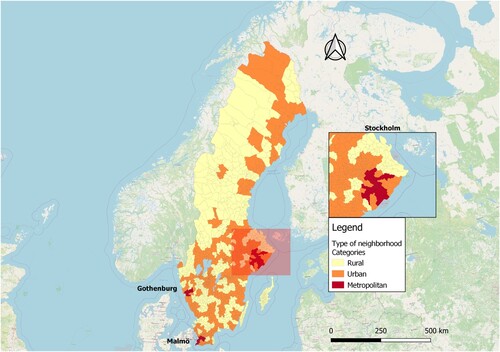
Table 1. Neighbourhood-level distance to the nearest food store, 2000–13.

	All: N = 2511			Rural area: N = 1000			Urban area: N = 1318			Metro area: N = 193
	Mean	Minimum	Maximum	Mean	Minimum	Maximum	Mean	Minimum	Maximum	Mean	Minimum	Maximum
2000
Median distance (km)	3.32	0.00	41.67	3.86	0.00	41.67	3.26	0.25	28.89	0.94	0.00	7.25
Average distance (km)	3.60	0.02	40.73	4.25	0.33	40.73	3.49	0.20	26.21	1.02	0.02	7.02
Average store size (employees)^a	5.44	0.00	100.63	4.51	0.00	208.00	5.37	0.00	155.00	10.84	12.13	104.00
Number of stores	2.12	0.00	36.00	1.21	0.00	14.00	1.95	0.00	34.00	8.05	0.00	36.00
2013
Median distance (km)	3.70	0.00	28.62	4.24	0.00	28.62	3.70	0.25	21.69	0.99	0.00	7.98
Average distance (km)	4.00	0.04	26.93	4.63	0.10	25.97	3.95	0.15	26.93	1.05	0.04	7.61
Average store size (employees)^a	6.81	0.00	100.63	5.48	0.00	89.00	6.72	0.00	202.00	14.20	0.00	126.33
Number of stores	2.04	0.00	35.00	1.08	0.00	13.00	1.84	0.00	26.00	8.42	0.00	35.00

Note: ^aMinimum of 0.00 indicates that there is no store and, hence, zero employees.

N = Observations.

In the year 2000, people living in rural areas had to travel an average of 4.25 km to the nearest food store, people residing in urban areas had to travel 3.5 km, and people in metropolitan areas faced a distance of 1 km. The average store size was similar in urban and rural areas, with approximately five employees, while it was twice that – 11 employees – in the metropolitan areas. People living in rural neighbourhoods had, on average, one store in their neighbourhood, residents in urban neighbourhoods had two stores, and residents in metropolitan neighbourhoods had eight stores.

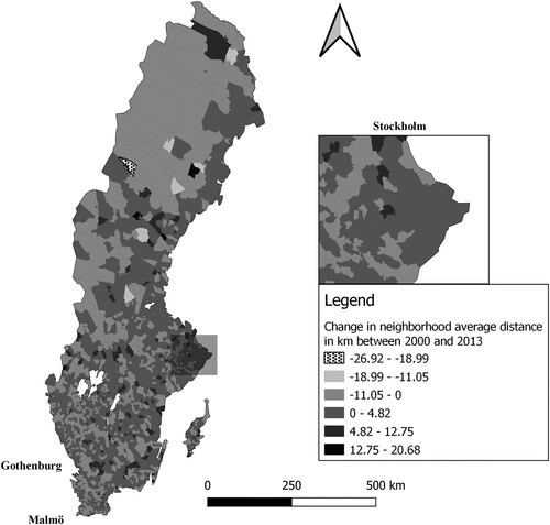
Between 2000 and 2013, the total number of stores in Sweden decreased by 600 – from 5838 to 5238. In this period there was an increase in the population’s distance to the nearest food store by 30–400 m in metropolitan areas, urban areas and rural neighbourhoods (Figure 2). Thus, the increase was of a relatively marginal size, and the internal relationship between the three categories of neighbourhoods remained largely the same. In contrast, the maximum distance to the nearest food store decreased substantially for the inhabitants in rural areas, from 41 to 26 km. At closer inspection of the data, this change is revealed to be driven by an outlier, thus it cannot be considered a general development trend. The drop in the number of stores per neighbourhood type and the increase in the average store size show that stores have become somewhat fewer and larger in both rural and urban areas, indicating economies of scale. However, as the average distances from the population to the stores have not increased much, this also means that the population has become more concentrated in space. In the metropolitan areas, however, the number of stores has increased somewhat.

Figure 2. Change in neighbourhood average distance (km), 2000–13.

Source: Statistics Sweden. Programme: QGIS.

4.1. For whom has the distance changed?

In the literature on food store access, it is argued that a long distance from the nearest food store is especially problematic for individuals who are already facing additional mobility barriers (Ver Ploeg et al., 2009). To capture groups that are vulnerable to poor physical access to groceries, I therefore include variables that show low income, low employment, single-parent households and groups of people aged older than 80 years, measured in 2013. Low-income earners are measured as the share of the neighbourhood population that has an income that is below 50% of the national median worker’s income. Since the data do not allow us to measure unemployment, I use the employment rate, defined as the neighbourhood population between the ages of 20 and 74 that is registered as employed. The share of single-parent households is proxied by the share of the population without a registered partner and with at least one child under 18 years of age living at home. The share of the population over 80 years of age is self-explanatory. The neighbourhoods are categorized based on the size of the changes in the inhabitants’ distance to the nearest store.

Table 2 shows that the population in the neighbourhoods that experienced the largest increases in average distance to the nearest food store (greater than 10 km) and had a higher employment rate (69%) than did the population in the areas that experienced the largest decrease in average distance (64%). The share of low-income earners in the population in the neighbourhoods that experienced the largest decrease in average distance was 38% compared with 31% in the areas with the largest increase. The same is true for the share of people over the age of 80, where the relationship was 10% versus 9%.

Table 2. Characteristics of neighbourhoods with different changes in average distance (right) and different deciles (left).

	Mean shares/changes in distance
Groups	Mean shares (2013) for different distance intervals						Mean distances and changes for different percentiles
	Decreased > 10 km	Decreased 5–10 km	Decreased 0.4–5 km	Increased 0.4–5 km	Increased 5–10 km	Increased > 10 km	Upper (p90) /lower (p10) deciles	Distance (km) (2013)	Change in distance (km) (2000–13)
Share of people > 80 years old	0.10 (0.02)	0.07 (0.04)	0.06 (0.03)	0.06 (0.03)	0.07 (0.03)	0.09 (0.03)	p90	3.49 (3.68)	+0.26 (2.84)
							P10	4.20 (2.54)	+0.14 (1.33)
Share of employed people	0.64 (0.07)	0.70 (0.09)	0.74 (0.06)	0.74 (0.06)	0.71 (0.07)	0.69 (0.06)	p90	5.79 (2.73)	+0.43 (1.89)
							P10	3.25 (4.54)	−0.01 (3.97)
Share of single parents	0.03 (0.02)	0.03 (0.02)	0.03 (0.01)	0.03 (0.01)	0.03 (0.01)	0.04 (0.01)	p90	4.18 (3.19)	+0.47 (2.95)
							P10	6.31 (3.30)	+0.56 (3.10)
Share of low-income earners	0.38 (0.05)	0.33 (0.07)	0.28 (0.05)	0.29 (0.04)	0.31 (0.06)	0.31 (0.05)	P90	5.12 (3.67)	+0.60 (3.13)
							P10	3.58 (2.62)	+0.28 (1.44)
Observations	14	35	286	613	89	15	Obs.	251	251

Note: Standard deviations are shown in parentheses. Obs., observations.

The share of single parents was 3% in the areas with the largest increases in distance and 4% in the areas with the largest decreases in distance. The neighbourhoods whose population experienced decreases in distance, that is, −5 to −10 km versus +5 to +10 km, were relatively similar. However, the neighbourhoods where the population had experienced an increase in the distance to the nearest food store were socio-economically less disadvantaged compared with those that experienced a decrease in distance. Regarding changes of −0.4 to −5 km versus +0.4 to +5 km, the socio-economic characteristics were similar. This indicates that neighbourhoods where the distance increased were similar to those where the distance decreased in terms of socio-economic characteristics. If anything, it was the less socio-economically disadvantaged areas that experienced an increase.

As a last step, the neighbourhoods with the lowest and highest deciles of the socio-economic variables in 2013 are compared in terms of the sizes of the changes in distance between 2000 and 2013. The right part of Table 2 shows that for the share of low-income earners, the most socio-economically disadvantaged areas face a longer distance (1.5 km) to the nearest food store than the less disadvantaged areas. The opposite holds for the areas in the top decile of the shares of individuals over the age of 80, single parents and employed people (the bottom decile for the latter), which have a shorter distance to the nearest food store. In general, the areas with the top deciles of socio-economically disadvantaged groups over 80 years old and low-income earners have seen a larger increase in the distance to the nearest food store than their counterparts. However, the magnitude of the differences is between 100 and 300 m; thus, the magnitude of the differences must be viewed as marginal.

5. EMPIRICAL DESIGN

To examine how changes in population density may explain the development of food store access over time, the spatial and temporal dynamics of the change in food store access are modelled. To limit the changes in the dependent variable to those in the store location, I use the distance from the neighbourhood midpoint, the centroid, to the nearest food store, $d_{nt}^G$.

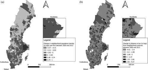
First, let us visually examine the changes in the two main variables: population density and distance (both in natural logarithms) (Figure 3). As expected, population density has increased primarily in the metropolitan and urban neighbourhoods and decreased in the rural neighbourhoods. Regarding the change in distance, the pattern is less striking. There is a weak indication that there has been an increase in distance primarily in the rural areas, however, a statistical analysis is needed to verify this.

A generalized formulation of equation (2)(2) $\mathrm{l}\mathrm{n}{D}_{}={\displaystyle \frac{1}{2}\left(\mathrm{l}\mathrm{n}F-\mathrm{l}\mathrm{n}t-\mathrm{l}\mathrm{n}\rho \right)}$(2) is presented below: (5) $D_{nt}=f\left(F_{nt},t_{nt},{\rho }_{nt}\right)+g\left(\mathit{X}\right)$(5) where $D_{nt}$ is proxied by $ln.d_{nt}^G$, the natural log of the distance from the centroid of each neighbourhood to the nearest food store, in neighbourhood n, at year t. The fixed costs, $F_{nt}$, can be proxied by the neighbourhood-level natural log of average income, $\mathrm{l}\mathrm{n}.ave.in{c}_{nt}$, as a higher level of income in an area, may be correlated with a higher rent (e.g., Van Nieuwerburgh & Weill, 2010). This may have a positive association with $\mathrm{l}\mathrm{n}.d_{nt}^G$ since lower order goods retailers have a lower ability to pay a higher rent, as argued by Garner (1966) and shown by Des Rosiers et al. (2009). It may, however, also be negatively associated with $\mathrm{l}\mathrm{n}.d_{nt}^G$, since a higher income indicates higher purchasing power. A negative correlation is also suggested by the findings of Cleary et al. (2018). Hence, a higher average income may attract food retail stores to an area, thus making the distance to the nearest food store smaller.

Consumer density, ${\rho }_{nt}$, is proxied by the natural log of population density/km² in each neighbourhood. According to the theoretical model, this variable is expected to have a negative correlation with distance to the nearest food store. This is also supported by the empirical literature on access to food stores (e.g., Amin et al., 2020). Based on the theory of economies of scale and previous research (e.g., Parr & Denike, 1970), this association is expected to be negative and non-linear, which is captured by its functional form. $\mathit{X}$ is a vector with two additional variables. The first is the share of families with children in the area, which captures demographic composition to account for the fact that neighbourhoods may have a similar income profile but still differ in terms of demand, hence making the area more or less attractive for a certain type of retail. Lundberg and Lundberg (2010) find that Swedish household expenditures on groceries are positively correlated with the number of individuals in a household that are below 19 years of age. Thus, the share of households with children at home should capture a higher demand for food retail, which should attract food stores to the area, and therefore this variable should have a negative correlation with the dependent variable.

One of the longstanding critiques of the assumptions of CPT is that individuals do not shop at the store that is closest to their homes but in concurrence with other activities, such as travelling to and from work (Fingleton, 1975). Previous studies (Nilsson et al., 2015) have found that around half of grocery shopping trips in Sweden are trip chained with over a third being chained with work trips. To account for the possibility that this may influence store location, the second variable included in $\mathit{X}$ is a variable that captures daytime population density. This is included as the natural log of the density per square kilometre of the number of people who work in the neighbourhood.

Many studies of the determinants of retail location (e.g., Chakraborty, 2012) also include the level of unemployment and level of education of the population. However, these are not included in the present analysis since much of their association with the dependent variable is expected to go through the income variable. The transport costs, t, may vary substantially over the Swedish population, which makes it an important determinant of store location. This variable is difficult to capture with the data available. However, variations in costs over time should be captured by inclusion of time dummies, and variation across space is likely to change slowly over time, and thus, the use of neighbourhood fixed effects (FE) can be expected to alleviate the problem.

According to CPT, the size of a market is correlated with the number and order of retail functions of the market. Thus, the size of a market is indirectly correlated with its relative place in the CPT hierarchy, and therefore, a change in market size, such as population density, may be correlated with a change in the number and order of the functions in other central places. A Pesaran (2004) cross-sectional dependence (CD) test² indicates that there is indeed a significant cross-sectional dependence between the neighbourhoods. Based on theory and the CD test, a model that accounts for global spillovers is justified. To determine which, I follow the ‘classic’ stepwise approach as defined by Burridge (1980) and Anselin (1988) and recommended by Florax et al. (2003), which indicates that the preferred specification is a spatial autoregressive model (SAR), where a spatial lag of the dependent variable is included.³ While the use of a distance-based access variable is beneficial, as it disregards the borders of the areal unit, it has the drawback of not taking competition into account (e.g., Apparicio et al., 2007) as opposed to density measures. However, the SAR model incorporates not only local access but also neighbouring regions’ access, and thus, it captures competition from food stores in other neighbourhoods. Furthermore, the model is estimated with two-way FE,⁴ which prevents time-invariant characteristics, such as natural barriers, from driving the results.

The specification can be expressed as follows: (6) $\begin{array}{rl}\mathrm{l}\mathrm{n}.d_{nt}^G=& \lambda {\mathit{W}}_{}\mathrm{l}\mathrm{n}.d_{jt}^G+{\text{β}}_1\mathrm{l}\mathrm{n}\left(averageincom{e}_{nt}\right)\\ & +{\text{β}}_{2}shareoffamilieswithchildre{n}_{nt}\\ & +{\text{β}}_3\mathrm{l}\mathrm{n}\left(populationdensit{y}_{nt}\right)\\ & +{\text{β}}_4\ln \left(daypopulationdensit{y}_{nt}\right)\\ & +yea{r}_t+a_n+{ϵ}_{nt}\end{array}$(6) where $\lambda$ is the coefficient of the spatially lagged dependent variable, ${\mathit{W}}_{}$is a row-normalized ‘Queen’ contiguity spatial weights matrix,⁵ ${\text{β}}_1$–${\text{β}}_4$ are the coefficients of the explanatory variables, and ${ϵ}_{nt}$ is an error term with an expected mean of zero and a constant variance. Lastly, the model has neighbourhood- and time-specific FEs, denoted $a_n$ and $yea{r}_t$, respectively. The spatial model was fitted using the STATA package xsmle (Belotti et al., 2017), and the model was estimated by the two-step maximum likelihood method. The estimation is run as a non-spatial FE model, and in its spatially augmented form, SAR. For descriptive statistics of the included variables, see Table B2 in Appendix B in the supplemental data online.

6. RESULTS

Table 3 presents the results from the regression model in non-spatial form (FE) and spatial form (SAR). When examining the first column, the FE estimation contains only the main variable of interest, population density, and the coefficient 0.21 of population density is significant and negatively correlated with the distance from the centroid to the nearest food store. Due to the logarithmic transformation of the dependent variable this coefficient can be interpreted as an elasticity, thus, a 1% increase in population density decreases the distance to the nearest food store by 0.21%. The relationship is negative and significant and indicates that an increased demand density decreases the threshold distance, that is, the required market size for a firm to break even. This is in line with CPT and the expectations from the model, as well as with findings of previous studies (e.g., Amin et al., 2020).

Table 3. Regression output.

	Dependent variable: Distance to the nearest food store
Independent variable	ln(centroid-distance to the nearest food store in km), $\mathrm{l}\mathrm{n}\left(d_{jt}^G\right)$					Centroid-distance to the nearest food store in km, $d_{jt}^G$
	(1) FE	(2) FE	(3) TE^b	(4) DE^b	(5) IE^b	(6) FE	(7) TE^b	(8) DE^b	(9) IE^b
ln(population density)	−0.210***	−0.177***	−0.177*	−0.173*	−0.00447
	(0.087)	(0.087)	(0.0914)	(0.0892)	(0.029)
ln(average income)		0.154**	0.165**	0.161**	0.00430	0.334	0.346	0.336	0.0113
		(0.076)	(0.074)	(0.0723)	(0.00272)	(0.443)	(0.444)	(0.433)	(0.0164)
share families with children		−0.382***	−0.391***	−0.381**	−0.00999**	−1.682***	−1.708***	−1.651***	−0.0505*
		(0.109)	(0.108)	(0.106)	(0.004)	(0.608)	(0.611)	(0.594)	(0.0303)
ln(day population density)		−0.011	−0.0112	−0.0114	−0.000293	−0.105*	−0.107*	−0.105	−0.00312
		(0.010)	(0.0103)	(0.010)	(0.0002)	(0.0550)	(0.0552)	(0.0538)	(0.00218)
population density						−0.00574***	−0.00598***	−0.00567**	−0.00017*
						(0.00218)	(0.00230)	(0.00224)	(9.77E–05)
population density*urban^a						0.00392*	0.00411*	0.00399*	(0.000120)
						(0.00208)	(0.00220)	(0.00214)	(8.77E–05)
population density*metro^a						0.00548**	0.00572**	0.00556**	0.000167
						(0.00216)	(0.00227)	(0.00220)	(1.03E–04)
${\mathit{W}}_{}\mathrm{l}\mathrm{n}\left(d_{jt}^G\right)$			0.0256***
${\mathit{W}}_{}{d}_{jt}^G$							0.0290***
LME	47.044***	9.068***				11.934***
RLME	77.444***	12.28***				17.327***
LML	48.585***	10.522***				13.564***
RLML	78.985***	13.734***				18.958***
Global PCD test	913.39***	858.25***				1089.9***
R^2 within	0.015	0.016	0.014			0.0114	0.082
BIC	20,829.32	20,817.9	20,694			134,417.1	134,290.4
AIC	20,710.77	20,673.95	20,643.2			134,256.2	134,222.7
N	35,154	35,154	35,154	35,154	35,154	35,154	35,154	35,154	35,154

Note: ^aThe reference category is a rural neighbourhood.

^b Robust to the W-matrix with three, four and six nearest neighbours. Included but not reported: time- and neighbourhood FE.

FE, fixed effects; SAR, spatial autoregressive regression/or spatial lag-model; DE, direct effects; IE, indirect effects; TE, total effects.

***, ** and *Significant at 1%, 5% and 10%, respectively. Heteroscedasticity and serial correlation robust standard errors are shown in parentheses (Newey & West, 1986; White, 1980).

When the other variables are added, the magnitude of the coefficient decreases to 0.180, but it remains significant and negative. The correlation between average income and the distance from the centroid to the nearest food store is in this model positive and significant with an elasticity of 0.154%, which indicates that food stores may be deterred by locating in areas with higher average income, as these may have higher land rents. This supports previous findings by, for instance, Chakraborty (2012).

The demographic composition, in terms of the share of households with children, is significant and negatively correlated with the distance to the nearest food store, with a coefficient of 0.382. The direction of this correlation is in line with the findings of Lundberg and Lundberg (2010). Lastly, the variable that captures the density of the daytime population is added, and there is no significant effect of this variable.

Turning to the spatial model, one can first observe that the coefficient of the lagged dependent variable, ${\mathit{W}}_{}ln.d_{jt}^G$, is significant and positive. This means that there is a clustering of the values of the dependent variable. Thus, neighbourhoods that have a shorter distance to the nearest food store are likely to be located close to other neighbourhoods that also have a shorter distance to the nearest food store.

The first results of the SAR model (not reported here) cannot be interpreted in the same manner as the partial derivatives in the non-spatial FE model discussed above. The results of the spatial effects are therefore recalculated into three types of marginal effects. Direct effects (DE) are the effects of a change in an independent variable in neighbourhood n on the dependent variable in the same neighbourhood. Conversely, indirect effects (IE) are the effects that a change in an independent variable in n has on the dependent variable in the adjacent neighbourhood, j. The latter may be interpreted as spillover effects. The total effects (TE) is the sum of the DE and IE and thus represents the average effects on the dependent variable. As the relationship between the dependent and independent variables most likely is endogenous, the use of the word ‘effects’ in the text does not indicate causality.

When examining the marginal effects of the SAR estimation (columns 3–5), we find that population density has a direct correlation of −0.177 and an indirect correlation of −0.00447 with the distance to the nearest food store. Thus, a 1% increase in the population density in neighbourhood n is correlated with a decrease of 0.177% in the distance to the nearest food store in neighbourhood n and a minor decrease in adjacent neighbourhood j. The spillover effect is not significant; however, one can deduce that the influence of a change in population density on distance consists of direct effects.

In the spatial model, income has a total positive effect on the distance to the nearest food store, which is of a similar magnitude to the result in the non-spatial model. The share of families with children is negatively correlated with distance to the nearest food store, with a minor significant negative spillover effect on adjacent neighbourhoods.

The daytime population density variable was insignificant in the non-spatial model and remained so in the spatial model.⁶ Hence, the change in distance to the nearest food store appears to be correlated primarily with residential population density, demographic composition, and average income.

To assess how the correlation between population density and distance varies depending on the type of region in which the neighbourhood is in, I estimate the model again, but now I interact population density with dummy variables indicating whether the neighbourhood is located in a rural, urban or metropolitan municipality. Since the non-linearity will now be captured by the interaction between population density and the different dummy variables, I include population density and the interactions in levels.⁷ The dependent variable also enters in levels, while the other explanatory variables are included in their previous functional form. The type of neighbourhood is determined by the classification of its municipality, and is time-invariant, hence, in the FE framework the main terms of the categories will not generate any coefficients. While it is possible for a municipality to change classification, the broad definitions (three levels), and large areal units (290 municipalities in Sweden) and a relatively short period of time, makes this unlikely.

As seen in column 6, the correlation between population density and the distance to the nearest food store is negative in its main effect. The coefficient of the interaction between population density and the urban dummy is positive, 0.00392. Thus, compared with the reference category, which is rural, population density has a positive correlation with distance to the nearest food store. The coefficient for the interaction with the metropolitan dummy is also positive and somewhat larger, 0.00548. This means that an increase in population density is correlated with a decrease in the distance to the nearest food store at a rate that is the highest in rural neighbourhoods, followed by urban neighbourhoods and at the lowest rate in metropolitan neighbourhoods. This indicates that as population density has declined, access to food stores has decreased at the highest rate in rural areas and at the lowest rate in metropolitan areas. Thus, in more densely populated areas, the effect of population density is less pronounced (less negative), which suggests the presence of decreasing returns to size of demand. However, as noted earlier, the number of stores had increased in metropolitan neighbourhoods, thus, the low rate of decline in access here could also be due to a fragmentation of larger stores into relatively smaller formats, which is a trend connected to the increase in omnichannel retailing (Gauri et al., 2021).

When examining the results from the spatial model, the size of the total effects is similar to that of the non-spatial model, and as before, the chief part of the effect consists of the direct effects.

6.1. Robustness tests

The choice of parishes as the spatial unit may be subject to the modifiable areal unit problem (MAUP) (Openshaw, 1981), and hence, the relationship between population density and distance to the nearest food store may be due to aggregation. To address this, I created an unbalanced panel dataset based on 5×5 km sized grids on which I estimated the model in equation (5)(5) $D_{nt}=f\left(F_{nt},t_{nt},{\rho }_{nt}\right)+g\left(\mathit{X}\right)$(5) again. The results in Table C1 in column 1 in Appendix C in the supplemental data online show that the relationship between population density and distance holds in terms of significance and direction. The magnitude of the coefficient is considerably smaller, however, but since the number of grids is considerably larger than the number of parishes (there are approximately 85,000 grids and 2500 parishes), this is expected. In column 2 of Table C1, the interaction effect between the type of municipality in which the grid is located shows a similar relationship between metro and urban and the baseline category, rural. Hence, the main results remain robust to an alternative shape and size of the areal unit.

As noted in Figure 3, many but not all of the declining regions (in terms of population growth) have seen a decrease in food store access. This may imply that the process of store location differs between growing and declining regions. The dataset was therefore split into neighbourhoods that had experienced a net increase in population density between 2000 and 2013 and neighbourhoods that had experienced a net decrease, and the non-spatial FE estimation of equation (6)(6) $\begin{array}{rl}\mathrm{l}\mathrm{n}.d_{nt}^G=& \lambda {\mathit{W}}_{}\mathrm{l}\mathrm{n}.d_{jt}^G+{\text{β}}_1\mathrm{l}\mathrm{n}\left(averageincom{e}_{nt}\right)\\ & +{\text{β}}_{2}shareoffamilieswithchildre{n}_{nt}\\ & +{\text{β}}_3\mathrm{l}\mathrm{n}\left(populationdensit{y}_{nt}\right)\\ & +{\text{β}}_4\ln \left(daypopulationdensit{y}_{nt}\right)\\ & +yea{r}_t+a_n+{ϵ}_{nt}\end{array}$(6) was repeated. The results from the estimation (see Table D1, column 1, in Appendix D in the supplemental data online) showed that the coefficient of population density remained significant, of the same sign, and of a similar magnitude (with an elasticity of −0.22%) in the growing regions, while this was not the case in the sample with declining regions. Thus, the relationship between store access and density does not hold for the declining regions. As argued by Melitz and Trefler (2012) a firm may wait to exit until its fixed capital has depreciated; thus, there may be more pronounced inertia in exits of (food) stores than in entries. As reported in SOU (2015), there is, in some instances, also support from local volunteers in running the grocery stores in areas with declining populations, and this could contribute to the resilience of these stores. Moreover, as declining regions have also been the targets of subsidies, the exit or relocation of food stores out of a market could be delayed even further. In subsequent estimations (results are available upon request), time lags of population density were included, but with no significant results. It is likely that the current dataset has a too short time period for investigating any potential long run effects of population decline.

Figure 3. (a) Change in neighbourhood population density/km² (in natural logarithms), 2000–13; and (b) change in distance from neighbourhood centroids to the nearest food store (km) (in natural logarithms), 2000–13.

Source: Statistics Sweden. Programme: QGIS.

In the assessment of how the relationship varied by degree of centrality in the growing regions, the initial results remained significant and of similar magnitude and had the same sign for metropolitan and rural areas, while the coefficient for urban became insignificant (see Table D1, column 2, in Appendix D in the supplemental data online). The coefficient of urban did, however, retain the same sign and a similar magnitude. Since the relationship between density and store access is significant only in the growing region subsample, this suggests that the results of the analysis of the effects of density by degree of centrality in the complete dataset are driven by the growing regions. Thus, in the analysis of the growing region subsample, the reason that the difference between urban and rural regions is insignificant is likely due to the use of a smaller dataset in combination with a relatively low level of within-variation and the multicollinearity that stems from the interaction terms.

7. CONCLUSIONS AND POLICY IMPLICATIONS

The findings from the descriptive analysis show that there has been an increase in distance to the nearest food store. However, it seems that it is primarily the socio-economically advantaged groups that have experienced an increase, and hence a decline in access; thus, the findings are in line with those of Amcoff (2017). Furthermore, the largest increases in distance were found in rural areas, and hence, the groups and areas where measures of intervention are needed most urgently are in neighbourhoods that are characterized by higher socio-economic status and rural places.

The results from the regression analysis show that population density is negatively correlated with distance to the nearest food store, a relationship that is most pronounced in rural neighbourhoods. However, when assessing the growing and declining regions separately, I find that the results do not hold for the declining regions but are driven by the growing regions. It is not possible to deduce a causal effect of population density, as regional growth is a complex process, and there may be underlying trends that drive both population growth and location of grocery stores. However, these findings suggest that a denser spatial configuration of housing is preferred in growing regions to increase access to groceries, while the (zero) results for the declining regions could have several implications. They may imply that the process of store exit is one that takes place over several years and that it is therefore not possible to capture this process using the current data set. It could also mean that efforts – from local volunteers and in the form of financial support – may, to some extent, have delayed firm exits. The results in this study hold for the period 2000–13, which was the same period that subsidies (of tens of millions of US$) from the EU and the Swedish government have been focused on maintaining access to basic commercial services in places with declining populations. While it is not feasible in this study to deduce whether the subsidies had an effect, the fact that the declines in some regions were not significantly correlated with a decrease in store access could imply that the subsidies may have prolonged the lives of grocery stores in those areas. Thus, there is a need for future research to assess to what extent, if any, the subsidies have had an impact on ensuring access to basic commercial services such as food stores.

Regardless of the correlation between population density and store access, the descriptive analysis showed that there has been a decline in physical access to food stores. It may be argued that, due to spatial sorting of residents into areas where their preferences in terms of food stores are met, the decline in access is not a market failure. However, due to the heavily regulated Swedish rental market, with artificially low rents, and highly inflated housing prices, there has for the past 20 years been a consistent deficit in the supply of housing, particularly in amenity-rich areas. Therefore, the spatial sorting of individuals from amenity-poor to amenity-rich areas is limited, which implies that the development may in fact be suboptimal from a social welfare perspective.

To what extent can we hope for digital solutions? Online grocery retailing has grown dramatically in the past decade. Between 2014 and 2019, it grew on average by 28% annually (The Swedish Trade Federation, 2020), and between 2019 and 2020, it even doubled. However, online grocery sales as a share of total grocery sales remains at a more modest level, amounting to a mere 4% of total grocery sales in 2020 (PostNord, 2021). One of the reasons behind this low figure is believed to be the high last-mile costs in rural areas, which limits home delivery to urban and metropolitan areas. Alternative solutions, such as click-and-collect⁸ have a somewhat greater reach but they are also reserved for urban areas. Moreover, online solutions precondition an adequate coverage in broadband and mobile connections, and these still remain insufficient in many rural areas in Sweden (Swedish Agency for Growth Policy Analysis, 2021). Hence, a transition to online grocery retailing is not possible for all parts of the population, and for them the distance to a food store is still of high relevance.

ACKNOWLEDGEMENTS

The author thanks Mikaela Backman, Emek Basker, Sven-Olov Daunfeldt, Johannes Hagen, Johan Klaesson, Sierdjan Koster, Johan P. Larsson, Agostino Manduchi, Giovanni Millo, Pia Nilsson, Paul Nystedt, Andrés Rodríguez-Pose and Özge Öner; as well as the participants at: the HUI Workshop on Research in Retailing, 2018; European Regional Science Conference, 2018 and 2019; and the anonymous reviewers for valuable comments that have significantly improved the quality of this paper.

DISCLOSURE STATEMENT

No potential conflict of interest was reported by the author .

Additional information

Funding

Research funding (in the form of scholarships) from the Swedish Retail and Wholesale Council (Handelsrådet) and the Institute of Retail Economics (Handelns Forskningsinstitut) is gratefully acknowledged.

Notes

1. Definitions from The Swedish Agency for Growth Policy Analysis (2014), based on data from 2007 to 2010.

2. The CD test was conducted using the plm package (Millo & Croissant, 2008).

3. This model was also indicated by the test of Anselin et al. (1996), which allows for panel structure and within effects.

4. The Hausman test also indicates neighborhood specific FE.

5. The specification is robust to alternative spatial weight matrix specifications the of three, four and six nearest neighbours.

6. As a robustness test, population density was replaced by day population density; however, the results (available from the author upon request) did not change.

7. This is because a 1% change in population density in a rural area will not be the same as a 1% change in an urban area. Thus, to assess whether there are any differences across region types, population density enters the regression in levels.

8. ‘Click and collect’ implies that goods are ordered online and collected by the consumer at the nearest food store or a service point.

REFERENCES

- Allcott, H., Diamond, R., Dubé, J.-P., Handbury, J., Rahkovsky, I., & Schnell, M. (2019). Food deserts and the causes of nutritional inequality. The Quarterly Journal of Economics, 134(4), 1793–1844. https://doi.org/10.1093/qje/qjz015
- Amcoff, J. (2017). Food deserts in Sweden? Access to food retail in 1998 and 2008. Geografiska Annaler: Series B, Human Geography, 99(1), 94–105. https://doi.org/10.1080/04353684.2016.1277076
- Amin, M. D., Badruddoza, S., & McCluskey, J. J. (2020). Predicting access to healthful food retailers with machine learning. Food Policy, 101985, https://doi.org/10.1016/j.foodpol.2020.101985
- Anselin, L. (1988). Lagrange multiplier test diagnostics for spatial dependence and spatial heterogeneity. Geographical Analysis, 20(1), 1–17. https://doi.org/10.1111/j.1538-4632.1988.tb00159.x
- Anselin, L., Bera, A. K., Florax, R. J. G. M., & Yoon, M. J. (1996). Simple diagnostic tests for spatial dependence. Regional Science and Urban Economics, 26(1), 77–104. https://doi.org/10.1016/0166-0462(95)02111-6
- Apparicio, P., Abdelmajid, M., Riva, M., & Shearmur, R. (2008). Comparing alternative approaches to measuring the geographical accessibility of urban health services: Distance types and aggregation-error issues. International Journal of Health Geographics, 7(1), 1–14. https://doi.org/10.1186/1476-072X-7-7
- Apparicio, P., Cloutier, M.-S., & Shearmur, R. (2007). The case of Montreal's missing food deserts: Evaluation of accessibility to food supermarkets. International Journal of Health Geographics, 6(1), 1–13. https://doi.org/10.1186/1476-072X-6-4
- Belotti, F., Hughes, G., & Mortari, A. P. (2017). Spatial panel-data models using Stata. The Stata Journal, 17(1), 139–180. https://doi.org/10.1177/1536867X1701700109
- Berry, B. J. L., & Garrison, W. L. (1958). A note on central place theory and the range of a good. Economic Geography, 34(4), 304–311. https://doi.org/10.2307/142348
- Biagi, B., Faggian, A., & McCann, P. (2011). Long and short distance migration in Italy: The role of economic, social and environmental characteristics. Spatial Economic Analysis, 6(1), 111–131. https://doi.org/10.1080/17421772.2010.540035
- Burridge, P. (1980). On the cliff-Ord test for spatial correlation. Journal of the Royal Statistical Society: Series B, 42(1), 107–108. https://doi.org/10.1111/j.2517-6161.1980.tb01108.x
- Chakraborty, K. (2012). Estimation of minimum market threshold for retail commercial sectors. International Advances in Economic Research, 18(3), 271–286. https://doi.org/10.1007/s11294-012-9354-3
- Christaller, W. (1966). Central places in southern Germany. Prentice-Hall.
- Clarke, I., & Banga, S. (2010). The economic and social role of small stores: A review of UK evidence. The International Review of Retail, Distribution and Consumer Research, 20(2), 187–215. https://doi.org/10.1080/09593961003701783
- Cleary, R., Bonanno, A., Chenarides, L., & Goetz, S. J. (2018). Store profitability and public policies to improve food access in non-metro US counties. Food Policy, 75, 158–170. https://doi.org/10.1016/j.foodpol.2017.12.004
- Cummins, S., Findlay, A., Higgins, C., Petticrew, M., Sparks, L., & Thomson, H. (2008). Reducing inequalities in health and diet: Findings from a study on the impact of a food retail development. Environment and Planning A, 40(2), 402–422. https://doi.org/10.1068/a38371
- Cummins, S., & Macintyre, S. (2002). A systematic study of an urban foodscape: The price and availability of food in Greater Glasgow. Urban Studies, 39(11), 2115–2130. https://doi.org/10.1080/0042098022000011399
- Dawson, J. (2006). Retail trends in Europe. In Retailing in the 21st century (pp. 41–58). Springer. https://doi.org/10.1007/978-3-540-72003-4_5.
- Des Rosiers, F., Thériault, M., & Lavoie, C. (2009). Retail concentration and shopping center rents –– A comparison of two cities. Journal of Real Estate Research, 31(2), 165–208. https://doi.org/10.1080/10835547.2009.12091250
- Donald, B. (2013). Food retail and access after the crash: Rethinking the food desert problem. Journal of Economic Geography, 13(2), 231–237. https://doi.org/10.1093/jeg/lbs064
- Dutko, P., Ver Ploeg, M., & Farrigan, T. L. (2012). Characteristics and influential factors of food deserts (Report No. 140). United States Department of Agriculture. https://ageconsearch.umn.edu/record/262229/files/30940_err140.pdf. https://doi.org/10.22004/ag.econ.262229.
- Fingleton, B. (1975). A factorial approach to the nearest centre hypothesis. Transactions of the Institute of British Geographers, 65(65), 131–139. https://doi.org/10.2307/621613
- Florax, R. J. G. M., Folmer, H., & Rey, S. J. (2003). Specification searches in spatial econometrics: The relevance of Hendry’s methodology. Regional Science and Urban Economics, 33(5), 557–579. https://doi.org/10.1016/S0166-0462(03)00002-4
- Garner, B. J. (1966). The internal structure of retail nucleations (Publication No. 6411259) [Doctoral Dissertation] Department of Geography, Northwestern University.
- Gauri, D. K., Jindal, R. P., Ratchford, B., Fox, E., Bhatnagar, A., Pandey, A., Navallo, J. R., Fogarty, J., Carr, S., & Howerton, E. (2021). Evolution of retail formats: Past, present, and future. Journal of Retailing, 97(1), 42–61. https://doi.org/10.1016/j.jretai.2020.11.002
- Gordon, C., Purciel-Hill, M., Ghai, N., Kaufman, L., Graham, R., & Van Wye, G. (2011). Measuring food deserts in New York city’s low-income neighborhoods. Health & Place, 17(2), 696–700. https://doi.org/10.1016/j.healthplace.2010.12.012
- Grediaga, I. O., & Freshwater, D. (2010). Strategies to improve rural service delivery. (Rural Policy Reviews) OECD Publishing. https://doi.org/10.1787/9789264083967-en.
- Gutiérrez, J., & García-Palomares, J. C. (2008). Distance-measure impacts on calculation of transport service areas using GIS. Environment and Planning B: Planning and Design, 35(3), 480–503. https://doi.org/10.1068/b33043
- Hamidi, S. (2020). Urban sprawl and the emergence of food deserts in the USA. Urban Studies, 58(8), 1660–1675. https://doi.org/10.1177/0042098019841540
- Harris, T. R., Chakraborty, K., Xiao, L., & Narayanan, R. (1996). Application of count data procedures to estimate thresholds for rural commercial sectors. Review of Regional Studies, 26(1), 75–88. https://doi.org/10.52324/001c.8957
- Hodge, I., Dunn, J., Monk, S., & Kiddle, C. (2000). An exploration of ‘bundles’ as indicators of rural disadvantage. Environment and Planning A, 32(10), 1869–1887. https://doi.org/10.1068/a32196
- Ilbery, B., & Maye, D. (2006). Retailing local food in the Scottish–English borders: A supply chain perspective. Geoforum; Journal of Physical, Human, and Regional Geosciences, 37(3), 352–367. https://doi.org/10.1016/j.geoforum.2005.09.003
- Isard, W. (1956). Location and space-economy. Wiley.
- Larson, N. I., Story, M. T., & Nelson, M. C. (2009). Neighborhood environments: Disparities in access to healthy foods in the US. American Journal of Preventive Medicine, 36(1), 74–81.e10. https://doi.org/10.1016/j.amepre.2008.09.025
- Losch, A. (1964). Economics of location. Yale University.
- Lundberg, J., & Lundberg, S. (2010). Retailer choice and loyalty schemes – evidence from Sweden. Letters in Spatial Resource Sciences, 3(3), 137–146. https://doi.org/10.1007/s12076-010-0044-6
- Marshall, D., Dawson, J., & Nisbet, L. (2018). Food access in remote rural places: Consumer accounts of food shopping. Regional Studies, 52(1), 133–144. https://doi.org/10.1080/00343404.2016.1275539
- Melitz, M. J., & Trefler, D. (2012). Gains from trade when firms matter. Journal of Economic Perspectives, 26(2), 91–118. https://doi.org/10.1257/jep.26.2.91
- Millo, G., & Croissant, Y. (2008). Panel data econometrics in R: The plm package. Journal of Statistical Software, 27, 2. https://doi.org/10.18637/jss.v027.i02
- Mulligan, G. F., Wallace, M. L., & Plane, D. A. (1985). A general-model for estimating the number of tertiary establishments in communities – An Arizona perspective. Social Science Journal, 22(2), 77–93.
- Mushinski, D., & Weiler, S. (2002). A note on the geographic interdependencies of retail market areas. Journal of Regional Science, 42(1), 75–86. https://doi.org/10.1111/1467-9787.00250
- Newey, W. K., & West, K. D. (1986). A simple, positive semi-definite, heteroskedasticity and autocorrelation consistent covariance matrix (Technical Working Paper No. 55). National Bureau of Economic Research (NBER).
- Nilsson, E., Gärling, T., Marell, A., & Nordvall, A.-C. (2015). Who shops groceries where and how?–the relationship between choice of store format and type of grocery shopping. The International Review of Retail, Distribution and Consumer Research, 25(1), 1–19. https://doi.org/10.1080/09593969.2014.940996
- OECD.Stat. (2020). Regulation in retail trade 2013. https://stats.oecd.org/Index.aspx?DataSetCode=RETAIL.OECD
- OpenStreetMap contributors. (2020). © OpenStreetMap is open data, licensed under the Open Data Commons Open Database License (https://opendatacommons.org/licenses/odbl/) by the OpenStreetMap Foundation (OSMF). URL to copyright: openstreetmap.org/copyright.
- Openshaw, S. (1981). The modifiable areal unit problem. Quantitative geography: A British view, 60–69. GeoBooks.
- Parr, J. B., & Denike, K. G. (1970). Theoretical problems in central place analysis. Economic Geography, 46(4), 568–586. https://doi.org/10.2307/142941
- Pesaran, H. M. (2004). General diagnostic tests for cross-sectional dependence in panels (Working Paper No. 1229). Center for Economic Studies and ifo Institute (CESifo).
- PostNord. (2021). E-barometern årsrapport 2020 [Online retail, annual report, 2020]. https://www.postnord.se/siteassets/pdf/rapporter/e-barometern-arsrapport-2020.pdf
- Powell, L. M., Slater, S., Mirtcheva, D., Bao, Y., & Chaloupka, F. J. (2007). Food store availability and neighborhood characteristics in the United States. Preventive Medicine, 44(3), 189–195. https://doi.org/10.1016/j.ypmed.2006.08.008
- QGIS Development Team. (2020). QGIS (Version 3.16 Hannover). Geographic Information System. Open Source Geospatial Foundation Project. http://qgis.osgeo.org.
- Salop, S. C. (1979). Monopolistic competition with outside goods. The Bell Journal of Economics, 10(1), 141–156. https://doi.org/10.2307/3003323
- Social Exclusion Unit. (1998). Bringing Britain together: A national strategy for neighbourhood renewal (Cm 4045). Stationery Office.
- SOU. (2015). Service i Glesbygd. [Service in rural areas] (Statens offentliga utredningar No. 2015:35). Government of Sweden. https://lagen.nu/sou/2015:35#sid3-text
- The Swedish Agency for Economic and Regional Growth. (2015). Uppdrag att fördela medel för insatser inom området kommersiell service i gles- och landsbygder. Slutrapport. [Assignment to distribute funds for efforts in the area of commercial service in sparse and rural areas. Final report] (No. 0612).
- The Swedish Agency for Growth Policy Analysis. (2014). Bättre statistik för bättre regional- och landsbygdspolitik [Improved statistics for better regional- and rural policies] (No. 2014:4).
- Swedish Agency for Growth Policy Analysis. (2021). Tillgänglighet till komersiell service och offentlig service, 2021 [Availability to commercial and public service, 2021] (No. 0369).
- The Swedish Consumer Agency. (2008). Kommersiell service i alla delar av landet – Redovisning av insatser och erfarenheter 2002–2007 [Commercial service in all parts of the country – Accounting of efforts and experiences 2002–2007]. (No. 2008:06).
- Swedish Parliament. (2000). Förordning (2000:284) om stöd till kommersiell service. [Regulation (2000: 284) on support for commercial service].
- The Swedish Trade Federation. (2020). Läget i Handeln, 2020 års rapport om branschens ekonomiska utveckling [The situation in retail: 2020 Report on the development of the sector] (Läget i Handeln No. 2020).
- Thilmany, D., McKenney, N., Mushinski, D., & Weiler, S. (2005). Beggar-thy-neighbor economic development: A note on the effect of geographic interdependencies in rural retail markets. The Annals of Regional Science, 39(3), 593–605. https://doi.org/10.1007/s00168-005-0229-x
- Turok, I., & Mykhnenko, V. (2007). The trajectories of European cities, 1960–2005. Cities, 24(3), 165–182. https://doi.org/10.1016/j.cities.2007.01.007
- Van Nieuwerburgh, S., & Weill, P.-O. (2010). Why has house price dispersion gone up? The Review of Economic Studies, 77(4), 1567–1606. https://doi.org/10.1111/j.1467-937X.2010.00611.x
- Varela-Candamio, L., Morollón, F. R., & Sedrakyan, G. (2019). Urban sprawl and local fiscal burden: Analysing the Spanish case. Empirica, 46(1), 177–203. https://doi.org/10.1007/s10663-018-9421-y
- Ver Ploeg, M., Breneman, V., Farrigan, T., Hamrick, K., Hopkins, D., Kaufman, P., Lin, B. H., Nord, M., Smith, T. A., Williams, R., & Kinnison, K. (2009). Access to affordable and nutritious food: measuring and understanding food deserts and their consequences: report to congress (Administrative Publications No. 036). United States Department of Agriculture.
- Wensley, M. R. D., & Stabler, J. C. (1998). Demand-threshold estimation for business activities in rural Saskatchewan. Journal of Regional Science, 38(1), 155–177. https://doi.org/10.1111/0022-4146.00086
- White, H. (1980). A heteroskedasticity-consistent covariance matrix estimator and a direct test for heteroskedasticity. Econometrica, 48(4), 817–838. https://doi.org/10.2307/1912934
- Wrigley, N. (2002). ‘Food deserts’ in British cities: Policy context and research priorities. Urban Studies, 39(11), 2029–2040. https://doi.org/10.1080/2F0042098022000011344
- Öner, Ö. (2017). Retail city: The relationship between place attractiveness and accessibility to shops. Spatial Economic Analysis, 12(1), 72–91. https://doi.org/10.1080/17421772.2017.1265663