Optimisation-based coordination of connected, automated vehicles at intersections

ABSTRACT

In this paper, we analyse the performance of a model predictive controller for coordination of connected, automated vehicles at intersections. The problem has combinatorial complexity, and we propose to solve it approximately by using a two stage procedure where (1) the vehicle crossing order in which the vehicles cross the intersection is found by solving a mixed integer quadratic program and (2) the control commands are subsequently found by solving a nonlinear program. We show that the controller is persistently safe and compare its performance against traffic lights and two simpler optimisation-based coordination schemes. The results show that our approach outperforms the considered alternatives in terms of both energy consumption and travel-time delay, especially for medium to high traffic loads.

KEYWORDS:

• Connected and autonomous vehicles
• model predictive control
• intelligent transportation systems

1. Introduction

By combining Autonomous Driving (AD) technologies with communication [1,2], cooperative strategies can be implemented, which augment the capabilities of automated vehicles. In this paper, we consider such a strategy for coordinating connected and automated vehicles (CAV) at intersections, where the traffic system is burdened with high accident rates [3], congestion and energy-waste [4]. Currently, vehicles are coordinated at intersections with combinations of traffic lights, road signs and right-of-way rules, but with the introduction of CAVs, the coordination could instead be automated.

Unfortunately, the design of algorithms and controllers for this application is challenging for several reasons. First, the general problem of finding collision-free trajectories for vehicles crossing intersections has been shown to be NP-hard [5]. Additionally, imperfect prediction models, non-ideal sensors and impairments of the wireless communication channel [6] lead to uncertainties that necessitate closed-loop control. That is, the coordination must be updated repeatedly by accounting for the most up-to-date information from the vehicles. Establishing that such closed-loop systems are stable and persistently safe is in general a difficult task.

1.1. Solving the intersection coordination problem

The problem of coordinating CAVs at intersections has been surveyed in [7,8]. Most existing contributions are focused on scenarios where all vehicles are automated, and disregard non-cooperative entities such as legacy vehicles or pedestrians. A large part of this work has been performed outside the control community and has relied heavily on tailored heuristics [9–11]. However, the problem is naturally formulated as a constrained optimal control problem (OCP), as it involves the optimisation of trajectories generated by dynamical systems, subject to (at least) collision avoidance constraints. A number of contributions have, therefore, been proposed by the control community [12–35]. However, solving the coordination OCP includes finding the order in which the vehicles cross the intersection and the space of possible solutions grows rapidly with the number of vehicles involved. Most existing approaches, therefore, avoid treating the coordination OCP directly, and are often based on a mix of heuristics and simpler OCPs. These schemes can roughly be categorised as Sequential/Parallel or Simultaneous, depending on what type of OCPs they involve.

In Sequential/Parallel schemes, a priority ranking of the vehicles is typically decided first. The solution is thereafter obtained by solving a number of smaller OCPs, commonly one per vehicle, where constraints are imposed to avoid collisions with higher priority vehicles. The ranking itself is typically the result of a heuristic, where common choices are variations of first-come-first-served (FCFS) policies.

In purely Sequential schemes such as [12,13] or the so-called $MP{C}^{\ast }$  [14], the vehicles compute their solution in sequence based on a decision order, which implicitly reflects the priority. That is, each vehicle solves an OCP, constrained to avoid collisions with respect to the (already decided and available) solutions from the OCPs of vehicles preceding it in the decision order.

In Parallel schemes instead, the vehicle OCPs use predictions of higher priority vehicles' trajectories. Along these lines, Kim and Kumar [15] propose to use conservative estimates, based on predicted trajectories resulting from maximum braking manoeuvres. With the so-called $MP{C}_0$ solution, Qian et al. [14] suggest constant velocity predictions, whereas constant acceleration predictions are considered in [16]. Another alternative, suitable for receding horizon implementations, is to use the predicted trajectories of the higher priority vehicles from the previous time instant (see, e.g. [17–20] and the so-called $MP{C}_1$  [14]). If the priority ordering is constant between two time instants, this corresponds to a sequential solution with delayed information exchange. A scheme, which uses both sequential and parallel components, was suggested in [21]. There, a crossing time schedule is first constructed sequentially based on an FCFS policy, followed by the parallel solution of OCPs to compute the state and control trajectories.

Due to the reliance on priority relations, Sequential/Parallel schemes are often ‘greedy’, in the sense that a high priority vehicle does not take decisions that are beneficial to lower priority vehicles, if that decision is detrimental to the high priority vehicle itself. As a consequence, the effort required to resolve difficult conflicts is typically pushed ‘downwards’ in the priority hierarchy. Although sub-optimal by design, these schemes are often suitable for decentralised implementations with low and accurately predictable requirements on computation and information exchange.

In Simultaneous methods, on the other hand, the solution is found through joint optimisation of several vehicles' trajectories. However, to manage the combinatorial complexity, the crossing order parts of the solution are typically still found using heuristics. In most schemes, this is done by first selecting the crossing order using a heuristic (often variations of FCFS policies), and thereafter jointly optimising the trajectories of the vehicles for the given crossing order. Such fixed-order joint optimisation was considered in [24–31]. Alternative approaches (e.g. [32,33]) apply local continuous optimisation methods to the full coordination OCP directly. The crossing order is thus selected by the optimiser, but depends on the initial-guess provided to the solver. A few contributions propose to solve the full coordination OCP directly and simultaneously optimise all aspects of the problem. For instance, both [34] and the benchmark discussed in [35] consider mixed-integer quadratic programming (MIQP) formulations of the problem, returning both the optimal trajectories and crossing order. Although such approaches are able to find optimal solutions, they typically scale poorly with the problem size (i.e. number of vehicles) and are therefore practically limited to small problem instances.

While Simultaneous approaches, in general, optimise over a larger set of solutions than their Sequential/Parallel counterparts, their application is significantly more involved. In particular, since the joint problems must be solved iteratively, the solution is either computed with standard tools in a completely centralised fashion [24–26], or with iterative, distributed optimisation algorithms [27–31] which rely on repeated communication between the vehicles and a central network node. As a result, the computational and communication requirements of Simultaneous approaches are, in general, higher and harder to predict accurately than those of Sequential/Parallel approaches.

1.2. Contribution

In this paper, we evaluate the performance of a closed-loop algorithm directly derived from the full OCP formulation of the intersection problem, where the optimal solution is obtained by joint optimisation of all parts of the problem, but performed in two stages. Similar to most other Simultaneous schemes, we first find the crossing order and thereafter solve a fixed-order OCP for the vehicle trajectories. However, contrary to the methods described above, the crossing order is found by solving an approximate, lower dimensional representation of the full problem in the form of an MIQP, which approximately accounts for the constraints and objective of the full problem. We extend the work of Hult et al. [27,36–39], by introducing the possibility to add and remove vehicles from the intersection scenario, thus simulating the arrival of new vehicles and the departures of vehicles which have already crossed the intersection. Since our approach is applicable to a vast class of vehicle models, we first present it in a general form, and afterwards we compare it to other approaches on a specific example in simulations.

We evaluate the closed-loop performance of the receding horizon application of the controller on a simulated scenario and compare it with the performance of (1) an overpass solution where the roads are physically separated, (2) a traffic light controller, (3) a controller based on the sequential solution of OCPs, and (4) a controller where the crossing order is obtained through a first-come-first-serve heuristic and the trajectories are jointly optimised. The purpose of the comparisons is to establish (1) the loss induced by the proposed controller with respect to the overpass solution, (2) the gain with respect to the traffic light controller, and (3) the performance difference between the cases where nothing is optimised jointly, where only the trajectories are optimised jointly or where both the trajectories and the crossing order are optimised jointly.

The remainder of the paper is organised as follows: in Section 2, we introduce the proposed coordination algorithm. In Section 3, we introduce the scenario on which we evaluate the performance and detail the benchmarks considered. We discuss the results in Section 4 and conclude the paper in Section 5.

2. Optimal coordination at intersections

In this section, we model the intersection scenario and introduce the two-stage approximation procedure. Both the scenario modelling and the problem formulation are based on the following fundamental assumption.

Assumption 2.1

No non-cooperative entities are present in the scenario.

That is, we do not consider scenarios with, for example, legacy vehicles, pedestrians or bicyclists. Assumption 2.1, though standard in the literature on vehicle coordination problems, see, e.g. [11,12,21,40,41], is restrictive and may limit the applicability of coordination algorithms. We remark that our approach can be extended to accommodate the presence of non-cooperative road users by introducing appropriate models describing their behaviour in traffic. This is the subject of ongoing research.

Under these assumptions, the coordination problem is informally stated as ‘Find the control commands for all CAVs in the vincinity of the intersection which result in collision-free state trajectories that are consistent with the vehicle dynamics, satisfy all physical and design constraints and maximise performance.’

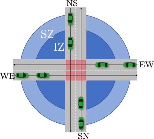
For ease of presentation and interpretation of the results, we consider only scenarios like the one shown in Figure 1(a), with two intersecting single-lane roads, where no turns are allowed. We remark that the formalism presented in this paper can be applied to more general settings including multiple lanes [37] and turning vehicles [39].

Figure 1. Illustrations of collision avoidance conditions. (a) Illustration of Assumption 2.2 and the Conflict Zones (red boxes); (b) scheme of the SICA condition (3(3) $(x_i(t),x_j(t))\notin {\hat{\mathcal{B}}}_{r,ij}=\{(x_i,x_j)|p_i\in [p_{r,i}^{\mathrm{in}},p_{r,i}^{\mathrm{out}}],p_j\in [p_{r,j}^{\mathrm{in}},p_{r,j}^{\mathrm{out}}]\},$(3) ): ${\hat{\mathcal{G}}}_i(p_i(t))$ shown as boxes around the vehicles and (c) conservativeness induced by rectangular outer approximations.

2.1. Scenario modeling

While one can model the motion of the CAVs in the intersection with arbitrary accuracy, the following assumption, widely accepted in the literature [12,14,17,18,21,32], is convenient for our problem formulation.

Assumption 2.2

The CAVs move along fixed and known paths and do not reverse.

Assumption 2.2 is not restrictive, as it is reasonable to assume that the CAVs only move forward in existing lanes, and when the CAVs follow the lane centreline, the assumption is satisfied. We consider models of the form (1a) $\begin{array}{rl}{\dot{x}}_i(t)& =f_i(x_i(t),u_i(t)),\end{array}$(1a) (1b) $\begin{array}{rl}0& \ge g_i(x_i(t),u_i(t)),\end{array}$(1b) where $i\in \mathcal{N}(t)\subset \mathbb{N}$ is the CAV index, $N(t)=|\mathcal{N}(t)|$ is the number of CAVs that are coordinated at time t, $x_i(t)\in {\mathbb{R}}^{n_i}$ and $u_i(t)\in {\mathbb{R}}^{m_i}$ are the vehicle state and control, and both $f_i:{\mathbb{R}}^{n_i\times m_i}\mapsto {\mathbb{R}}^{n_i}$ and $g_i:{\mathbb{R}}^{n_i\times m_i}\mapsto {\mathbb{R}}^{q_i}$ are continuously differentiable. Additionally, the states are defined such that $x_i(t)=(p_i(t),v_i(t),{\tilde{x}}_i(t))$, where $p_i(t)\in \mathbb{R}$ is the position of the CAV's geometrical centre on its path, $v_i(t)\in {\mathbb{R}}_{+}$ is the velocity along the path and ${\tilde{x}}_i(t)\in {\mathbb{R}}^{n_i-2}$ collects all remaining states, if any.

2.1.1. Side collision avoidance conditions

As illustrated in Figure 1(a), side-collisions can occur between vehicles on different lanes when they are inside an area around the intersection of the vehicle paths, which we denote Conflict Zone (CZ). Collisions between vehicles i and j in CZ r are avoided at all time t if (2) $(x_i(t),x_j(t))\notin {\mathcal{B}}_{r,ij}=\{(x_i,x_j)|{\mathcal{G}}_i(p_i)\cap {\mathcal{G}}_j(p_j)\ne \mathrm{\varnothing }\},\mathrm{\forall }t,$(2) where ${\mathcal{G}}_i(p_i)$ is the area occupied by vehicle i in the horizontal plane when the path coordinate is $p_i$. As illustrated in Figure 1(b), a slightly conservative but much simpler condition can be obtained using rectangular outer approximations ${\hat{\mathcal{G}}}_i(p_i)\supseteq {\mathcal{G}}_i(p_i)$, such that (2(2) $(x_i(t),x_j(t))\notin {\mathcal{B}}_{r,ij}=\{(x_i,x_j)|{\mathcal{G}}_i(p_i)\cap {\mathcal{G}}_j(p_j)\ne \mathrm{\varnothing }\},\mathrm{\forall }t,$(2) ) is formulated as (3) $(x_i(t),x_j(t))\notin {\hat{\mathcal{B}}}_{r,ij}=\{(x_i,x_j)|p_i\in [p_{r,i}^{\mathrm{in}},p_{r,i}^{\mathrm{out}}],p_j\in [p_{r,j}^{\mathrm{in}},p_{r,j}^{\mathrm{out}}]\},$(3) where $p_{r,i}^{\mathrm{in}}$ and $p_{r,i}^{\mathrm{out}}$ are the first and last position on the path of vehicle i for ${\hat{\mathcal{G}}}_i(p_i)\cap {\hat{\mathcal{G}}}_j(p_j)\ne \mathrm{\varnothing }$ for all $p_j$ at CZ r. The conservative distance thus introduced is typically very small (see Figure 1(c)).

This approach is adopted in several works on intersection coordination (e.g. [12,18,21]), but is often formulated using auxiliary variables that describe the time of entry $t_{r,i}^{\mathrm{in}}$ and departure $t_{r,i}^{\mathrm{out}}$ of CZ r, defined implicitly through (4) $p_i(t_{i,r}^{\mathrm{in}})=p_{r,i}^{\mathrm{in}},\mathrm{and}{p}_i(t_{i,r}^{\mathrm{out}})=p_{r,i}^{\mathrm{out}},\mathrm{\forall }r\in {\mathcal{R}}_i,$(4) where¹ ${\mathcal{R}}_i\subset \mathbb{N}$ collects the CZ crossed by CAV i. Since by Assumption 2.2 $v_i(t)\ge 0$, we have $p_{r,i}^{\mathrm{in}}<p_{r,i}^{\mathrm{out}}\Rightarrow t_{r,i}^{\mathrm{in}}<t_{r,i}^{\mathrm{out}}$ and side collision avoidance (SICA) (3(3) $(x_i(t),x_j(t))\notin {\hat{\mathcal{B}}}_{r,ij}=\{(x_i,x_j)|p_i\in [p_{r,i}^{\mathrm{in}},p_{r,i}^{\mathrm{out}}],p_j\in [p_{r,j}^{\mathrm{in}},p_{r,j}^{\mathrm{out}}]\},$(3) ) reads as (5) $(t_{r,i}^{\mathrm{out}}\le t_{r,j}^{\mathrm{in}})\vee (t_{r,j}^{\mathrm{out}}\le t_{r,i}^{\mathrm{in}}),$(5) i.e. either vehicle j must leave CZ r before vehicle i enters or vice versa. Note that, in order to formulate SICA conditions, the actual value of the times is not relevant and only the difference between the times is. Therefore, any convention for defining t = 0 can be adopted, as long as all vehicles abide by the same convention.

2.1.2. Rear-end collision avoidance conditions

Under Assumption 2.2, rear-end collisions can only occur between two adjacent vehicles on the same path. By denoting the length of vehicle i as $L_i$ and ${\delta }_{ij}=L_i/2+L_j/2$, rear-end collision avoidance (RECA) is enforced by (6) $p_i(t)+{\delta }_{ij}\le p_j(t),$(6) when vehicle i is behind vehicle j. Condition (6(6) $p_i(t)+{\delta }_{ij}\le p_j(t),$(6) ) can be extended to include conservative (and more practical) distance keeping policies, e.g. spacing policies with ${\delta }_{ij}={ϵ}_{ij}+L_i/2+L_i/2$, for some ${ϵ}_{ij}>0$, either fixed or velocity dependent to include a time headway. We note that the convention used to fix $p_i(t)=0$ is irrelevant, as long as all vehicles adopt the same convention, since only relative distances are required to formulate RECA conditions.

2.2. Optimal control formulation

The optimal control trajectories for all CAVs to be coordinated at time $t_a$ are obtained as the solution of the following OCP: (7a) $\begin{array}{rl}\underset{x(t),u(t),T}{max}& \sum _{i\in \mathcal{N}(t_a)}{\int }_{t_a}^{\mathrm{\infty }}{\ell }_i(x_i(t),u_i(t))\mathrm{d}t,\end{array}$(7a) (7b) $\begin{array}{rl}\mathrm{s}.\mathrm{t}.& (1),(4),x_i(t_a)={\hat{x}}_i(t_a)\mathrm{\forall }i\in \mathcal{N}(t_a),\end{array}$(7b) (7c) $\begin{array}{rl}& (6)\mathrm{\forall }(i,j)\in {\mathcal{C}}_R(t_a),(5)\mathrm{\forall }(i,j,r)\in {\mathcal{C}}_S(t_a).\end{array}$(7c) Here, ${\hat{x}}_i(t_a)$ is a state of CAV i at time $t_a$. Set ${\mathcal{C}}_R(t_a)$ includes all pairs $(i,j)$ of subsequent CAVs on the same lane, i.e. all CAVs for which rear-end collisions might occur. Set ${\mathcal{C}}_S(t_a)$ includes all triplets $(i,j,r)$ for which CAV pairs $(i,j)$ have paths that cross in conflict zone r, i.e. set ${\mathcal{C}}_S(t_a)$ enumerates all vehicles and conflict zones for which side collisions are possible. Vector T collects all $t_{r,i}^{\mathrm{in}},t_{r,i}^{\mathrm{out}}$, $\mathrm{\forall }r\in {\mathcal{R}}_i$, $\mathrm{\forall }i\in \mathcal{N}(t_a)$, and $x(t)$, $u(t)$ collect all $x_i(t)$ and $u_i(t),$ respectively. Finally, ${\ell }_i:{\mathbb{R}}^{n_i\times m_i}\mapsto \mathbb{R}$ is a continuously differentiable performance metric. We emphasise that OCP (7(7a) $\begin{array}{rl}\underset{x(t),u(t),T}{max}& \sum _{i\in \mathcal{N}(t_a)}{\int }_{t_a}^{\mathrm{\infty }}{\ell }_i(x_i(t),u_i(t))\mathrm{d}t,\end{array}$(7a) ) optimises over all possible crossing orders through (5(5) $(t_{r,i}^{\mathrm{out}}\le t_{r,j}^{\mathrm{in}})\vee (t_{r,j}^{\mathrm{out}}\le t_{r,i}^{\mathrm{in}}),$(5) ), and thereby, it is a combinatorial optimisation problem.

Problem (7(7a) $\begin{array}{rl}\underset{x(t),u(t),T}{max}& \sum _{i\in \mathcal{N}(t_a)}{\int }_{t_a}^{\mathrm{\infty }}{\ell }_i(x_i(t),u_i(t))\mathrm{d}t,\end{array}$(7a) ) provides the open-loop optimal solution for the scenario at time $t_a$. If models (7b(7b) $\begin{array}{rl}\mathrm{s}.\mathrm{t}.& (1),(4),x_i(t_a)={\hat{x}}_i(t_a)\mathrm{\forall }i\in \mathcal{N}(t_a),\end{array}$(7b) ) perfectly describe the actual CAVs and $\hat{x}(t_a)$ is known exactly, this is the optimal solution until time $t_b>t_a$ when one additional vehicle approaches the intersection and must be accounted for. Moreover, since (1(1a) $\begin{array}{rl}{\dot{x}}_i(t)& =f_i(x_i(t),u_i(t)),\end{array}$(1a) ) does not perfectly describe the CAVs, and $\hat{x}(t_a)$ is typically known with some uncertainty, the actual state-trajectory obtained by applying the solution $u_i^{\ast }(t)$, $t\ge t_a$ will in general differ from $x_i^{\ast }(t)$. It could, therefore, be the case that constraints are actually violated by the vehicles, and collisions are caused as a result. For these reasons, closed-loop coordination is required in practice, where feedback is introduced and all $u_i^{\ast }(t)$ are recomputed periodically based on the most up-to-date information.

2.3. Closed-loop optimal coordination

A (closed-loop) model predictive controller (MPC) can be obtained by solving a discrete-time, finite-horizon approximation of (7(7a) $\begin{array}{rl}\underset{x(t),u(t),T}{max}& \sum _{i\in \mathcal{N}(t_a)}{\int }_{t_a}^{\mathrm{\infty }}{\ell }_i(x_i(t),u_i(t))\mathrm{d}t,\end{array}$(7a) ) in a receding horizon fashion [42]. The finite-horizon problem is solved periodically, based on the current state of all vehicles in the scenario, whereafter the first part of the optimal control is applied. We employ a piecewise constant input parametrisation $u_i(t)=u_k,t\in [t_k,t_{k+1}]$, $t_k=k\mathrm{\Delta }t$, $\mathrm{\Delta }t\in {\mathbb{R}}_{+}$, $k\in \mathbb{N}$, horizon length $K\in \mathbb{N}$, and a multiple-shooting discretisation of the system dynamics [43]: (8a) $\begin{array}{rl}{x}_{i,k+r+1}-F_i(x_{i,k+r},u_{i,k+r})& =0,r=0,1,\dots ,K-1,x_{i,k}={\hat{x}}_i(t_k),\end{array}$(8a) (8b) $\begin{array}{rl}g(x_{i,k+r},u_{i,k+r})& \le 0,r=0,1,\dots ,K,\end{array}$(8b) where $F_i:{\mathbb{R}}^{n_i\times m_i}\mapsto {\mathbb{R}}^{n_i}$ is the (numerical) integration of (1a(1a) $\begin{array}{rl}{\dot{x}}_i(t)& =f_i(x_i(t),u_i(t)),\end{array}$(1a) ), such that $F_i(x_i(t_k),u_{i,k})=x_i(t_{k+1})$. Collecting $x_{i,k+r}$, $u_{i,k+r}$, $r=0,\dots ,K$ in $x_i$, $u_i$, respectively, the finite-horizon performance metric reads (9) $J_i(x_i,u_i)=V_i^{\mathrm{f}}(x_{i,k+K})+\sum _{r=0}^{K-1}{\int }_{t_{k+r}}^{t_{k+r+1}}{\ell }_i(x_i(t),u_{i,k+r})\mathrm{d}t,$(9) where the terminal cost $V_i^{\mathrm{f}}:{\mathbb{R}}^{n_i}\mapsto \mathbb{R}$ is continuously differentiable. Collecting $x_i$, $u_i$, $\mathrm{\forall }i\in \mathcal{N}(t_k),$ in X, U, respectively, the approximation of (7(7a) $\begin{array}{rl}\underset{x(t),u(t),T}{max}& \sum _{i\in \mathcal{N}(t_a)}{\int }_{t_a}^{\mathrm{\infty }}{\ell }_i(x_i(t),u_i(t))\mathrm{d}t,\end{array}$(7a) ) reads (10a) $\begin{array}{rl}\underset{X,U,T}{max}& \sum _{i\in \mathcal{N}(t_k)}{J}_i(x_i,u_i)\end{array}$(10a) (10b) $\begin{array}{rl}\mathrm{s}.\mathrm{t}.& (8),(4),\mathrm{\forall }i\in \mathcal{N}(t_k),\end{array}$(10b) (10c) $\begin{array}{rl}& p_{i,k+r}+{\delta }_{ij}\le p_{j,k+r},r=0,\dots ,K,\mathrm{\forall }(i,j)\in {\mathcal{C}}_R(t_k),\end{array}$(10c) (10d) $\begin{array}{rl}& (5)\mathrm{\forall }(i,j,r)\in {\mathcal{C}}_S(t_k).\end{array}$(10d) Further details on the transcription of (7(7a) $\begin{array}{rl}\underset{x(t),u(t),T}{max}& \sum _{i\in \mathcal{N}(t_a)}{\int }_{t_a}^{\mathrm{\infty }}{\ell }_i(x_i(t),u_i(t))\mathrm{d}t,\end{array}$(7a) )–(10(10a) $\begin{array}{rl}\underset{X,U,T}{max}& \sum _{i\in \mathcal{N}(t_k)}{J}_i(x_i,u_i)\end{array}$(10a) ) are given in [38].

2.4. A two-stage approximation scheme

Problem (10(10a) $\begin{array}{rl}\underset{X,U,T}{max}& \sum _{i\in \mathcal{N}(t_k)}{J}_i(x_i,u_i)\end{array}$(10a) ) can be solved as a Mixed Integer NLP, but in a real-time MPC setting this is in general not tractable. However, an approximate solution can be obtained by the following two-stage procedure:

1. Find a crossing order through a heuristic.

2. Find the control commands and open-loop optimal state sequences by solving the fixed-order problem (11a) $\begin{array}{rl}\underset{X,U,T}{max}& \sum _{i\in \mathcal{N}(t_k)}{J}_i(x_i,u_i)\end{array}$(11a) (11b) $\begin{array}{rl}\mathrm{s}.\mathrm{t}.& (8),(4),\mathrm{\forall }i\in \mathcal{N}(t_k),\end{array}$(11b) (11c) $\begin{array}{rl}& p_{i,k}+{\delta }_{ij}\le p_{j,k},k=a,\dots ,a+K,\mathrm{\forall }(i,j)\in {\mathcal{C}}_R(t_k),\end{array}$(11c) (11d) $\begin{array}{rl}& t_{i,r}^{\mathrm{out}}\le t_{i,r}^{\mathrm{in}},(i,j,r)\in \mathcal{S}(t_k),\end{array}$(11d) where $\mathcal{S}(t_k)$ is the ordered version of ${\mathcal{C}}_S(t_k)$, encoding the crossing order given by the selected heuristic.

In this way, the selection of the crossing order is removed from the MPC problem, and the optimisation problem solved for the control commands is reduced to an NLP. Unfortunately, all heuristics will in general generate sub-optimal $\mathcal{S}(t_k)$. To reduce this inevitable sub-optimality, the heuristic can be designed to take the objective function and constraints of the original MINLP (10(10a) $\begin{array}{rl}\underset{X,U,T}{max}& \sum _{i\in \mathcal{N}(t_k)}{J}_i(x_i,u_i)\end{array}$(10a) ) into account to some extent, for example, as proposed in [37]. There $\mathcal{S}(t_k)$ is obtained by solving a low-dimensional, Mixed-Integer Quadratic Program (MIQP) approximation of (10(10a) $\begin{array}{rl}\underset{X,U,T}{max}& \sum _{i\in \mathcal{N}(t_k)}{J}_i(x_i,u_i)\end{array}$(10a) ), defined as in (12(13a) $\begin{array}{rl}\underset{T_i}{max}& \sum _{i\in \mathcal{N}(t_k)}{\tilde{V}}_i(T_i),\end{array}$(13a) ), where $T_i$ collects $t_{i,r}^{\mathrm{in}}$ and $t_{i,r}^{\mathrm{out}}$, $\mathrm{\forall }r\in {\mathcal{R}}_i$; function $\tilde{V}(T_i)$ is the second-order Taylor expansion of $V_i(T_i)$, defined as (12a) $\begin{array}{rl}{V}_i(T_i)=\underset{x_i,u_i}{max}& J_i(x_i,u_i)\end{array}$(12a) (12b) $\begin{array}{rl}\mathrm{s}.\mathrm{t}.& (8),(4),\end{array}$(12b) and $\tilde{h}(T_i)$ is a polytopic approximation of the domain of $V_i(T_i)$: (13a) $\begin{array}{rl}\underset{T_i}{max}& \sum _{i\in \mathcal{N}(t_k)}{\tilde{V}}_i(T_i),\end{array}$(13a) (13b) $\begin{array}{rl}\mathrm{s}.\mathrm{t}.& \tilde{h}(T_i)\le 0,\mathrm{\forall }i\in \mathcal{N}(t_k),\end{array}$(13b) (13c) $\begin{array}{rl}& (5)\mathrm{\forall }(i,j,r)\in {\mathcal{C}}_S(t_k),\end{array}$(13c)

Function $V_i(T_i)$ is the value function of vehicle i, given the time of entry and departure from the intersection $T_i$. Constraints (1b(1b) $\begin{array}{rl}0& \ge g_i(x_i(t),u_i(t)),\end{array}$(1b) ) impose limitations on $T_i$, such that the domain of $V_i(T_i)$ is bounded. MIQP (12) finds the times $T_i$, $\mathrm{\forall }i\in \mathcal{N}(t_k),$ that minimise the sum of quadratic approximations of all $V_i(T_i)$ over polytopic approximations of their domains, subject to SICA constraints (5(5) $(t_{r,i}^{\mathrm{out}}\le t_{r,j}^{\mathrm{in}})\vee (t_{r,j}^{\mathrm{out}}\le t_{r,i}^{\mathrm{in}}),$(5) ), but ignoring RECA constraints (6(6) $p_i(t)+{\delta }_{ij}\le p_j(t),$(6) ). The crossing order $\mathcal{S}(t_k)$ can thereafter be extracted from the optimal $T_i$. Details on the derivation of the MIQP heuristic and its implementation are given in [37].

Besides sub-optimality, with the proposed two-stage procedure, it is, in general, not possible to guarantee (a) that a feasible solution to (11(11a) $\begin{array}{rl}\underset{X,U,T}{max}& \sum _{i\in \mathcal{N}(t_k)}{J}_i(x_i,u_i)\end{array}$(11a) ) exists for the crossing order $\mathcal{S}(t_k)$; nor (b) that the heuristic will find an order if one exists. This is due to the reliance on approximations of the domain of $V_i(T_i)$ and the removal of the RECA constraints in the heuristic. However, due to the safety-critical nature of the application, it is paramount that the closed-loop coordination is persistently safe, i.e. that the controller does not bring the CAVs to configurations where collisions are unavoidable. In the next section, we detail how this issue can be tackled, if a non-restrictive assumption is imposed on the CAVs arriving at the intersection.

2.5. Persistent safety

Persistent safety for constant $\mathcal{N}(t)$ was established in [38, Proposition 5], in order to extend such result to a time-varying set $\mathcal{N}(t)$, the following assumption is introduced.

Assumption 2.3

When a vehicle i is added to $\mathcal{N}(t)$ at time $t_k$, its state $x_{i,k}$ is such that feasible control commands exist such that collisions are avoided with all other vehicles already present in $\mathcal{N}(t)$ at all times.

Assumption 2.3 is necessary to guarantee the existence of a solution to the coordination problem. This assumption holds if, for example, vehicles added to the coordination problem are able (i) to brake so as to avoid collision with the vehicle immediately in front of the same lane, even if this brakes to its full capacity and (ii) to stop before the intersection. We can now state the following result.

Proposition 2.1

‘Nominal’ Persistent Safety

If Assumption 2.3 holds and the approximate time slot allocation problem and the fixed-order problem are feasible at all times, the system is persistently safe.

Proof.

If a vehicle is removed from $\mathcal{N}(t)$, the set of feasible solutions for the remaining vehicles cannot be smaller than in the case of constant $\mathcal{N}(t)$ and does therefore not jeopardise persistent safety. When a vehicle is added to $\mathcal{N}(t)$, Assumption 2.3 ensures that it can execute at least one collision-free trajectory. Therefore, the closed-loop application of the two-staged controller is persistently safe.

Due to Proposition 2.1, we can conclude that if fixed-order problem (11(11a) $\begin{array}{rl}\underset{X,U,T}{max}& \sum _{i\in \mathcal{N}(t_k)}{J}_i(x_i,u_i)\end{array}$(11a) ) is feasible for an order $\mathcal{S}$ at time $t_k$, it will be feasible at $t_{k+1}$ for (a) the same crossing order used at $t_k$ if $\mathcal{N}(t)$ is constant or a vehicle is removed; (b) the order $\mathcal{S}(t)$ is updated by adding a vehicle so that it crosses the intersection after all other vehicles in $\mathcal{N}(t)$. The latter option is always feasible since the added vehicle can stop before the intersection due to Assumption 2.3. Therefore, if at $t_{k+1}$ either the calculation of a new crossing order fails or the crossing order is updated such that fixed-order problem is infeasible, a safe-guard mechanism can be implemented where the fixed-order problem is re-solved using the crossing order from $t_k$. This entails the following theorem.

Theorem 2.2

Persistent Safety

If Assumption 2.3 holds and the safe-guard mechanism is employed, the system is persistently safe.

A note on stability: Asymptotic stability for the coordination of CAVs at intersections for fixed $\mathcal{N}(t)$ has been established in [38, Theorem 6] under the assumption that $V_i^{\mathrm{f}}$ and ${\ell }_i$ are selected such that they provide asymptotic stability guarantees for vehicle i in the absence of RECA and SICA constraints. The extension to time-varying $\mathcal{N}(t)$ is straightforward and out of the scope of this paper.

3. Evaluation scenario and compared controllers

In this section, we describe the scenario in which the proposed controller is evaluated and introduce the alternative coordination controllers used in the comparisons.

The scenario consists of the two-road intersection shown in Figure 2, with one lane per direction. There are consequently 4 Collision Zones in the problem, where side-collisions can occur between vehicles on crossing paths, and rear-end collisions can occur between neighbouring vehicles on each lane. We divide the area around the intersection in two zones: the Scenario Zone (SZ), where vehicles are added and removed from the scenario; and the Intersection Zone (IZ), where coordination is performed. All vehicles travel between their initial position and the border of the IZ without performing any coordinating action, and the different coordination controllers are applied once the vehicles enter the IZ. We consider symmetric SZ and IZ, where we denote the entry and departure positions of the SZ as $p_{\mathrm{SZ}}^{\mathrm{e}}$ and $p_{\mathrm{SZ}}^{\mathrm{d}}$, respectively, and similarly denote the counterparts for the IZ as $p_{\mathrm{IZ}}^{\mathrm{e}}$ and $p_{\mathrm{IZ}}^{\mathrm{d}}=p_{\mathrm{SZ}}^{\mathrm{d}}$. Note that the SZ is introduced to enable arrival of vehicles in the IZ such that Assumption 2.3 holds. Moreover, vehicles which have left the IZ can still influence the solution, since they might force vehicles still in the IZ to slow down to avoid collisions.

Figure 2. Scenario for the performance evaluation.

Vehicle arrival and removal: The arrival of new vehicles to the scenario is modelled as a Poisson Point Process (PPP) and we let the time interval d between the arrivals of two consecutive vehicles on a lane be drawn from the exponential distribution $d\sim \lambda e^{-\lambda d},$ with rate parameter $\lambda \in [0,d^{max}]$. Vehicle i is added to the scenario at a time $t_i^{\mathrm{e}}$ with initial velocity $v^{\mathrm{e}}$ at position $p_i(t_i^{\mathrm{e}})=min(p_{\mathrm{SZ}},p_j(t_i^{\mathrm{e}})-\delta p^{\mathrm{safe}}),$ where $p_j(t_i^{\mathrm{e}})$ is the position of the vehicle directly in front of vehicle i on the same lane, and $\delta p^{\mathrm{safe}}$ is the smallest distance such that a rear-end collision can be avoided if vehicle j brakes to its fullest capacity when at $v^{\mathrm{e}}$. Finally, the scenario includes both passenger Cars and Trucks, where the vehicle type is drawn randomly on generation with probabilities $p^{\mathrm{Car}}$, $p^{\mathrm{Truck}}$, respectively, and a vehicle is removed from the scenario when it leaves the SZ. We denote the time of generation, type, and position at generation for all vehicles introduced to the scenario over a simulation length S as the generation pattern. To enable a fair comparison, the same generation pattern is used on all controllers when the performance is evaluated for a given λ.

RECA before the IZ: To enforce Assumption 2.3, all vehicles outside the IZ are controlled to enforce RECA even if the vehicle in front applies maximal braking. If the velocity drops inside the IZ, vehicles outside the IZ will be forced to slow down.

Simulation Termination: The simulation is terminated when the end time is reached or the scenario is considered congested, i.e. when a new vehicle cannot be added to the scenario without the risk of violating the RECA conditions. This is the case when the velocity in the IZ has dropped due to the action of the coordination controller, and significant velocity reductions have propagated to the start of the SZ.

3.1. Evaluated controllers

We denote the two-stage procedure introduced in Section 2.3 as the MIQP/Fixed Order (MIQP/FO) controller and compare it to the following four strategies.

Overpass: This scheme corresponds to a physical separation of the roads, and it is used to remove any cost of coordination. Hence, the Overpass ‘controller’ does not issue any coordinating action when the vehicles are inside the IZ (and side collisions can occur). All vehicles travel with the initial velocity $v^{\mathrm{e}}$, which is generated at a safe inter-vehicle distance, until the end of the SZ.

Traffic light: In this scheme, the red and green phases of the two roads alternate with cycle time C, without an intermediate yellow phase. The vehicles are assumed to know the times for both phase-shifts and the intended trajectory of the preceding vehicle. As a consequence, all vehicles move synchronously from standstill after a red-light phase has passed, but in a manner which minimises $J_i(w_i)$ and satisfies $g_i(x_{i,k},u_{i,k})$. However, no vehicle takes any action to favour other vehicles.

Sequential controller: In the Sequential controller, the vehicles decide how to cross the intersection in sequence based on a priority ranking. The controller is executed as follows: when a single vehicle enters the IZ at time $t_k$, it forms its decision by finding the dynamically feasible state trajectory which minimises the objective function, satisfies the path constraints and avoids collisions w.r.t. the (already formed) decisions of higher priority vehicles. If more than one vehicle enters the IZ at $t_k$, the decisions are formed in sequence based on the estimated time of arrival to the intersection when all SICA constraints are ignored. Note that, as in the Traffic Light controller case, the vehicles do not perform any action for the benefit of other vehicles.

FCFS/FO controller: In the First-Come-First-Served/Fixed-Order (FCFS/FO) coordination controller, the Fixed Order (FO) Problem is solved in a receding horizon fashion for all vehicles in the IZ, using a crossing order selected through an FCFS heuristic: any vehicle entering the IZ is required to yield to all vehicles already in the IZ. If more than one vehicle enters the IZ simultaneously, they are sorted based on their expected arrival to the intersection when the SICA constraints are ignored and added to the crossing order accordingly. Similar ordering policies are used in the FCFS/FO controller and the Sequential controller. However, as opposed to the latter and similarly to the MIQP/FO case, the control commands by the FCFS/FO are found through simultaneous optimisation of all vehicles trajectories. As a result, some vehicles might take actions that increase their own objective functions, but yield a decrease for the objective of the scenario as a whole.

3.2. Motion models and control objectives

All controllers use the following prediction model: (14) $F_i(x_{i,k},u_{i,k})=\left[\begin{array}{cc}1& \mathrm{\Delta }t\\ 0& 1\end{array}\right]x_{i,k}+\left[\begin{array}{c}{\displaystyle \frac{1}{2}}\mathrm{\Delta }{t}^2\\ \mathrm{\Delta }t\end{array}\right]u_{i,k},a_i^{min}\le u_{i,k}\le a_i^{max};$(14) no model-plant mismatch is introduced and the vehicles' objective functions are (15) $J_i(x_i,u_i)=m_i(Q_i^{\mathrm{f}}(v_{i,K}-v^r{)}^2+\sum _{k=0}^K{Q}_i(v_{i,k}-v^r{)}^2+R_i{u}_{i,k}^2),$(15) where $Q_i^{\mathrm{f}},Q_i,R_i\in \mathbb{R}$ are weighting factors, $v^{\mathrm{r}}=v^{\mathrm{e}}$ is a reference velocity and $m_i$ is the vehicle mass. Although the prediction model is simple, experimental results indicate that it can be sufficiently accurate for this application [38].

3.3. Secondary performance objectives

Two often cited reason for using coordination controllers is the reduction of energy consumption and travel time [12,18,21]. While not explicitly optimised through control objective (15(15) $J_i(x_i,u_i)=m_i(Q_i^{\mathrm{f}}(v_{i,K}-v^r{)}^2+\sum _{k=0}^K{Q}_i(v_{i,k}-v^r{)}^2+R_i{u}_{i,k}^2),$(15) ), we also assess the performance of the coordination controllers w.r.t. these quantities.

Note that even though quadratic objective (15(15) $J_i(x_i,u_i)=m_i(Q_i^{\mathrm{f}}(v_{i,K}-v^r{)}^2+\sum _{k=0}^K{Q}_i(v_{i,k}-v^r{)}^2+R_i{u}_{i,k}^2),$(15) ) does not explicitly describe the secondary objectives, the velocity deviation term $(v_{i,k}-v^{\mathrm{r}}{)}^2$ penalises low velocities and will indirectly force the travel time delay $\delta t_i$ to be small. Furthermore, the acceleration term $u_{i,k}^2$ is proportional to the square of the forces applied to the vehicles which relates to the energy supplied by the propulsion system. Keeping the acceleration term small will consequently yield an energy consumption close to $E_i^{\mathrm{OP}}$.

Travel time delay: The delay is evaluated by comparing the time required for a vehicle to leave the SZ using a solution resulting from the coordination controllers, to the time required to cover the same distance by keeping the initial velocity $v^{\mathrm{e}}$ (the Overpass Case), i.e. (16) $\delta t_i=t_i^{\mathrm{d}}-t_i^{\mathrm{e}}-\frac{p_i(t_i^{\mathrm{d}})-p_i(t_i^{\mathrm{e}})}{v^{\mathrm{e}}},$(16) where $t^{\mathrm{d}}$ is the time of departure from the SZ.

Energy consumption: The energy cost of the coordination is assessed by introducing an Electric Vehicle (EV) modelled as (17) ${\dot{v}}_i(t)=\frac{1}{m_i}(\frac{G_i}{r_i^{\mathrm{w}}}{M}_i(t)-b_i(t)-\frac{1}{2}\rho a_i{c}_i^{\mathrm{d}}{v}_i(t{)}^2-m_{i}g{c}_i^{\mathrm{rr}}),$(17) where $M_i(t)$ is the electric motor torque and $b_i(t)$ the friction-brake force. The model parameters are the fixed gear-ratio $G_i$, the wheel radius $r_i^{\mathrm{w}}$, the air density ρ, the projected frontal surface area $a_i$, the acceleration due to gravity g and the air-drag and rolling resistance coefficients $c_i^{\mathrm{d}},c_i^{\mathrm{rr}}$. The energy consumption associated with the closed-loop trajectory of vehicle i is calculated as (18) $E_i=\sum _{k\in {\mathcal{K}}_i}{\int }_{k\mathrm{\Delta }t}^{(k+1)\mathrm{\Delta }t}\frac{{\omega }_i(t)M_{i,k}}{{\eta }_i({\omega }_i(t),M_{i,k})}\mathrm{d}t,$(18) where $M_{i,k}$ is the electric motor torque applied between $k\mathrm{\Delta }t$ and $(k+1)\mathrm{\Delta }t$, ${\eta }_i:{\mathbb{R}}^2\mapsto ]0,1]$ is the electric motor's efficiency map, ${\omega }_i(t)=G_i/r_i^{\mathrm{w}}{v}_i(t)$ is the electric motor speed and ${\mathcal{K}}_i$ collects the time instants when vehicle i is in the SZ. We define the cost of coordination (CoC) for vehicle i as the energy consumption increase with respect to the energy $E_i^{\mathrm{OP}}$ consumed by the Overpass controller, i.e. (19) $E_i^{\mathrm{CoC}}=E_i-E_i^{\mathrm{OP}}.$(19)

4. Results

In this section, we present the results from the performance evaluation of the different controllers. We have considered the simulation of 15 minutes of traffic for rate parameters λ corresponding to average arrival rates ranging from R = 4000 to $R=\mathrm{10,000}$ vehicles/hour (1000–2500 vehicles/hour/lane). The parameters used in the simulations are summarised in Tables 1 and 2.

Table 1. General parameters.

Type	Symbol	Value	Unit
SZ Start	$p_{\mathrm{SZ}}^{\mathrm{e}}$	−350	m
SZ Stop	$p_{\mathrm{SZ}}^{\mathrm{d}}$	250	m
IZ Start	$p_{\mathrm{IZ}}^{\mathrm{e}}$	−200	m
IZ Stop	$p_{\mathrm{IZ}}^{\mathrm{d}}$	250	m
Car Gen. Prob.	$p^{\mathrm{Car}}$	0.9
Truck Gen. Prob.	$p^{\mathrm{Truck}}$	0.1
Initial/Set Speed	$v^{\mathrm{e}}$	70	km/h
Discretisation size	$\mathrm{\Delta }t$	0.2	s
Prediction Horizon	K	100
RECA Safety distance	ε	1.5	m
T.L. Cycle time	C	20	s
Air density	ρ	1.225	${\mathrm{kg}/\mathrm{m}}^3$
Acc. due to gravity	g	9.81	${\mathrm{m}/\mathrm{s}}^2$

Table 2. Vehicle parameters.

		Value
Type	Symbol	Car	Truck	Unit
Mass	$m_i$	1.7	20	${10}^3$ kg
Length	$L_i$	4.8	16.5	m
Width	$W_i$	1.77	2.55	m
Speed Dev. Weight	$Q_i$	1
Control Use Weight	$R_i$	1
Acceleration L.B.	$a_i^{min}$	$-3$		${\mathrm{m}/\mathrm{s}}^2$
Acceleration U.B.	$a_i^{max}$	3		${\mathrm{m}/\mathrm{s}}^2$
Gear ratio	$G_i$	7.94	15
Wheel radius	$r_i^{\mathrm{w}}$	0.35		m
Projected Front Area	$a_i$	2.3	4	${\mathrm{m}}^2$
Air drag coef.	$c_i^{\mathrm{d}}$	0.32	0.7
Rolling resistance coef.	$c_i^{\mathrm{rr}}$	0.015
Max Power	$P_i^{max}$	80	400	kW
Max Torque	$M_i^{max}$	250	2000	kNm
Max Motor Speed	${\omega }_i^{max}$	10	15	kRPM

For all controllers, the interior-point solver fmincon is used in MATLAB${}^{\circledR }$ to solve the NLPs involved, and for the MIQP/FO controller, the CPLEX${}^{\circledR }$ MIQP solver is employed in the first stage of the approximation procedure. We emphasise that a fully centralised solution is not a necessity and that one could employ the distributed methods of [27–30] to solve the fixed-order problem. Animations showing the results can be found at [44]. Videos showing how the proposed coordination scheme works with real vehicles can also be found at [45], containing the material from the experimental validation presented in [38].

4.1. Performance metrics

The performance scores for all controllers are computed as the average overall vehicles that have both entered and left the scenario during the simulation time. For objective (15(15) $J_i(x_i,u_i)=m_i(Q_i^{\mathrm{f}}(v_{i,K}-v^r{)}^2+\sum _{k=0}^K{Q}_i(v_{i,k}-v^r{)}^2+R_i{u}_{i,k}^2),$(15) ), we define the average closed-loop cost associated to velocity and acceleration (20) ${\hat{J}}^v=\frac{1}{|{\mathcal{N}}^{\mathrm{c}}|}\sum _{i\in {\mathcal{N}}^{\mathrm{c}}}\sum _{k\in {\mathcal{K}}_i}{m}_i{Q}_i(v_{i,k}-v^{\mathrm{r}}{)}^2,{\hat{J}}^u=\frac{1}{|{\mathcal{N}}^{\mathrm{c}}|}\sum _{i\in {\mathcal{N}}^{\mathrm{c}}}\sum _{k\in {\mathcal{K}}_i}{m}_i{R}_i{u}_{i,k}^2,$(20) where ${\mathcal{N}}^{\mathrm{c}}$ collects the indices of all vehicles that cross the SZ within S. Similarly, for the secondary objectives, we define the average total cost of coordination and travel time delay induced (21) ${\hat{E}}^{\mathrm{CoC}}=\frac{1}{|{\mathcal{N}}^{\mathrm{c}}|}\sum _{i\in {\mathcal{N}}^{\mathrm{c}}}{E}_i^{\mathrm{CoC}}(x_i),\hat{\delta }t=\frac{1}{|{\mathcal{N}}^{\mathrm{c}}|}\sum _{i\in {\mathcal{N}}^{\mathrm{c}}}\delta t_i,$(21) with $E_i^{\mathrm{CoC}}$ and $\delta t_i$ given by (19(19) $E_i^{\mathrm{CoC}}=E_i-E_i^{\mathrm{OP}}.$(19) ) and (16(16) $\delta t_i=t_i^{\mathrm{d}}-t_i^{\mathrm{e}}-\frac{p_i(t_i^{\mathrm{d}})-p_i(t_i^{\mathrm{e}})}{v^{\mathrm{e}}},$(16) ). For comparison, we also consider the percentage change in energy consumption, with respect to the Overpass solution: (22) ${\hat{E}}^{\mathrm{\%}}=\frac{\sum _{i\in {\mathcal{N}}^{\mathrm{c}}}{E}_i}{\sum _{i\in {\mathcal{N}}^{\mathrm{c}}}{E}_i^{\mathrm{OP}}}\times 100.$(22) The efficiency map η used to determine the energy consumption is obtained from [46] and consists of a polynomial fit to experimental data. The map is scaled for the Car and Truck types using the parameters $M_i^{max}$, ${\omega }_i^{max}$ and $P_i^{max}$ reported in Table 2.

4.2. Performance results

Figures 3–5 summarise the main results of the performance evaluation. The simulation termination discussed further in Section 4.3 results in the lack of data-points for the Traffic Light, and FCFS/FO controller for R>9000 vehicle/h, and the lack of data-points for the Sequential scheme for R>6500 vehicles/h.

Figure 3. Components of the quadratic objective. T.L. denotes the traffic light controller.

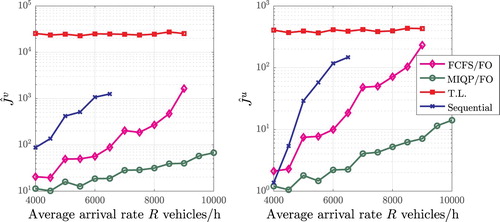
Figure 4. Energy cost of coordination: percentage increase ${\hat{E}}^{\mathrm{\%}}$ (solid line, right axis); and CoC increase ${\hat{E}}^{\mathrm{CoC}}$ (pale lines, left axis). Colour coding as in Figure 3.

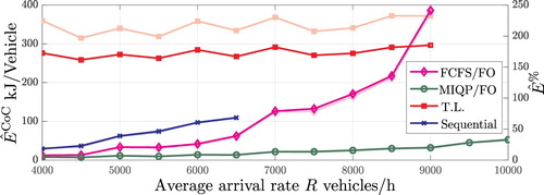
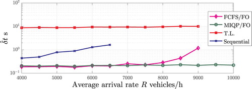
Figure 5. Travel time delay compared to the Overpass solution.

Traffic light vs. automated controllers: The difference is rather large for average arrival rates low enough to not cause congestion. For low arrival rates, all automated controllers give small increases in energy consumption compared to the overpass solution, induce a small travel time delay and are orders of magnitude better than the Traffic Light in terms of the quadratic objective. We highlight in particular the performance of the proposed MIQP/FO controller in terms of energy consumption: it can handle very high traffic intensities ($R=\mathrm{10,000}$) with an energy increase not exceeding 40% of the Overpass controller energy. This is mainly due to the automated controllers' ability to coordinate the vehicles without forcing them to stop.

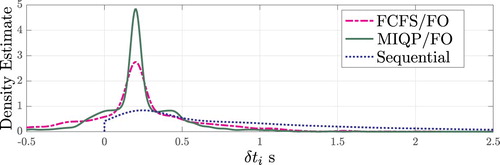
Effect of joint optimisation: The performance of the different automated controllers increases with added complexity. FCFS/FO outperforms the sequential controller in all performance metrics. Additionally, MIQP/FO outperforms FCFS/FO in all performance metrics except the travel-time delay, where the FCFS/FO and MIQP/FO perform closely for $R\le 8000$ vehicles/h, with close to zero average delay. This is a consequence of the joint optimisation of the trajectories, which increases the velocity of some vehicles (resulting in ‘negative’ delays), and decreases velocities of other vehicles (resulting in positive delays), with an average close to zero. This is further illustrated in Figure 6, which shows estimates of the distribution of travel time delays under the three automated controllers.

Figure 6. Estimate of the distribution of the observed $\delta t_i$ for R = 6000 vehicles/h.

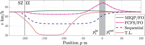
A closer look at the vehicle velocities: The results in Figures 4 and 5 are explained by the velocity profiles in Figure 7. In particular, smaller velocity variations (decelerations) lead to more efficient coordination policies. The maximum and minimum velocity profiles of the MIQP/FO are smoother than the ones of the FCFS/FO scheme (see e.g. around the 5-minute mark). A closer look at one spike is provided in Figure 8, which shows the position-velocity profiles from the same vehicle for the different controllers. As the figure illustrates, the spikes occur when the optimal solution to the fixed, FCFS-crossing order problem strongly accelerates some vehicles through the intersection. While such manoeuvre is costly, it allows other vehicles to use the intersection more efficiently. Even though a slight velocity increase also results from the MIQP/FO controller, the magnitude is significantly lower and is performed well before the intersection starts. This reveals the MIQP's ability to select crossing orders that are convenient for the underlying fixed-order coordination problem.

Figure 7. Average velocity (coloured lines) and velocity intervals (grey surface) in a scenario with R = 6000 vehicles/hour.

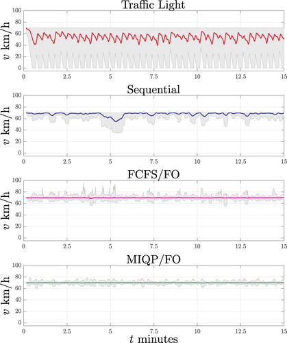
Figure 8. Position-velocity trajectories of one vehicle from the scenario with R = 6000 vehicles/hour. The grey bar corresponds to positions inside the intersection, 0 being the centre, whereas the grey line demarcates the beginning of the IZ.

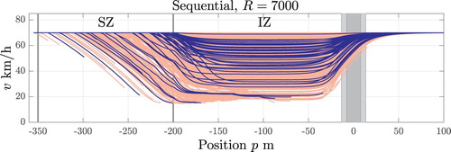
4.3. Failure of the FCFS/FO and Sequential Controllers

In the simulation with R = 7000 vehicles per hour, the Sequential controller caused some vehicles inside the IZ to reduce their velocity significantly. In turn, this caused vehicles outside the IZ to slow down in order to avoid collisions and satisfy Assumption 2.3. Eventually, a significant velocity decrease propagated to the beginning of the SZ, such that the scenario was considered congested and the simulation stopped. For the FCFS/FO controller, the simulation was stopped after it performed worse than the Traffic Light (c.f. Figure 4).

4.3.1. Causes of the FCFS/FO failure

We first note that the fixed-order problem is expected to assign a relatively higher control effort and result in larger velocity deviations for Cars than Trucks due to the objective weighting (cf. objective (15(15) $J_i(x_i,u_i)=m_i(Q_i^{\mathrm{f}}(v_{i,K}-v^r{)}^2+\sum _{k=0}^K{Q}_i(v_{i,k}-v^r{)}^2+R_i{u}_{i,k}^2),$(15) ) and Table 2). Regardless of how the crossing order is selected, the vehicles of the Car type are therefore expected to perform more aggressive manoeuvres in general, and attaining the maximum and minimum velocities (cf. the velocity intervals of Figure 7).

However, the magnitude of both control effort and velocity deviations depend on the selected crossing order: a Car which crosses after a Truck under the FCFS policy could be commanded to slow down significantly to decrease the total cost, whereas an alternative order inducing the Car to cross before the Truck would result in a velocity increase. When the traffic load increases, such accelerations occur farther from the intersection with lower minimum values, and the lower velocities are kept for longer periods of time.

This effect is illustrated in Figure 9, which presents the velocity as a function of distance for all vehicles resulting from the FCFS/FO controller for average arrival rates R = 8000, R = 8500 and R = 9000 vehicles/h, and from the MIQP/FO controller for R = 9000. As the figure shows, for increasing R, the FCFS/FO controller indeed results in harsher accelerations and both lower minimum velocities at greater distances from the intersection and longer periods of low velocities. Note in particular the almost triangular velocity profiles of many Cars as the intersection is crossed, which corresponds to periods of (constant) maximum acceleration and deceleration. This behaviour is primarily seen in Cars: the optimal solution is often to first slow down to favour Trucks (due to the weighting of their objectives with $m_i$) and thereafter to cross the intersection as fast as possible to not block access for others. Moreover, we note that the velocity decreases closer to the SZ start with increasing R since safety must be enforced and the FCFS/FO is brought closer to causing congestion.

Figure 9. Speed profiles of Trucks (dark) and Cars (pale). The solid bars and the two vertical lines mark the intersection for Cars (dark) and Trucks (light) and the start of the SZ and IZ, respectively.

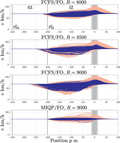
Finally, we note that while both the FCFS/FO and MIQP/FO controllers actuate Cars more than Trucks, the effect is much more pronounced in the former. In particular, the two bottom plots in Figure 9 illustrate the difference for the same generation pattern and show that both vehicle types are actuated less under the MIQP/FO controller. This results in smoother trajectories and almost no velocity reduction outside the IZ, thus demonstrating the benefit of selecting a crossing order which takes the objective function and constraints into account at least approximately.

4.3.2. Causes of the sequential controller failure

In the sequential controller case, no vehicle increases its velocity to favour another, and collisions are avoided solely through velocity reductions. This propagates backwards on each lane and can even be amplified depending on the distance between the vehicles involved. The velocity profiles from the congested R = 7000 vehicles/h scenario with the Sequential controller are shown in Figure 10, where significant velocity reductions are present in the entire IZ, and propagate further backwards until they reach $p_{SZ}^{\mathrm{e}}$ and the simulation is terminated.

Figure 10. Velocity profiles for vehicles in the scenario with R = 7000, where the sequential controller failed. Colouring as in Figure 9.

5. Conclusion

In this paper, we introduced a closed-loop controller for coordination of automated vehicles at intersections, based on a simultaneous yet approximate solution of an optimal control problem. We presented simulation results where the controller was compared against two simpler approaches for automated coordination, a traffic light coordination mechanism and a physical separation of the roads. The results demonstrate that all automated controllers outperform the traffic light system under low to medium traffic intensities and that significant gains are achieved with increasing controller complexity. In particular, we showed that by jointly optimising both the crossing order and the vehicle trajectories, large improvements are obtained compared to all other considered methods, both in terms of performance and capacity. This serves as a motivation for considering the more sophisticated controllers.

We also emphasise that even though the proposed MIQP/FO controller relies on approximations and is sub-optimal, the cost increase stemming from coordination is remarkably small, even for high traffic intensities. At the same time, the improvement over both traffic lights and the simpler coordination mechanisms is large, in particular for higher traffic intensities. The improvement is obtained at the price of a higher computational demand, which, however, can be maintained within reasonable limits by a tailored distributed problem formulation [38] for the continuous part of the problem. The solution times of the MIQP have also been observed to be real-time feasible, especially when the amount of coordinated vehicles is less than 30. However, integer feasible solutions with a small optimality gap were typically quickly computed for larger scenarios. It would, therefore, be possible to stop the MIQP solver prematurely while retaining persistent safety, at the expense of possible sub-optimality. A deeper investigation of such aspects will be the subject of future research.

Finally, it is worth recalling that the results provided in this paper formally hold in the nominal case only. That is, the results on persistent safety in Section 2.5 may not hold in the presence of model uncertainties, external disturbances and measurement noise. Nevertheless, experimental results have demonstrated the resilience of the proposed closed-loop coordination algorithms. Additionally, the algorithm can be adapted to explicitly account for uncertainty and, therefore, provide robustness guarantees.

Disclosure statement

No potential conflict of interest was reported by the author(s).

ORCID

Robert Hult  http://orcid.org/0000-0002-1337-3880

Notes

1 In case $v_i(t_{i,r}^{\mathrm{in}})=0$, $t_{i,r}^{\mathrm{in}}$ is not uniquely defined by $p_i(t_{i,r}^{\mathrm{in}})=p_{r,i}^{\mathrm{in}}$, but rather by definition $t_{r,i}^{\mathrm{in}}=mint\mathrm{s}.\mathrm{t}.p_i(t_{i,r}^{\mathrm{in}})=p_{r,i}^{\mathrm{in}}$. Alternatively, one can modify (1(1a) $\begin{array}{rl}{\dot{x}}_i(t)& =f_i(x_i(t),u_i(t)),\end{array}$(1a) ) so that $\dot{p}\ge ϵ$, for some small $ϵ>0$. Since $v_i(t_{i,r}^{\mathrm{in}})=0$ will be rarely encountered in practice, we assume $v_i(t_{i,r}^{\mathrm{in}})\ne 0$ for ease of presentation.

References

- Sjöberg K, Andres P, Buburuzan T, et al. Cooperative intelligent transport systems in Europe: current deployment status and outlook. IEEE Veh Technol Mag. 2017;12(2):89–97. doi: 10.1109/MVT.2017.2670018
- Chen S, Hu J, Shi Y, et al. Vehicle-to-everything (V2X) services supported by LTE-based systems and 5G. IEEE Commun Standards Mag. 2017;1(2):70–76. doi: 10.1109/MCOMSTD.2017.1700015
- Simon M, Hermitte T, Page Y. Intersection road accident causation: a European view. In: International Technical Conference on the Enhanced Safety of Vehicles; Stuttgart, Germany; 2009. p. 1–10.
- Li M, Boriboonsomsin K, Wu G, et al. Traffic energy and emission reductions at signalized intersections: a study of the benefits of advanced driver information. Int J Intell Transp Syst Res. 2009;7(1):49–58.
- Colombo A, Del Vecchio D. Efficient algorithms for collision avoidance at intersections. In: ACM International Conference on Hybrid Systems: Computation and Control; 2012; Beijing, China. p. 145–154.
- Wymeersch H, de Campos GR, Falcone P, et al. Challenges for cooperative its: Improving road safety through the integration of wireless communications, control, and positioning. In: 2015 International Conference on Computing, Networking and Communications (ICNC); Feb; 2015; Anaheim, CA, USA. p. 573–578.
- Chen L, Englund C. Cooperative intersection management: a survey. IEEE Trans Intell Transp Syst. 2016;17(2):570–586. doi: 10.1109/TITS.2015.2471812
- Rios-Torres J, Malikopoulos AA. A survey on the coordination of connected and automated vehicles at intersections and merging at highway on-ramps. IEEE Trans Intell Transp Syst. 2017;18:1066–1077. doi: 10.1109/TITS.2016.2600504
- Dresner K, Stone P. A multiagent approach to autonomous intersection management. J Artif Intell Res. 2008;31(1):591–656. doi: 10.1613/jair.2502
- Milanes V, Perez J, Onieva E, et al. Controller for urban intersections based on wireless communications and fuzzy logic. IEEE Trans Intell Transp Syst. 2010;11(1):243–248. doi: 10.1109/TITS.2009.2036595
- Kowshik H, Caveney D, Kumar PR. Provable systemwide safety in intelligent intersections. IEEE Trans Veh Technol. 2011;60(3):804–818. doi: 10.1109/TVT.2011.2107584
- de Campos GR, Falcone P, Sjöberg J. Autonomous cooperative driving: a velocity-based negotiation approach for intersection crossing. In: 16th International IEEE Conference on Intelligent Transportation Systems; Oct; 2013; The Hague, Netherlands. p. 1456–1461.
- de Campos GR, Falcone P, Wymeersch H, et al. Cooperative receding horizon conflict resolution at traffic intersections. In: 53rd IEEE Conference on Decision and Control; Dec; 2014; Los Angeles, CA, USA. p. 2932–2937.
- Qian X, Grégoire J, de La Fortelle A, et al. Decentralized model predictive control for smooth coordination of automated vehicles at intersection. In: European Control Conference; July; 2015; Linz, Austria. p. 3452–3458.
- Kim K, Kumar PR. An mpc-based approach to provable system-wide safety and liveness of autonomous ground traffic. IEEE Trans Autom Control. 2014;59(12):3341–3356. doi: 10.1109/TAC.2014.2351911
- Molinari F, Raisch J. Automation of road intersections using consensus-based auction algorithms. In: 2018 Annual American Control Conference (ACC); June; 2018; Milwaukee, WI, USA. p. 5994–6001.
- Makarem L, Gillet D. Model predictive coordination of autonomous vehicles crossing intersections. In: 16th International IEEE Conference on Intelligent Transportation Systems; Oct; 2013; The Hague, Netherlands. p. 1799–1804.
- Katriniok A, Kleibaum P, Josevski M. Distributed model predictive control for intersection automation using a parallelized optimization approach. IFAC-PapersOnLine. 2017;50(1):5940–5946. doi: 10.1016/j.ifacol.2017.08.1492
- Sprodowski T, Pannek J. Stability of distributed MPC in an intersection scenario. J Phys Conf Ser. 2015;659:012049. doi: 10.1088/1742-6596/659/1/012049
- Britzelmeier A, Gerdts M. Non-linear model predictive control of connected, automatic cars in a road network using optimal control methods. IFAC-PapersOnLine. 2018;51(2):168–173. doi: 10.1016/j.ifacol.2018.03.029
- Malikopoulos AA, Cassandras CG, Zhang YJ. A decentralized energy-optimal control framework for connected automated vehicles at signal-free intersections. Automatica. 2018;93:244–256. doi: 10.1016/j.automatica.2018.03.056
- Zhang Y, Cassandras CG. Decentralized optimal control of connected automated vehicles at signal-free intersections including comfort-constrained turns and safety guarantees. Automatica. 2019;109:108563. doi: 10.1016/j.automatica.2019.108563
- Katriniok A, Sopasakis P, Schuurmans M, et al. Nonlinear model predictive control for distributed motion planning in road intersections using PANOC. In: IEEE Conference on Decision and Control; Vol. 12; Nice, France; 2019.
- Murgovski N, de Campos GR, Sjöberg J. Convex modeling of conflict resolution at traffic intersections. In: IEEE Conference on Decision and Control; Dec; 2015; Osaka, Japan. p. 4708–4713.
- Riegger L, Carlander M, Lidander N, et al. Centralized mpc for autonomous intersection crossing. In: IEEE International Conference on Intelligent Transportation Systems; Nov; 2016; Rio de Janeiro, Brazil. p. 1372–1377.
- Tallapragada P, Cortés J. Coordinated intersection traffic management. IFAC-PapersOnLine. 2015;48(22):233–239. doi: 10.1016/j.ifacol.2015.10.336
- Hult R, Zanon M, Gros S, et al. Primal decomposition of the optimal coordination of vehicles at traffic intersections. In: IEEE 55th Conference on Decision and Control; Dec; 2016; Las Vegas, NV, USA. p. 2567–2573.
- Zanon M, Gros S, Wymeersch H, et al. An asynchronous algorithm for optimal vehicle coordination at traffic intersections. 20th IFAC World Congress; Toulouse, France; 2017.
- Jiang Y, Zanon M, Hult R, et al. Distributed algorithm for optimal vehicle coordination at traffic intersections. IFAC-PapersOnLine. 2017;50(1):11577–11582. doi: 10.1016/j.ifacol.2017.08.1511
- Shi J, Zheng Y, Jiang Y, et al. Distributed control algorithm for vehicle coordination at traffic intersections. In: European Control Conference; June; 2018; Limasol, Cyprus. p. 1166–1171.
- Kneissl M, Molin A, Esen H, et al. A feasible mpc-based negotiation algorithm for automated intersection crossing. In: European Control Conference; 06; 2018; Limasol, Cyprus. p. 1282–1288.
- Kamal MAS, Imura J, Hayakawa T, et al. A vehicle-intersection coordination scheme for smooth flows of traffic without using traffic lights. IEEE Trans Intell Transp Syst. 2015;16(3):1136–1147. doi: 10.1109/TITS.2014.2354380
- Li B, Zhang Y, Zhang Y, et al. Near-optimal online motion planning of connected and automated vehicles at a signal-free and lane-free intersection. In: IEEE Intelligent Vehicle Symposium; 06; 2018; Changshu, China. p. 1432–1437.
- Bali C, Richards A. Merging vehicles at junctions using mixed-integer model predictive control. In: European Control Conference; 06; 2018; Limasol, Cyprus. p. 1740–1745.
- Hult R, Campos GR, Falcone P, et al. An approximate solution to the optimal coordination problem for autonomous vehicles at intersections. In: 2015 American Control Conference (ACC); July; 2015; Chicago, IL, USA. p. 763–768.
- Hult R, Zanon M, Gros S, et al. Energy-optimal coordination of autonomous vehicles at intersections. In: European Control Conference; June; 2018; Limasol, Cyprus. p. 602–607.
- Hult R, Zanon M, Gros S, et al. An miqp-based heuristic for optimal coordination of vehicles at intersections. In: IEEE Conference on Decision and Control; Dec; 2018; Miami Beach, FL, USA. p. 2783–2790.
- Hult R, Zanon M, Gros S, et al. Optimal coordination of automated vehicles at intersections: theory and experiments. IEEE Trans Control Syst Technol. 2018;27(6):2510–2525. doi: 10.1109/TCST.2018.2871397
- Hult R, Zanon M, Gros S, et al. Optimal coordination of automated vehicles at intersections with turns. In: European Control Conference; Naples, Italy; 2019.
- Dresner K, Stone P. Multiagent traffic management: a reservation-based intersection control mechanism. In: Proceedings of the Third International Joint Conference on Autonomous Agents and Multiagent Systems; July; 2004; New York, NY, USA. p. 530–537.
- Lee J, Park B. Development and evaluation of a cooperative vehicle intersection control algorithm under the connected vehicles environment. IEEE Trans Intell Transp Syst. 2012;13(1):81–90. doi: 10.1109/TITS.2011.2178836
- Rawlings J, Mayne D. Model predictive control: theory and design. Madison (WI): Nob Hill; 2009.
- Bock H, Plitt K. A multiple shooting algorithm for direct solution of optimal control problems. IFAC Proc Volumes. 1984;17(2):1603–1608. 9th IFAC World Congress. doi: 10.1016/S1474-6670(17)61205-9
- Hult SR, Zanon M, Gros S, et al. Animated illustration of the MIQP/FO controller [Internet]; 2019. [cited 2019 Feb 26]. Available from: https://youtu.be/hUWQoaiqdAY.
- Hult R, Zanon M, Gros S, et al. Optimal coordination of three cars approaching an intersection [Internet]. 2017. [cited 2019 Feb 26]. Available from: https://youtu.be/nYSXvnaNRK4.
- Murgovski N, Johannesson LM, Egardt B. Optimal battery dimensioning and control of a CVT PHEV powertrain. IEEE Trans Veh Technol. 2014;63(5):2151–2161. doi: 10.1109/TVT.2013.2290601