Unsteady-state brush theory

Abstract

This paper deals with unsteady-state brush tyre models. Starting from tyre-road contact theory, we provide a full analytical solution to the partial differential equations (PDEs) describing the bristle deformation in the adhesion region of the contact patch. We show that the latter can be divided in two different regions, corresponding to two different domains for the solution of the governing PDEs of the system. In the case of constant sliding speed inputs, the steady-state solution coincides with the one provided by the classic steady-state brush theory. For a rectangular contact patch and parabolic pressure distribution, the time trend of the shear stresses is investigated. For the pure interactions (longitudinal, lateral and camber), some important conclusions are drawn about the relaxation length. Finally, an approach to derive simplified formulae for the tangential forces arising in the contact patch is introduced; the tyre formulae obtained by using the proposed approach are not based on the common slip definition, and can be employed when the rolling speed approaches zero. The outlined procedure is applied to the cases of linear tyre forces and parabolic pressure distribution.

Keywords:

• Tyre dynamics
• tyre model
• brush model
• transport equation
• nonlinear dynamics

View correction statement:

Correction

1. Introduction

In the last decades, a great deal of research has been dedicated to the development of model-based control strategies to be employed in emergency braking and handling dynamic scenarios [1]. Two main factors influencing the braking capacity of a vehicle are tyre-road friction and available braking torque. Both are difficult to determine precisely due to modelling complexities and variations in the operating conditions. On the other hand, a properly descriptions of the tyre-road contact mechanisms is also crucial to improve energy efficiency [2].

In literature different tyre models have been proposed over the recent years. Some very advanced FEM or Multibody models [3–5] are capable of capturing many phenomena related to the tyre dynamics. Nevertheless, their intrinsic complexity makes them computationally demanding, and eventually unsuitable for real-time applications. As a consequence, they are mainly adopted to evaluate static properties of tyres, including stiffness, resonant frequencies and vibration modes.

In order to fulfill the real-time requirement, several simpler approaches for tyre modelling have been developed. Nowadays, one of the most widespread technique is Pacejka's ‘Magic Formula’ (MF) [6], describing tyre steady-state tyre characteristics by means of a wide set of different fitting parameters. However, due to its pure empirical nature, the model is non-intuitive with respect to physical interpretations.

In contrast, the so-called brush models [7–9] are grounded on few physical assumptions. They require only a small number of coefficients to be parametrised and are able to provide a qualitatively accurate description of the forces exchanged between the tyre and the road. Their main drawback is usually connected to a possible mismatch to the experimental data due to the simplified modelling approach.

To overcome this disadvantage, some efforts have been directed towards a more detailed description of the contact patch. For example, in [10], the effect of different pressure distributions – including asymmetrical ones and higher-order polynomial – on the tyre forces has been investigated extensively. Also, a three-dimensional brush model for describing longitudinal characteristics of the tyre in steady-state conditions has been presented in [11]. In [12], the author has successfully extended Kalker's theory to rubber tyres starting from a semi-analytical model normally employed in studies related to the wheel-rail contact mechanics. In [13], the effect of the thermal and frictional effects on ground vehicle performance has been studied by employing a simplified model for tire wear estimation. Finally, other works [14–16] have been substantially aimed at estimating the road friction coefficient from forces and slip measurements by assuming the tyre behaviour following some enhanced brush models.

Like Pacejka's MF, steady-state brush models provide an analytical representation of the tyre forces as a function of the slip variable, a mathematical quantity which cannot be defined at zero rolling speed. This makes slip-based tyre formulae inappropriate to model close-to-standstill or wheel-locked scenarios. This is the main reason why several attempts have been made in order to include dynamic properties capable of handling transient phases.

A very early attempt to address the issue dates from the late 80s. In the context of railway dynamics, Kalker pioneered an analytical solution for the case of pure longitudinal slip in [17]. The proposed solution was also proved to be consistent with the main underlying assumptions of the model, but its derivation was omitted completely. More advanced investigations were also carried out by employing specially developed tools [18] or numerical methods [19].

Amongst the transient models for road vehicle dynamics, the best known are perhaps the Single Point Contact Model developed by Pacejka [6], the ‘LuGre’ model [1], and the full-transient one presented by Guiggiani in [7] and more recently in [8]. The first model, introduced in [6], renounces to deal with the bristle dynamics, and can be seen as an enhanced steady-state brush model which takes into account the deformation of the tyre carcass. This allows to provide a transient solution for both the lateral force and the self-aligning moment resulting from a first order differential equation almost without introducing any computational drawback. In the ‘Lugre’ formulation [1], an internal friction parameter is used to represent the shear stresses exerted at the tyre-road interface and the friction-induced hysteresis. Some specially developed functions are also included in order to fit Pacejka's curves. Finally, the latter takes into account both the bristle and the carcass dynamics, leading to a more complete formulation. In [7,8], the response to pure lateral and longitudinal slip input is investigated separately and the author proposes an iterative method to compute the position of the breakaway point and the resulting force and moments generated within the contact patch. Lastly, other authors have proposed solutions based on finite difference approximations [20], or on interconnected bristle models [21]. The TreadSim package implemented by Pacejka [6] is also based on the discretisation of the contact patch. It is a detailed description of the tyre tread which allows to account for several features – conicity, flexible carcass – and operative conditions – sliding-dependent friction coefficient, combined slips, irregular pressure distributions – which would otherwise make the analytical approach completely inadequate.

From the excursus above, it is glaring that an extremely simple model capable of exhaustively describing tyre characteristics during transients has not been developed yet. Indeed, whilst the enhanced MF versions can macroscopically reflect unsteady-state tyre behaviours, a detailed understanding of the microscopic phenomena occurring in the contact patch is still lacking. Conversely, more exhaustive formulations require numerical techniques and don't come with a close form solution.

Hence, in this paper, a novel theory of unsteady-state brush models inspired by Kalker's studies [17] is presented. The closed-form solution for the deformation of the tyre carcass and the bristles representing the tread is derived by using the method of characteristics. It is also shown that it can be determined uniquely depending on the boundary or initial condition. The analysis is extended to a very general case – which includes longitudinal, lateral and rotational slips – and allows for some fundamental considerations about the time-varying trend of the shear stresses arising inside the contact patch.

The analysis is further deepened when the compliance of the tyre carcass is neglected. This allows for some simplification and makes the problem suitable to cope with from a pure theoretical perspective. Some interesting results are drawn which relate with the simultaneous existence of different sticking and sliding regions inside the contact patch during the transient of the bristles.

Then, a simplified approach to derive a family of transient tyre formulae generalising the already-existing ones, called ‘two-regime formulae’, is discussed. This new class of model accounts for both the transient of the bristles and the compliance of the tyre carcass, being of more practical interest. The resulting expressions for the tangential forces acting at the tyre-road interface are not based on the slip quantity, and can be successfully employed to describe some phenomena that are not normally predicted by the classic steady-state brush models.

This paper is organised as follows: in Section 2, the derivation of the tyre-road contact equations is given and all the main assumptions are outlined. The general solution for the tyre-road contact equations in the adhesion region is derived in Section 3 and some comparison with numerical solutions are shown. In Section 4, under the assumptions of rectangular contact patch and parabolic pressure distribution, the analysis is extended further for the case of pure interactions (longitudinal, lateral and camber) and an estimation of the relaxation length is provided. A simplified approach to derive a more straightforward expression for the transient tyre formulae is first illustrated in Section 5 in general terms, then an example is also presented in the case of linear tyre forces. Finally, conclusions and further developments are drawn in Section 6.

2. Governing equations of the brush tyre model

2.1. Tyre-road contact equations

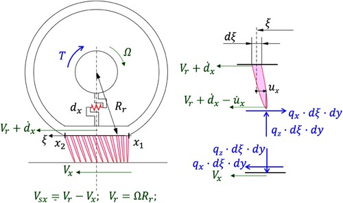
Apart from the different nomenclature and some minor considerations about the constitutive relation and related boundary conditions, the formulation of the brush model in this section is entirely based on the one proposed by Guiggiani in [7,8]. The tyre-road contact equations are derived by using the Eulerian approach. Let us consider a finite control area $\mathcal{S}(x,y,0)=\left\{\right(x,y,z)\in {\mathbb{R}}^3:x_T(y)\le x\le x_L(y),y_L\le y\le y_R,z=0\}$ in the absolute reference frame $({\hat{\mathit{e}}}_x,{\hat{\mathit{e}}}_y,{\hat{\mathit{e}}}_z)$, where $l(y,{\mathit{\rho }}_l(t\left)\right)=x_L(y,{\mathit{\rho }}_{x_L}(t\left)\right)-x_T(y,{\mathit{\rho }}_{x_T}(t\left)\right)$ and $w(y,{\mathit{\rho }}_w(t\left)\right)=y_R\left({\mathit{\rho }}_{y_R}\right(t\left)\right)-y_L\left({\mathit{\rho }}_{y_L}\right(t\left)\right)$ are the length of the contact patch at the coordinate y and the maximum tyre width, respectively. The functions $\mathit{\rho }$ parametrise the shape of the contact patch and may depend on different variables, such as the vertical force acting on the tyre. The vertical dimension is also assumed to be zero since the carcass and the tread only undergo deformations in the longitudinal and lateral directions. We start by introducing the tyre-road contact equations in vectorial form as follows [7,8,22] (1a) $\begin{array}{rl}{\mathit{v}}_s(\mathit{x},t)& =\mathbf{0}⟺\Vert {\mathit{q}}_t(\mathit{x},t)\Vert <{\mu }_s{q}_z(\mathit{x},t),\end{array}$(1a) (1b) $\begin{array}{rl}{\mathit{q}}_t(\mathit{x},t)& =-{\mu }_d{q}_z(\mathit{x},t)\frac{{\mathit{v}}_s(\mathit{x},t)}{\Vert {\mathit{v}}_s(\mathit{x},t)\Vert }⟺{\mathit{v}}_s(\mathit{x},t)\ne \mathbf{0},\end{array}$(1b) in which ${\mathit{v}}_s(\mathit{x},t)=\left[v_{sx}\right(\mathit{x},t\left)v_{sy}\right(\mathit{x},t){]}^T$ is the micro-sliding velocity of a bristle at position $\mathit{x}$ and time t, ${\mathit{q}}_t(\mathit{x},t)=\left[q_x\right(\mathit{x},t\left)q_y\right(\mathit{x},t){]}^T$ is the tangential force per unit of area applied on that bristle, $q_z(\mathit{x},t)$ is the vertical pressure acting in the contact patch and ${\mu }_s$ and ${\mu }_d$ are the static and dynamic friction coefficients, respectively. We point out that (1(1a) $\begin{array}{rl}{\mathit{v}}_s(\mathit{x},t)& =\mathbf{0}⟺\Vert {\mathit{q}}_t(\mathit{x},t)\Vert <{\mu }_s{q}_z(\mathit{x},t),\end{array}$(1a) ) are only valid under a memoryless friction assumption.

The relative micro-sliding velocity of the tread bristle at position $\mathit{x}$ contacting the road reads (2) ${\mathit{v}}_s(\mathit{x},t)={\mathit{V}}_s\left(t\right)+{\mathit{\omega }}_z\left(t\right)\times (\mathit{x}+{\mathit{u}}_t(\mathit{x},t\left)\right)+\frac{\mathrm{d}{\mathit{u}}_t(\mathit{x},t)}{\mathrm{d}t}+\dot{\mathit{d}}\left(t\right).$(2) In (2(2) ${\mathit{v}}_s(\mathit{x},t)={\mathit{V}}_s\left(t\right)+{\mathit{\omega }}_z\left(t\right)\times (\mathit{x}+{\mathit{u}}_t(\mathit{x},t\left)\right)+\frac{\mathrm{d}{\mathit{u}}_t(\mathit{x},t)}{\mathrm{d}t}+\dot{\mathit{d}}\left(t\right).$(2) ), ${\mathit{V}}_s\left(t\right)$ is the macro-sliding velocity, defined as the difference between the speed of the rigid equivalent tyre and that of the road. ${\mathit{\omega }}_z\left(t\right)={\mathit{\omega }}_{1z}\left(t\right)-{\mathit{\omega }}_{2z}\left(t\right)$ is the spin angular speed, with ${\mathit{\omega }}_{1z}\left(t\right)=-\mathrm{\Omega }\left(t\right)\sin \gamma \left(t\right){\hat{\mathit{e}}}_z$ the normal component of the rolling speed due to camber and ${\mathit{\omega }}_{2z}\left(t\right)=-\dot{\psi }\left(t\right){\hat{\mathit{e}}}_z$ the steering speed.¹ Finally, ${\mathit{u}}_t(\mathit{x},t)$ and $\mathit{d}\left(t\right)$ are the tangential deformations of the bristle and carcass, respectively. The latter is also modelled as a single point body (see Figure 1).

Figure 1. Tyre schematic for the pure longitudinal problem ($V_y\left(t\right)={\omega }_z\left(t\right)=0$). The bristles and the tyre carcass (modelled as a linear spring) are drawn in red. The generalised forces acting on the tyre-wheel system are represented in blue. The speeds are finally given in green. The dot notation stands for total derivative with respect to time. The local variable $\xi =x_L(y,{\mathit{\rho }}_{x_L}(t\left)\right)-x$ is referred as the distance from the leading edge.

Introducing the gradient operator ∇, Equation (2(2) ${\mathit{v}}_s(\mathit{x},t)={\mathit{V}}_s\left(t\right)+{\mathit{\omega }}_z\left(t\right)\times (\mathit{x}+{\mathit{u}}_t(\mathit{x},t\left)\right)+\frac{\mathrm{d}{\mathit{u}}_t(\mathit{x},t)}{\mathrm{d}t}+\dot{\mathit{d}}\left(t\right).$(2) ) can be recast as (3) ${\mathit{v}}_s(\mathit{x},t)={\mathit{V}}_s\left(t\right)+{\mathit{\omega }}_z\left(t\right)\times (\mathit{x}+{\mathit{u}}_t(\mathit{x},t\left)\right)+\frac{\mathrm{\partial }{\mathit{u}}_t(\mathit{x},t)}{\mathrm{\partial }t}+\dot{\mathit{x}}\cdot \mathrm{\nabla }{\mathit{u}}_t(\mathit{x},t)+\dot{\mathit{d}}\left(t\right),$(3) where the quantity $\dot{\mathit{x}}$ is approximatively (4) $\dot{\mathit{x}}\simeq -\mathrm{\Omega }\left(t\right)R_r\left(t\right){\hat{\mathit{e}}}_x:=-V_r\left(t\right){\hat{\mathit{e}}}_x,$(4) with $R_r\left(t\right)$ the so-called effective rolling radius and $V_r\left(t\right)$ the rolling speed.

Specifying the other quantities in (3(3) ${\mathit{v}}_s(\mathit{x},t)={\mathit{V}}_s\left(t\right)+{\mathit{\omega }}_z\left(t\right)\times (\mathit{x}+{\mathit{u}}_t(\mathit{x},t\left)\right)+\frac{\mathrm{\partial }{\mathit{u}}_t(\mathit{x},t)}{\mathrm{\partial }t}+\dot{\mathit{x}}\cdot \mathrm{\nabla }{\mathit{u}}_t(\mathit{x},t)+\dot{\mathit{d}}\left(t\right),$(3) ) and neglecting the higher order terms, the new tyre-road contact equations in scalar form [23,24] read (5a) $\begin{array}{rl}{v}_{sx}(\mathit{x},t)& =V_{sx}\left(t\right)-{\omega }_z\left(t\right)y+\frac{\mathrm{\partial }{u}_x(\mathit{x},t)}{\mathrm{\partial }t}-V_r\left(t\right)\frac{\mathrm{\partial }{u}_x(\mathit{x},t)}{\mathrm{\partial }x}+{\dot{d}}_x\left(t\right),\end{array}$(5a) (5b) $\begin{array}{rl}{v}_{sy}(\mathit{x},t)& =V_{sy}\left(t\right)+{\omega }_z\left(t\right)x+\frac{\mathrm{\partial }{u}_y(\mathit{x},t)}{\mathrm{\partial }t}-V_r\left(t\right)\frac{\mathrm{\partial }{u}_y(\mathit{x},t)}{\mathrm{\partial }x}+{\dot{d}}_y\left(t\right).\end{array}$(5b) Performing the coordinate change (6) $\mathit{\xi }=\left[\begin{array}{c}\xi \\ \eta \\ \zeta \end{array}\right]=\left[\begin{array}{c}{x}_L\left(y\right)-x\\ y\\ z\end{array}\right].$(6) Equation (5(5a) $\begin{array}{rl}{v}_{sx}(\mathit{x},t)& =V_{sx}\left(t\right)-{\omega }_z\left(t\right)y+\frac{\mathrm{\partial }{u}_x(\mathit{x},t)}{\mathrm{\partial }t}-V_r\left(t\right)\frac{\mathrm{\partial }{u}_x(\mathit{x},t)}{\mathrm{\partial }x}+{\dot{d}}_x\left(t\right),\end{array}$(5a) ) finally becomes (7a) $\begin{array}{rl}{v}_{sx}(\mathit{\xi },t)& =V_{sx}\left(t\right)-{\omega }_z\left(t\right)\eta +\frac{\mathrm{\partial }{u}_x(\mathit{\xi },t)}{\mathrm{\partial }t}+V_r\left(t\right)\frac{\mathrm{\partial }{u}_x(\mathit{\xi },t)}{\mathrm{\partial }\xi }+{\dot{d}}_x\left(t\right),\end{array}$(7a) (7b) $\begin{array}{rl}{v}_{sy}(\mathit{\xi },t)& =V_{sy}\left(t\right)+{\omega }_z\left(t\right)\left[x_L\right(\eta )-\xi ]+\frac{\mathrm{\partial }{u}_y(\mathit{\xi },t)}{\mathrm{\partial }t}+V_r\left(t\right)\frac{\mathrm{\partial }{u}_y(\mathit{\xi },t)}{\mathrm{\partial }\xi }+{\dot{d}}_y\left(t\right).\end{array}$(7b) Equations (7(7a) $\begin{array}{rl}{v}_{sx}(\mathit{\xi },t)& =V_{sx}\left(t\right)-{\omega }_z\left(t\right)\eta +\frac{\mathrm{\partial }{u}_x(\mathit{\xi },t)}{\mathrm{\partial }t}+V_r\left(t\right)\frac{\mathrm{\partial }{u}_x(\mathit{\xi },t)}{\mathrm{\partial }\xi }+{\dot{d}}_x\left(t\right),\end{array}$(7a) ) are two inhomogeneous linear partial differential equations (more specifically, transport equations), with initial and boundary conditions given by (8a) $\begin{array}{rl}{\mathit{u}}_t\left(\xi \right(\eta ),\eta ,0)& ={\mathit{u}}_t^0\left(\mathit{\xi }\right),\end{array}$(8a) (8b) $\begin{array}{rl}{\mathit{q}}_t(0,\eta ,t)& =\mathbf{0}.\end{array}$(8b) The first of (8(8a) $\begin{array}{rl}{\mathit{u}}_t\left(\xi \right(\eta ),\eta ,0)& ={\mathit{u}}_t^0\left(\mathit{\xi }\right),\end{array}$(8a) ) imposes the initial condition for the deformation of the bristle at the time t = 0. The latter prescribes that the tangential force at the entrance of the contact patch must be zero. This follows from the hypothesis of continuous traction distribution at the leading edge $\xi \left(\eta \right)$ [25]. To solve (7(7a) $\begin{array}{rl}{v}_{sx}(\mathit{\xi },t)& =V_{sx}\left(t\right)-{\omega }_z\left(t\right)\eta +\frac{\mathrm{\partial }{u}_x(\mathit{\xi },t)}{\mathrm{\partial }t}+V_r\left(t\right)\frac{\mathrm{\partial }{u}_x(\mathit{\xi },t)}{\mathrm{\partial }\xi }+{\dot{d}}_x\left(t\right),\end{array}$(7a) ), it is thus necessary to specify the constitutive relation between the bristle displacement ${\mathit{u}}_t(\mathit{\xi },t)$ and ${\mathit{q}}_t(\mathit{\xi },t)$.

2.2. Constitutive relations

Even though rubber is a viscoelastic material, for sake of simplicity it has been commonly established in literature to assume linear elasticity [7,8], which gives (9) ${\mathit{q}}_t(\mathit{\xi },t)={\mathbf{k}}_t{\mathit{u}}_t(\mathit{\xi },t),$(9) where the tangential stiffness matrix ${\mathbf{k}}_t$ is defined as (10) ${\mathbf{k}}_t=\left[\begin{array}{cc}{k}_{xx}& k_{xy}\\ k_{yx}& k_{yy}\end{array}\right],$(10) usually with $k_{xx}=k_x$, $k_{yy}=k_y$, $k_{xy}=k_{yx}=0$ [7,8]. From (9(9) ${\mathit{q}}_t(\mathit{\xi },t)={\mathbf{k}}_t{\mathit{u}}_t(\mathit{\xi },t),$(9) ), it is possible to rewrite the boundaries (8(8a) $\begin{array}{rl}{\mathit{u}}_t\left(\xi \right(\eta ),\eta ,0)& ={\mathit{u}}_t^0\left(\mathit{\xi }\right),\end{array}$(8a) ) in the following form² (11a) $\begin{array}{rl}{\mathit{u}}_t\left(\xi \right(\eta ),\eta ,0)& ={\mathit{u}}_t^0\left(\mathit{\xi }\right),\end{array}$(11a) (11b) $\begin{array}{rl}{\mathbf{k}}_t{\mathit{u}}_t(0,\eta ,t)& =\mathbf{0}⟺{\mathit{u}}_t(0,\eta ,t)=\mathbf{0},\end{array}$(11b) since it is $k_x,k_y\ne 0$.

Finally, a similar relation to (9(9) ${\mathit{q}}_t(\mathit{\xi },t)={\mathbf{k}}_t{\mathit{u}}_t(\mathit{\xi },t),$(9) ) is also used to model the tyre carcass (a linear spring), according to (12) ${\mathit{F}}_t\left(t\right)=\left[\begin{array}{c}{F}_x\left(t\right)\\ F_y\left(t\right)\end{array}\right]={\mathbf{C}}^{\mathrm{\prime }}\mathit{d}\left(t\right),$(12) where ${\mathit{F}}_t\left(t\right)$ is the total planar force in the contact patch and the stiffness matrix ${\mathbf{C}}^{\mathrm{\prime }}$ is assumed to be diagonal [7,8].

3. General analytical solution for the adhesion region

In this section, we first solve Equations (7(7a) $\begin{array}{rl}{v}_{sx}(\mathit{\xi },t)& =V_{sx}\left(t\right)-{\omega }_z\left(t\right)\eta +\frac{\mathrm{\partial }{u}_x(\mathit{\xi },t)}{\mathrm{\partial }t}+V_r\left(t\right)\frac{\mathrm{\partial }{u}_x(\mathit{\xi },t)}{\mathrm{\partial }\xi }+{\dot{d}}_x\left(t\right),\end{array}$(7a) ) without considering the transition from the adhesion condition to the sliding one. In the adhesion region, the micro-sliding velocity ${\mathit{v}}_s(\mathit{\xi },t)=\mathbf{0}$. Hence, (7(7a) $\begin{array}{rl}{v}_{sx}(\mathit{\xi },t)& =V_{sx}\left(t\right)-{\omega }_z\left(t\right)\eta +\frac{\mathrm{\partial }{u}_x(\mathit{\xi },t)}{\mathrm{\partial }t}+V_r\left(t\right)\frac{\mathrm{\partial }{u}_x(\mathit{\xi },t)}{\mathrm{\partial }\xi }+{\dot{d}}_x\left(t\right),\end{array}$(7a) ) can be simplified as follows (13a) $\begin{array}{rl}\frac{\mathrm{\partial }{u}_x(\mathit{\xi },t)}{\mathrm{\partial }t}+V_r\left(t\right)\frac{\mathrm{\partial }{u}_x(\mathit{\xi },t)}{\mathrm{\partial }\xi }& =-V_{sx}\left(t\right)+{\omega }_z\left(t\right)\eta -{\dot{d}}_x\left(t\right),\end{array}$(13a) (13b) $\begin{array}{rl}\frac{\mathrm{\partial }{u}_y(\mathit{\xi },t)}{\mathrm{\partial }t}+V_r\left(t\right)\frac{\mathrm{\partial }{u}_y(\mathit{\xi },t)}{\mathrm{\partial }\xi }& =-V_{sy}\left(t\right)-{\omega }_z\left(t\right)\left[x_L\right(\eta )-\xi ]-{\dot{d}}_y\left(t\right).\end{array}$(13b) Generally speaking, the rolling speed $V_r\left(t\right)$ depends on time and an analytical solution to (13(13a) $\begin{array}{rl}\frac{\mathrm{\partial }{u}_x(\mathit{\xi },t)}{\mathrm{\partial }t}+V_r\left(t\right)\frac{\mathrm{\partial }{u}_x(\mathit{\xi },t)}{\mathrm{\partial }\xi }& =-V_{sx}\left(t\right)+{\omega }_z\left(t\right)\eta -{\dot{d}}_x\left(t\right),\end{array}$(13a) ) is very hard to provide. Thus, we only limit our analysis to the case in which ${\dot{V}}_r=0$.

We can solve (13(13a) $\begin{array}{rl}\frac{\mathrm{\partial }{u}_x(\mathit{\xi },t)}{\mathrm{\partial }t}+V_r\left(t\right)\frac{\mathrm{\partial }{u}_x(\mathit{\xi },t)}{\mathrm{\partial }\xi }& =-V_{sx}\left(t\right)+{\omega }_z\left(t\right)\eta -{\dot{d}}_x\left(t\right),\end{array}$(13a) ) by means of the method of characteristics to get (14a) $\begin{array}{rl}{u}_x(\mathit{\xi },t)& =-U_x(\eta ,t)-d_x\left(t\right)+G_x(V_{r}t-\xi ),\end{array}$(14a) (14b) $\begin{array}{rl}{u}_y(\mathit{\xi },t)& =-U_y(\xi ,\eta ,t)-d_y\left(t\right)+G_y(V_{r}t-\xi ),\end{array}$(14b) with $\begin{array}{rl}{U}_x(\eta ,t)& ={[\int V_{sx}(\tau )+{\omega }_z(\tau \left)\eta \mathrm{d}\tau \right]|}_{\tau =t},\\ U_y(\xi ,\eta ,t)& ={[\int V_{sy}(\tau )+{\omega }_z(\tau \left)\right[x_L(\eta ,{\mathit{\rho }}_{x_L}(\tau \left)\right)+V_r(t-\tau )-\xi \left)\right]\mathrm{d}\tau ]|}_{\tau =t},\end{array}$ and $G_x(\bullet )$, $G_y(\bullet )$ unknown functions to be determined. In order to search for a particular solution, we need to impose either the boundary or the initial condition. The form of the solution can be inferred by looking at the geometry of the problem. Hence, we denote the travelled distance with $\varsigma =V_{r}t$ (sometimes also referred to as rolling distance [7,8]) and consider the cases $\xi <\varsigma$ and $\xi \ge \varsigma$, for which we have the two different solutions ${\mathit{u}}_t^{-}(\mathit{\xi },t)$ and ${\mathit{u}}_t^{+}(\mathit{\xi },t)$, respectively. In the ${\mathit{u}}_t^{-}(\mathit{\xi },t)$ domain, the boundary condition ${\mathit{u}}_t(0,\eta ,t)=\mathbf{0}$ is active. This yields the following solution for the bristle displacements (15a) $\begin{array}{rl}{u}_x^{-}(\mathit{\xi },t)& =U_x(\eta ,t-\frac{\xi }{V_r})-U_x(\eta ,t)-{\int }_{t-\xi /V_r}^t{\dot{d}}_x\left(\tau \right)\mathrm{d}\tau ,\end{array}$(15a) (15b) $\begin{array}{rl}{u}_y^{-}(\mathit{\xi },t)& =U_y(0,\eta ,t-\frac{\xi }{V_r})-U_y(\xi ,\eta ,t)-{\int }_{t-\xi /V_r}^t{\dot{d}}_y\left(\tau \right)\mathrm{d}\tau .\end{array}$(15b) On the other hand, for $\xi \ge \varsigma$, the condition to be imposed is given by the initial condition ${\mathit{u}}_t^0\left(\mathit{\xi }\right)$, which leads to (16a) $\begin{array}{rl}{u}_x^{+}(\mathit{\xi },t)& =U_x(\eta ,0)-U_x(\eta ,t)-{\int }_0^t{\dot{d}}_x\left(\tau \right)\mathrm{d}\tau +u_x^0(\xi -V_{r}t),\end{array}$(16a) (16b) $\begin{array}{rl}{u}_y^{+}(\mathit{\xi },t)& =U_y(\xi -V_{r}t,\eta ,0)-U_y(\xi ,\eta ,t)-{\int }_0^t{\dot{d}}_y\left(\tau \right)\mathrm{d}\tau +u_y^0(\xi -V_{r}t).\end{array}$(16b) For $\xi =\varsigma$, it results (17) ${{\mathit{u}}_t^{-}(\mathit{x},t)|}_{\xi =\varsigma }={{\mathit{u}}_t^{+}(\mathit{x},t)|}_{\xi =\varsigma },$(17) since ${\mathit{u}}_t^0(0,\eta )=0$. This implies that the solution is continuous at the point $\xi =\varsigma$, but it is not differentiable. Indeed, it is (18) ${\frac{\mathrm{\partial }{\mathit{u}}_t^{-}(\mathit{x},t)}{\mathrm{\partial }\xi }|}_{\xi =\varsigma }\ne {\frac{\mathrm{\partial }{\mathit{u}}_t^{+}(\mathit{x},t)}{\mathrm{\partial }\xi }|}_{\xi =\varsigma }.$(18) Equations (15(15a) $\begin{array}{rl}{u}_x^{-}(\mathit{\xi },t)& =U_x(\eta ,t-\frac{\xi }{V_r})-U_x(\eta ,t)-{\int }_{t-\xi /V_r}^t{\dot{d}}_x\left(\tau \right)\mathrm{d}\tau ,\end{array}$(15a) ) and (16(16a) $\begin{array}{rl}{u}_x^{+}(\mathit{\xi },t)& =U_x(\eta ,0)-U_x(\eta ,t)-{\int }_0^t{\dot{d}}_x\left(\tau \right)\mathrm{d}\tau +u_x^0(\xi -V_{r}t),\end{array}$(16a) ) are quite rather general and not very easy to interpret. However, an interesting result can be obtained if all the macro-velocities are constant and the contact patch doesn't change shape over the time. This assumption is often violated when it comes to real-world scenarios, but it allows for some important conclusions about the time trend of the forces developed at the tyre-road interface. Indeed, in this case, Equations (15(15a) $\begin{array}{rl}{u}_x^{-}(\mathit{\xi },t)& =U_x(\eta ,t-\frac{\xi }{V_r})-U_x(\eta ,t)-{\int }_{t-\xi /V_r}^t{\dot{d}}_x\left(\tau \right)\mathrm{d}\tau ,\end{array}$(15a) ) and (16(16a) $\begin{array}{rl}{u}_x^{+}(\mathit{\xi },t)& =U_x(\eta ,0)-U_x(\eta ,t)-{\int }_0^t{\dot{d}}_x\left(\tau \right)\mathrm{d}\tau +u_x^0(\xi -V_{r}t),\end{array}$(16a) ) can be recast as (19a) $\begin{array}{rl}{u}_x^{-}(\mathit{\xi },t)& =-\frac{V_{sx}}{V_r}\xi +\frac{{\omega }_z}{V_r}\xi \eta +d_x(t-\frac{\xi }{V_r})-d_x\left(t\right),\end{array}$(19a) (19b) $\begin{array}{rl}{u}_y^{-}(\mathit{\xi },t)& =-\frac{V_{sy}}{V_r}\xi -\frac{{\omega }_z}{V_r}\xi \left(x_L\right(\eta )-\frac{\xi }{2})+d_y(t-\frac{\xi }{V_r})-d_y\left(t\right),\end{array}$(19b) for $\xi <\varsigma$ and (20a) $\begin{array}{rl}{u}_x^{+}(\mathit{\xi },t)& =-V_{sx}t+{\omega }_z\eta t+d_x\left(0\right)-d_x\left(t\right)+u_x^0(\xi -V_{r}t),\end{array}$(20a) (20b) $\begin{array}{rl}{u}_y^{+}(\mathit{\xi },t)& =-V_{sy}t-{\omega }_z\left(x_L\right(\eta )-\xi +\frac{V_{r}t}{2})t+d_y\left(0\right)-d_y\left(t\right)+u_y^0(\xi -V_{r}t),\end{array}$(20b) for $\xi \ge \varsigma$.

Moreover, it can be noted that the left solution ${\mathit{u}}_t^{-}(\mathit{\xi },t)$ exactly coincides with the one provided by the steady-state brush theory. Indeed, equations (19(19a) $\begin{array}{rl}{u}_x^{-}(\mathit{\xi },t)& =-\frac{V_{sx}}{V_r}\xi +\frac{{\omega }_z}{V_r}\xi \eta +d_x(t-\frac{\xi }{V_r})-d_x\left(t\right),\end{array}$(19a) ) can be restated as (21a) $\begin{array}{rl}{u}_x^{-}(\mathit{\xi },\varsigma )& ={\sigma }_x\xi -\frac{\phi }{R_r}\xi \eta +d_x\left(\frac{\varsigma -\xi }{V_r}\right)-d_x\left(t\right),\end{array}$(21a) (21b) $\begin{array}{rl}{u}_y^{-}(\mathit{\xi },\varsigma )& ={\sigma }_y\xi +\frac{\phi }{R_r}\xi \left(x_L\right(\eta )-\frac{\xi }{2})+d_y\left(\frac{\varsigma -\xi }{V_r}\right)-d_y\left(t\right),\end{array}$(21b) whilst the solution for $\xi \ge \varsigma$ reads (22a) $\begin{array}{rl}{u}_x^{+}(\mathit{\xi },\varsigma )& ={\sigma }_x\varsigma -\frac{\phi }{R_r}\eta \varsigma +d_x\left(0\right)-d_x\left(\frac{\varsigma }{V_r}\right)+u_x^0(\xi -\varsigma ),\end{array}$(22a) (22b) $\begin{array}{rl}{u}_y^{+}(\mathit{\xi },\varsigma )& ={\sigma }_y\varsigma +\frac{\phi }{R_r}\varsigma \left(x_L\right(\eta )-\xi +\frac{\varsigma }{2})+d_y\left(0\right)-d_y\left(\frac{\varsigma }{V_r}\right)+u_y^0(\xi -\varsigma ),\end{array}$(22b) where the quantities (23a) $\begin{array}{rl}\mathit{\sigma }& =\left[\begin{array}{c}{\sigma }_x\\ {\sigma }_y\end{array}\right]:=-\left[\begin{array}{c}{\displaystyle \frac{V_{sx}}{V_r}}\\ {\displaystyle \frac{V_{sy}}{V_r}}\end{array}\right],\end{array}$(23a) (23b) $\begin{array}{rl}\phi & :=-\frac{{\omega }_z}{\mathrm{\Omega }}=\sin \gamma -\frac{\dot{\psi }}{\mathrm{\Omega }},\end{array}$(23b) are easily recognisable as the translational and rotational slips (the quantity φ is also often referred to as spin parameter). This means that the portion of the contact patch within the travelled distance – i.e. for $\xi <\varsigma$ – is always characterised by steady-state conditions. If the dynamics of the tyre carcass is not accounted for, this also implies that the planar force vector ${\mathit{F}}_t\left(t\right)$ and the self-aligning moment $M_z\left(t\right)$ reach their steady-state values within a finite time horizon. This result misaligns with the common employed first order dynamics tyre formulae, for which the steady-state condition is always an asymptotic case.

In particular, in the pure spin case, steady-state is reached when the travelled distance coincides exactly with the length of the contact patch. This is never true for the pure longitudinal or lateral cases, where the distance needed to be travelled to achieve stationary conditions always depends on the value of the slip itself and on the contact pressure distribution, as shown in the following analysis.

It must be pointed out that the solution ${\mathit{u}}_t^{-}(\mathit{\xi },\varsigma )$ vanishes for $V_r=0$, as for the classic brush theory. In this case, the only valid solution ${\mathit{u}}_t^{+}(\mathit{\xi },\varsigma )$ reads as in (20(20a) $\begin{array}{rl}{u}_x^{+}(\mathit{\xi },t)& =-V_{sx}t+{\omega }_z\eta t+d_x\left(0\right)-d_x\left(t\right)+u_x^0(\xi -V_{r}t),\end{array}$(20a) ) and the tyre behaves exactly like a spring.

4. Theoretical analysis for rectangular contact patch

In this section we go further with the analysis by introducing some simplifying assumptions. Some of them are not really necessary, but make the investigation less technically demanding. More specifically, we focus on the pure translational and rotational problems separately, by assuming a constant rectangular shape of the contact patch. Furthermore, we model the vertical pressure distribution as a parabolic one and set constant values for the stiction (${\mu }_s$) and sliding (${\mu }_d$) friction coefficients. We use the following expression for the vertical pressure distribution in the reference frame $\left(\mathit{\xi }\right)$ (24) $q_z\left(\xi \right)=\frac{6F_z}{wl}\frac{\xi }{l}(1-\frac{\xi }{l}),$(24) where w and l are the contact patch width and length, respectively.

Also, we neglect the tyre carcass dynamics and assume that, in their initial condition, the bristle are undeformed, i.e. ${\mathit{u}}_t^0\left(\mathit{\xi }\right)=\mathbf{0}$. It is worth to emphasise that the last assumption does not affect the trend of the solution for $\xi <\varsigma$, since the term ${\mathit{u}}_t^0\left(\mathit{\xi }\right)$ only appears in the right solution ${\mathit{u}}_t^{+}(\mathit{\xi },t)$.

Finally, we approximate the micro-sliding velocity ${\mathit{v}}_s(\mathit{\xi },t)$ in Equation (1b(1b) $\begin{array}{rl}{\mathit{q}}_t(\mathit{x},t)& =-{\mu }_d{q}_z(\mathit{x},t)\frac{{\mathit{v}}_s(\mathit{x},t)}{\Vert {\mathit{v}}_s(\mathit{x},t)\Vert }⟺{\mathit{v}}_s(\mathit{x},t)\ne \mathbf{0},\end{array}$(1b) ) with (25) ${\mathit{v}}_s(\mathit{\xi },t)\simeq {\mathit{v}}_s^{\mathrm{\prime }}(\mathit{\xi },t):={\mathit{v}}_s(\mathit{\xi },t)-\frac{\mathrm{d}{\mathit{u}}_t^a(\mathit{\xi },t)}{\mathrm{d}t},$(25) where ${\mathit{u}}^a(\mathit{\xi },t)$ is the bristle deformation in the adhesion region. We are neglecting the deformation speed, turning Equation (1b(1b) $\begin{array}{rl}{\mathit{q}}_t(\mathit{x},t)& =-{\mu }_d{q}_z(\mathit{x},t)\frac{{\mathit{v}}_s(\mathit{x},t)}{\Vert {\mathit{v}}_s(\mathit{x},t)\Vert }⟺{\mathit{v}}_s(\mathit{x},t)\ne \mathbf{0},\end{array}$(1b) ) from a PDE into an algebraic relation [7,8]. This makes it possible to recast (1(1a) $\begin{array}{rl}{\mathit{v}}_s(\mathit{x},t)& =\mathbf{0}⟺\Vert {\mathit{q}}_t(\mathit{x},t)\Vert <{\mu }_s{q}_z(\mathit{x},t),\end{array}$(1a) ) in the simpler form (26) ${\mathit{u}}_t(\mathit{\xi },t)=\{\begin{array}{l}{\mathit{u}}_t^a(\mathit{\xi },t)⟺\Vert {\mathbf{k}}_t{\mathit{u}}_t^a(\mathit{\xi },t)\Vert <{\mu }_s{q}_z\left(\xi \right)\\ {\mathit{u}}_t^s(\mathit{\xi },t)=-{\mathbf{k}}_t^{-1}{\mu }_d{q}_z\left(\xi \right){\displaystyle \frac{{\mathit{v}}_s^{\mathrm{\prime }}(\mathit{\xi },t)}{\Vert {\mathit{v}}_s^{\mathrm{\prime }}(\mathit{\xi },t)\Vert }}⟺\Vert {\mathbf{k}}_t{\mathit{u}}_t^a(\mathit{\xi },t)\Vert \ge {\mu }_s{q}_z\left(\xi \right)\end{array}.$(26)

4.1. Pure longitudinal interaction

The case of pure longitudinal interaction is almost analogous to the lateral one, but without any contribution to the self-aligning moment. Hence, the results obtained for the pure lateral problem can be extended immediately to the longitudinal one by changing the nomenclature.

4.2. Pure lateral interaction

We must discriminate amongst three different cases to provide an analytical solution to the lateral force and moment. Indeed, depending on the ranging of the slip, the tangential stresses in the contact patch evolve differently in time.

To understand the difference amongst the cases mentioned above, it is also useful to discuss the concept of breakaway point. More specifically, the breakaway point is the point which marks the transition from a sticking zone of the contact patch to a sliding one or vice versa. Under the above assumptions, the breakaway point is always unique in steady-state conditions and its position can be determined starting by the knowledge of the shear stress acting on each bristle. When the shear vector value is higher than the stiction parabola, the bristle doesn't manage to adhere the ground anymore and starts sliding. From this point, the shear force acting on each bristle is governed by the sliding parabola. In the following, the position of the breakaway point is denoted with ${\xi }_c$ if there is only one breakaway point or with ${\xi }_i,i=1\dots N$ if there are N breakaway points simultaneously (analogously, the nondimensional counterparts are denoted with ${\overline{\xi }}_c$ or ${\overline{\xi }}_i$). Indeed, even though steady-state implies the existence of a unique breakaway point, we are going to show that, during the transient, there may be several sliding and sticking zones (up to four for a parabolic pressure distribution).

The first case refers to small values of the slip. In particular, to slip values for which the breakaway point in steady-state conditions is always located on the same side of the trailing edge. In this scenario, there is always only one breakaway point, and the relaxation length can be easily deduced to coincide with its position in steady-state conditions. The second part of the analysis deals with higher values of the slip, but still small enough to have some adhesion inside the contact patch. In this scenario, we can identify many breakaway points (maximum two for a convex pressure distribution), depending on the time or, equivalently, on the travelled distance. Finally, the third case is referred to slip values greater than the critical one. The critical value is the one which causes total sliding in the contact patch, since the slope of the steady-state solution is higher than the slope of the friction parabola at the leading edge. During the transient, however, we show that is still possible for some bristle to stick to the ground, and that there are always two breakaway points (for a convex trend of the vertical pressure).

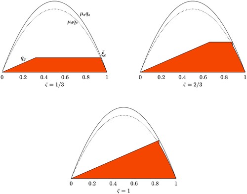
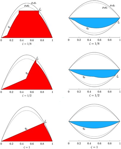
4.2.1. Case I: $|{\sigma }_y|<\frac{3}{2}\left({\mu }_s{F}_z/C_{y\alpha }\right)$

This case corresponds to have a small lateral slip. In steady-state conditions, the breakaway point is thus always located on the same side of the trailing edge (see Figure 2). Owing the previous assumptions, the solutions for the lateral deformation of the bristle in the adhesion length read (27) $u_y^a(\xi ,\varsigma )=\{\begin{array}{ll}{u}_y^{-}\left(\xi \right)={\sigma }_y\xi & 0\le \xi <\varsigma \\ u_y^{+}\left(\varsigma \right)={\sigma }_y\varsigma & \xi \ge \varsigma \end{array},$(27) Here the problem is one-dimensional and very straightforward. In particular, it is worth to highlight that the force is linear with slope ${\sigma }_y$ between $0\le \xi <\varsigma$, constant in the region $\varsigma \le \xi <{\xi }_c$ – where ${\xi }_c$ identifies the position of the breakaway point – and then it follows the trend of the dynamic friction parabola ${\mu }_d{q}_z\left(\xi \right)$ after the drop from the static friction one ${\mu }_s{q}_z\left(\xi \right)$, according to (28) $u_y^s\left(\xi \right)=-\frac{{\mu }_d}{k_y}{q}_z\left(\xi \right)\mathrm{s}\mathrm{i}\mathrm{g}\mathrm{n}\left(V_{sy}\right)=\frac{{\mu }_d}{k_y}{q}_z\left(\xi \right)\mathrm{s}\mathrm{i}\mathrm{g}\mathrm{n}\left({\sigma }_y\right).$(28) (29a) $\begin{array}{rl}{\xi }_c\left(\varsigma \right)& =\frac{l}{2}+\sqrt{\frac{l^2}{4}-\frac{C_{y\alpha }|{\sigma }_y|l\varsigma }{3{\mu }_s{F}_z}}⟺\varsigma <l(1-\frac{C_{y\alpha }}{3{\mu }_s{F}_z}|{\sigma }_y|),\end{array}$(29a) (29b) $\begin{array}{rl}{\xi }_c\left(\varsigma \right)& =l(1-\frac{C_{y\alpha }}{3{\mu }_s{F}_z}|{\sigma }_y|)⟺\varsigma \ge l(1-\frac{C_{y\alpha }}{3{\mu }_s{F}_z}|{\sigma }_y|),\end{array}$(29b) with $C_{y\alpha }:=k_{y}w{l}^2/2$. It must be emphasised that, for $\varsigma =l(1-C_{y\alpha }|{\sigma }_y|/(3{\mu }_s{F}_z\left)\right)$, the two solutions (29a(29a) $\begin{array}{rl}{\xi }_c\left(\varsigma \right)& =\frac{l}{2}+\sqrt{\frac{l^2}{4}-\frac{C_{y\alpha }|{\sigma }_y|l\varsigma }{3{\mu }_s{F}_z}}⟺\varsigma <l(1-\frac{C_{y\alpha }}{3{\mu }_s{F}_z}|{\sigma }_y|),\end{array}$(29a) ) and (29b(29b) $\begin{array}{rl}{\xi }_c\left(\varsigma \right)& =l(1-\frac{C_{y\alpha }}{3{\mu }_s{F}_z}|{\sigma }_y|)⟺\varsigma \ge l(1-\frac{C_{y\alpha }}{3{\mu }_s{F}_z}|{\sigma }_y|),\end{array}$(29b) ) coincide. Furthermore, we can have an estimate of the relaxation length and time due to the bristle dynamics, since the steady-state conditions are reached when the following relation is satisfied (30) ${\varsigma }^{\ast }=l(1-\frac{C_{y\alpha }}{3{\mu }_s{F}_z}|{\sigma }_y|)=l(1-\frac{C_{y\alpha }}{3{\mu }_s{F}_z}\frac{|V_{sy}|}{V_r}),$(30) which can be rearranged in the form (31) $t^{\ast }=\frac{l}{V_r}-\frac{C_{y\alpha }l}{3{\mu }_s{F}_z}\frac{|V_{sy}|}{V_r^2}$(31) where with $t^{\ast }$ we denoted the relaxation time. Equations (30(30) ${\varsigma }^{\ast }=l(1-\frac{C_{y\alpha }}{3{\mu }_s{F}_z}|{\sigma }_y|)=l(1-\frac{C_{y\alpha }}{3{\mu }_s{F}_z}\frac{|V_{sy}|}{V_r}),$(30) ) and (31(31) $t^{\ast }=\frac{l}{V_r}-\frac{C_{y\alpha }l}{3{\mu }_s{F}_z}\frac{|V_{sy}|}{V_r^2}$(31) ) state that the relaxation length and time vary linearly and quadratically with the inverse power of the rolling speed, respectively, and are both proportional to the macro-sliding speed.

Figure 2. Time trend for the shear stresses $q_y(\xi ,\varsigma )$ in the contact patch for case I. The three figures refer to different values of the nondimensional travelled distance $\overline{\varsigma }$. Since the trend for the solution $u_y^{+}\left(\varsigma \right)$ in the adhesion region is constant, the steady-state condition is reached when $\overline{\varsigma }=1$, or, equivalently, when the travelled distance equals the contact length.

Finally, integrating over the contact patch, the total lateral force $F_{y\alpha }\left(\varsigma \right)$ is as follows (32) $F_{y\alpha }\left(\varsigma \right)=\{\begin{array}{ll}{\displaystyle w{k}_y\left({\int }_0^{\varsigma }{u}_y^{-}\right(\xi )\mathrm{d}\xi +{\int }_{\varsigma }^{{\xi }_c}{u}_y^{+}(\varsigma )\mathrm{d}\xi +{\int }_{{\xi }_c}^l{u}_y^s(\xi \left)\mathrm{d}\xi \right)}& 0\le \varsigma <{\xi }_c\\ {\displaystyle w{k}_y\left({\int }_0^{{\xi }_c}{u}_y^{-}\right(\xi )\mathrm{d}\xi +{\int }_{{\xi }_c}^l{u}_y^s(\xi \left)\mathrm{d}\xi \right)}& \varsigma \ge {\xi }_c\end{array},$(32) and the and the self-aligning moment $M_z\left(\varsigma \right)$ reads (33) $M_z\left(\varsigma \right)=\frac{1}{2}wl{k}_y{\int }_0^l{u}_y(\xi ,\varsigma )\mathrm{d}\xi -w{k}_y{\int }_0^l{u}_y(\xi ,\varsigma )\xi \mathrm{d}\xi =\frac{l}{2}{F}_{y\alpha }\left(\varsigma \right)-J\left(\varsigma \right),$(33) with $J\left(\varsigma \right)$ defined as (34) $J\left(\varsigma \right)=\{\begin{array}{ll}{\displaystyle w{k}_y\left({\int }_0^{\varsigma }{u}_y^{-}\right(\xi )\xi \mathrm{d}\xi +{\int }_{\varsigma }^{{\xi }_c}{u}_y^{+}(\varsigma )\xi \mathrm{d}\xi +{\int }_{{\xi }_c}^l{u}_y^s(\xi \left)\xi \mathrm{d}\xi \right)}& 0\le \varsigma <{\xi }_c\\ {\displaystyle w{k}_y\left({\int }_0^{{\xi }_c}{u}_y^{-}\right(\xi )\xi \mathrm{d}\xi +{\int }_{{\xi }_c}^l{u}_y^s(\xi \left)\xi \mathrm{d}\xi \right)}& \varsigma \ge {\xi }_c\end{array}.$(34) The final formulae are (35) $\begin{array}{rl}{F}_{y\alpha }\left(\varsigma \right)& =\{\begin{array}{ll}{\displaystyle \frac{C_{y\alpha }}{l^2}{\sigma }_y\varsigma (2{\xi }_c-\varsigma )+{\mu }_d\frac{6F_z}{l^2}(\frac{l^2}{6}-\frac{{\xi }_c^2}{2}+\frac{{\xi }_c^3}{3l})\mathrm{s}\mathrm{i}\mathrm{g}\mathrm{n}\left({\sigma }_y\right)}& 0\le \varsigma <{\xi }_c\\ {\displaystyle \frac{C_{y\alpha }}{l^2}{\sigma }_y{\xi }_c^2+{\mu }_d\frac{6F_z}{l^2}(\frac{l^2}{6}-\frac{{\xi }_c^2}{2}+\frac{{\xi }_c^3}{3l})\mathrm{s}\mathrm{i}\mathrm{g}\mathrm{n}\left({\sigma }_y\right)}& \varsigma \ge {\xi }_c\end{array},\end{array}$(35) (36) $\begin{array}{rl}J\left(\varsigma \right)& =\{\begin{array}{ll}{\displaystyle \frac{C_{y\alpha }}{3l^2}{\sigma }_y\varsigma (3{\xi }_c^2-{\varsigma }^2)+{\mu }_d\frac{6F_z}{l^2}(\frac{l^3}{12}-\frac{{\xi }_c^3}{4}+\frac{{\xi }_c^4}{4l})\mathrm{s}\mathrm{i}\mathrm{g}\mathrm{n}\left({\sigma }_y\right)}& 0\le \varsigma <{\xi }_c\\ {\displaystyle \frac{C_{y\alpha }}{3l^2}{\sigma }_y{\xi }_c^3+{\mu }_d\frac{6F_z}{l^2}(\frac{l^3}{12}-\frac{{\xi }_c^3}{4}+\frac{{\xi }_c^4}{4l})\mathrm{s}\mathrm{i}\mathrm{g}\mathrm{n}\left({\sigma }_y\right)}& \varsigma \ge {\xi }_c\end{array},\end{array}$(36) where ${\xi }_c\left(\varsigma \right)$ is given by (29a(29a) $\begin{array}{rl}{\xi }_c\left(\varsigma \right)& =\frac{l}{2}+\sqrt{\frac{l^2}{4}-\frac{C_{y\alpha }|{\sigma }_y|l\varsigma }{3{\mu }_s{F}_z}}⟺\varsigma <l(1-\frac{C_{y\alpha }}{3{\mu }_s{F}_z}|{\sigma }_y|),\end{array}$(29a) ) and (29b(29b) $\begin{array}{rl}{\xi }_c\left(\varsigma \right)& =l(1-\frac{C_{y\alpha }}{3{\mu }_s{F}_z}|{\sigma }_y|)⟺\varsigma \ge l(1-\frac{C_{y\alpha }}{3{\mu }_s{F}_z}|{\sigma }_y|),\end{array}$(29b) ), respectively. Note that, for $\varsigma \ge {\xi }_c\left(\varsigma \right)$, it is also (37) $F_{y\alpha }=C_{y\alpha }|{\sigma }_y|[1-(2-\frac{{\mu }_d}{{\mu }_s})\frac{C_{y\alpha }|{\sigma }_y|}{3{\mu }_s{F}_z}+(3-2\frac{{\mu }_d}{{\mu }_s})\frac{{\left(C_{y\alpha }|{\sigma }_y|\right)}^2}{27({\mu }_s{F}_z{)}^2}]\mathrm{s}\mathrm{i}\mathrm{g}\mathrm{n}\left({\sigma }_y\right).$(37) which is the well-known steady-state formula for $F_{y\alpha }$ in the case of parabolic pressure distribution.

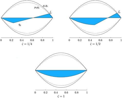
4.2.2. Case II: $\frac{3}{2}\left({\mu }_s{F}_z/C_{y\alpha }\right)\le |{\sigma }_y|<\left(3{\mu }_s{F}_z/C_{y\alpha }\right)$

In this case, we have high lateral slip, but still smaller than the critical value ${\sigma }_y^{crit}=3{\mu }_s{F}_z/C_{y\alpha }$. In steady-state conditions, the breakaway point is located on the same side of the leading edge. There are three different solutions depending on the travelled distance, as shown in Figure 3.

Figure 3. Time trend for the shear stresses $q_y(\xi ,\varsigma )$ in the contact patch for case II. The three figures refer to different values of the nondimensional travelled distance $\overline{\varsigma }$. Since the trend for the solution $u_y^{+}\left(\varsigma \right)$ in the adhesion region is constant, the steady-state condition is reached when $\overline{\varsigma }=\frac{3}{4}\left({\mu }_s{F}_z/C_{y\alpha }|{\sigma }_y|\right)$, or, equivalently, when the travelled distance equals the value ${\varsigma }^{\ast }$.

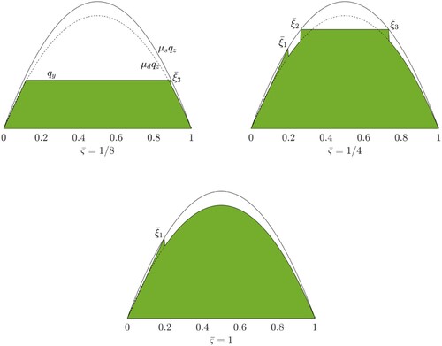
We denote with (38a) $\begin{array}{rl}{\xi }_1& =l(1-\frac{C_{y\alpha }}{3{\mu }_s{F}_z}|{\sigma }_y|),\end{array}$(38a) (38b) $\begin{array}{rl}{\xi }_2\left(\varsigma \right)& =\frac{l}{2}-\sqrt{\frac{l^2}{4}-\frac{C_{y\alpha }|{\sigma }_y|l\varsigma }{3{\mu }_s{F}_z}},\end{array}$(38b) (38c) $\begin{array}{rl}{\xi }_3\left(\varsigma \right)& =\frac{l}{2}+\sqrt{\frac{l^2}{4}-\frac{C_{y\alpha }|{\sigma }_y|l\varsigma }{3{\mu }_s{F}_z}},\end{array}$(38c) (38d) $\begin{array}{rl}{\varsigma }^{\ast }& =\frac{3}{4}\frac{l{\mu }_s{F}_z}{C_{y\alpha }|{\sigma }_y|},\end{array}$(38d) so that the lateral force and the quantity $J\left(\varsigma \right)$ can be written as (39) $\begin{array}{rl}{F}_{y\alpha }\left(\varsigma \right)& =\{\begin{array}{ll}{\displaystyle w{k}_y\left({\int }_0^{\varsigma }{u}_y^{-}\right(\xi )\mathrm{d}\xi +{\int }_{\varsigma }^{{\xi }_3}{u}_y^{+}(\varsigma )\mathrm{d}\xi +{\int }_{{\xi }_3}^l{u}_y^s(\xi \left)\mathrm{d}\xi \right)}& 0\le \varsigma <{\xi }_1\\ {\displaystyle w{k}_y\left({\int }_0^{{\xi }_1}{u}_y^{-}\right(\xi )\mathrm{d}\xi +{\int }_{{\xi }_1}^{{\xi }_2}{u}_y^s(\xi )\mathrm{d}\xi }\\ {\displaystyle +{\int }_{{\xi }_2}^{{\xi }_3}{u}_y^{+}\left(\varsigma \right)\mathrm{d}\xi +{\int }_{{\xi }_3}^l{u}_y^s\left(\xi \right)\mathrm{d}\xi )}& {\xi }_1\le \varsigma <{\varsigma }^{\ast }\\ {\displaystyle w{k}_y\left({\int }_0^{{\xi }_1}{u}_y^{-}\right(\xi )\mathrm{d}\xi +{\int }_{{\xi }_1}^l{u}_y^s(\xi \left)\mathrm{d}\xi \right)}& \varsigma \ge {\varsigma }^{\ast }\end{array},\end{array}$(39) (40) $\begin{array}{rl}J\left(\varsigma \right)& =\{\begin{array}{ll}{\displaystyle w{k}_y\left({\int }_0^{\varsigma }{u}_y^{-}\right(\xi )\xi \mathrm{d}\xi +{\int }_{\varsigma }^{{\xi }_3}{u}_y^{+}(\varsigma )\xi \mathrm{d}\xi +{\int }_{{\xi }_3}^l{u}_y^s(\xi \left)\xi \mathrm{d}\xi \right)}& 0\le \varsigma <{\xi }_1\\ {\displaystyle w{k}_y\left({\int }_0^{{\xi }_1}{u}_y^{-}\right(\xi )\xi \mathrm{d}\xi +{\int }_{{\xi }_1}^{{\xi }_2}{u}_y^s(\xi )\xi \mathrm{d}\xi }\\ {\displaystyle +{\int }_{{\xi }_2}^{{\xi }_3}{u}_y^{+}\left(\varsigma \right)\xi \mathrm{d}\xi +{\int }_{{\xi }_3}^l{u}_y^s\left(\xi \right)\xi \mathrm{d}\xi )}& {\xi }_1\le \varsigma <{\varsigma }^{\ast }\\ {\displaystyle w{k}_y\left({\int }_0^{{\xi }_1}{u}_y^{(}\xi \right)-\xi \mathrm{d}\xi +{\int }_{{\xi }_1}^l{u}_y^s\left(\xi \right)\xi \mathrm{d}\xi )}& \varsigma \ge {\varsigma }^{\ast }\end{array}.\end{array}$(40) Integrating over the contact length provides, respectively (41) $F_{y\alpha }\left(\varsigma \right)=\{\begin{array}{ll}{\displaystyle \frac{C_{y\alpha }}{l^2}{\sigma }_y\varsigma (2{\xi }_3-\varsigma )+{\mu }_d\frac{6F_z}{l^2}(\frac{l^2}{6}-\frac{{\xi }_3^2}{2}+\frac{{\xi }_3^3}{3l})\mathrm{s}\mathrm{i}\mathrm{g}\mathrm{n}\left({\sigma }_y\right)}& 0\le \varsigma <{\xi }_1\\ {\displaystyle \frac{C_{y\alpha }}{l^2}{\sigma }_y[{\xi }_1^2+2\varsigma ({\xi }_3-{\xi }_2\left)\right]}\\ {\displaystyle +{\mu }_d\frac{6F_z}{l^2}(\frac{l^2}{6}-\frac{{\xi }_1^2-{\xi }_2^2+{\xi }_3^2}{2}+\frac{{\xi }_1^3-{\xi }_2^3+{\xi }_3^3}{3l})\mathrm{s}\mathrm{i}\mathrm{g}\mathrm{n}\left({\sigma }_y\right)}& {\xi }_1\le \varsigma <{\varsigma }^{\ast }\\ {\displaystyle \frac{C_{y\alpha }}{l^2}{\sigma }_y{\xi }_1^2+{\mu }_d\frac{6F_z}{l^2}(\frac{l^2}{6}-\frac{{\xi }_1^2}{2}+\frac{{\xi }_1^3}{3l})\mathrm{s}\mathrm{i}\mathrm{g}\mathrm{n}\left({\sigma }_y\right)}& \varsigma \ge {\varsigma }^{\ast }\end{array},$(41) and (42) $J\left(\varsigma \right)=\{\begin{array}{ll}{\displaystyle \frac{C_{y\alpha }}{3l^2}{\sigma }_y\varsigma (3{\xi }_3^2-{\varsigma }^2)+{\mu }_d\frac{6F_z}{l^2}(\frac{l^3}{12}-\frac{{\xi }_3^3}{3}+\frac{{\xi }_3^4}{3l})\mathrm{s}\mathrm{i}\mathrm{g}\mathrm{n}\left({\sigma }_y\right)}& 0\le \varsigma <{\xi }_1\\ {\displaystyle \frac{C_{y\alpha }}{3l^2}{\sigma }_y[{\xi }_1^3+3\varsigma ({\xi }_3^2-{\xi }_2^2\left)\right]}\\ {\displaystyle +{\mu }_d\frac{6F_z}{l^2}(\frac{l^3}{12}-\frac{{\xi }_1^3-{\xi }_2^3+{\xi }_3^3}{3}+\frac{{\xi }_1^4-{\xi }_2^4+{\xi }_3^4}{4l})\mathrm{s}\mathrm{i}\mathrm{g}\mathrm{n}\left({\sigma }_y\right)}& {\xi }_1\le \varsigma <{\varsigma }^{\ast }\\ {\displaystyle \frac{C_{y\alpha }}{3l^2}{\sigma }_y{\xi }_1^3+{\mu }_d\frac{6F_z}{l^2}(\frac{l^3}{12}-\frac{{\xi }_1^3}{3}+\frac{{\xi }_1^4}{4l})\mathrm{s}\mathrm{i}\mathrm{g}\mathrm{n}\left({\sigma }_y\right)}& \varsigma \ge {\varsigma }^{\ast }\end{array}.$(42) Note that the above equations state that, when the travelled distance is between ${\xi }_1$ and ${\varsigma }^{\ast }$, there are two sliding regions. Indeed, from the point ${\xi }_1$ to ${\xi }_2\left(\varsigma \right)$, the vertical pressure cannot supply the bristles with enough adhesion power, and they start sliding within the contact patch; however, from ${\xi }_2\left(\varsigma \right)$ to ${\xi }_3\left(\varsigma \right)$, the friction force required to stick to the ground is constant and less than the maximum force available: this brings about a sudden discontinuity in the bristle deformation. This result can appear a bit counterintuitive, but it is worth to remark that the bristles behave independently of each other. Furthermore, a rigorous proof is given in Appendix 1. Then, when the travelled distance is greater than ${\varsigma }^{\ast }$, the deformation $u_y^{+}\left(\varsigma \right)$ required to the bristles to adhere to the road is always greater than the peak value of the static pressure distribution, and sliding occurs starting from the breakaway point ${\xi }_1$ corresponding to the steady-state solution.

4.2.3. Case III: $|{\sigma }_y|\ge 3{\mu }_s{F}_z/C_{y\alpha }$

This situation corresponds to have total sliding within the whole contact patch in steady-state condition, since the slip value ${\sigma }_y$ is greater than the critical one. However, during the transient, a small portion of the contact patch can be still characterised by adhesion condition if the travelled distance is smaller than ${\varsigma }^{\ast }$, as shown in Figure 4.

Figure 4. Time trend for the shear stresses $q_y(\xi ,\varsigma )$ in the contact patch for case III. The three figures refer to different values of the nondimensional travelled distance $\overline{\varsigma }$. Since the trend for the solution $u_y^{+}\left(\varsigma \right)$ in the adhesion region is constant, the steady-state condition is reached when $\overline{\varsigma }=\frac{3}{4}\left({\mu }_s{F}_z/C_{y\alpha }|{\sigma }_y|\right)$, or, equivalently, when the travelled distance equals the value ${\varsigma }^{\ast }$.

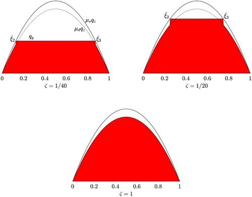
Indeed, in this case, in the area between ${\xi }_2\left(\varsigma \right)$ and ${\xi }_3\left(\varsigma \right)$, the deformation of the bristles read $u_y^{+}\left(\varsigma \right)$, and the friction force needed to stick the road can be lower than the maximum adhesive power available. Hence, this scenario can be seen as a special case of II, with ${\xi }_1=0$.

4.3. Pure camber

The bristle displacement due to pure camber has a component along both the axes, as stated by Equations (19(19a) $\begin{array}{rl}{u}_x^{-}(\mathit{\xi },t)& =-\frac{V_{sx}}{V_r}\xi +\frac{{\omega }_z}{V_r}\xi \eta +d_x(t-\frac{\xi }{V_r})-d_x\left(t\right),\end{array}$(19a) ) and (20(20a) $\begin{array}{rl}{u}_x^{+}(\mathit{\xi },t)& =-V_{sx}t+{\omega }_z\eta t+d_x\left(0\right)-d_x\left(t\right)+u_x^0(\xi -V_{r}t),\end{array}$(20a) ). In this case, the problem is never one-dimensional, even though it is common to neglect the deformation $u_x(\mathit{\xi },\varsigma )$. Indeed, whilst the displacement along the x direction is linear and small in value, the one along the $\eta =y$ coordinate is parabolic in ξ and also independent on the lateral position of the bristle. Hence, in the following analysis, we only focus on the y component of the deformation. Furthermore, we assume to have no steering and small camber angle, so that $\phi =\sin \gamma \simeq \gamma$.

In this case, the different solutions inside the contact patch read, respectively (43) $u_y^a(\xi ,\varsigma )=\{\begin{array}{ll}{\displaystyle u_y^{-}\left(\xi \right)=\frac{\gamma }{2R_r}\xi (l-\xi )}& 0\le \xi <\varsigma \\ {\displaystyle u_y^{+}(\xi ,\varsigma )=\frac{\gamma }{2R_r}\varsigma (l-2\xi +\varsigma )}& \xi \ge \varsigma \end{array},$(43) in the adhesion region and (44) $u_y^s\left(\xi \right)=-\frac{{\mu }_d}{k_y}{q}_z\left(\xi \right)\mathrm{s}\mathrm{i}\mathrm{g}\mathrm{n}\left(\gamma \right)$(44) in the sliding portion of the contact patch.

Since the spin causes a parabolic deformation, the breakaway point – in steady-state conditions – always coincides with the leading or the trailing edge of the contact patch. However, the first case is not of interest, since the spin speed is always very small and can be often neglected. So, we only consider the second scenario. During the transient, the solution $u_y^{+}(\xi ,\varsigma )$ is linear in ξ and the its slope is always opposite to the sign of the spin parameter (Figure 5). Furthermore, the slope increases in absolute value with the time or, equivalently, with the travelled distance ς. It can be noted that, for $\varsigma >0$, $u_y^{+}(\xi ,\varsigma )$ always changes sign in $\xi =(l+\varsigma )/2$, hence the negative sign in Equation (44(44) $u_y^s\left(\xi \right)=-\frac{{\mu }_d}{k_y}{q}_z\left(\xi \right)\mathrm{s}\mathrm{i}\mathrm{g}\mathrm{n}\left(\gamma \right)$(44) ).

Figure 5. Time trend for the shear stresses $q_y(\xi ,\varsigma )$ in the contact patch due to pure camber. The three figures refer to different values of the nondimensional travelled distance $\overline{\varsigma }$. Since the trends for the solutions $u_y^{-}\left(\xi \right)$ and $u_y^{+}(\xi ,\varsigma )$ in the adhesion region are parabolic and linear, respectively, the steady-state condition is only reached when $\overline{\varsigma }$ = 1, or, equivalently, when the travelled distance equals the contact length.

From the previous observations, it is clear that, during the transient, it is only possible to have one breakaway point, which is always located on the same side of the trailing edge. More specifically, its position reads as follows (45) ${\xi }_c\left(\varsigma \right)=\frac{l}{2}-\frac{C_{y\gamma }}{{\mu }_s{F}_z}|\gamma |\varsigma +\sqrt{{(\frac{l}{2}-\frac{C_{y\gamma }}{{\mu }_s{F}_z}|\gamma |\varsigma )}^2+\frac{C_{y\gamma }}{{\mu }_s{F}_z}|\gamma |\varsigma (l+\varsigma )}⟺\varsigma <l,$(45) where we defined $C_{y\gamma }$ as (46) $C_{y\gamma }:=\frac{1}{6}{k}_{y}w\frac{l^3}{2R_r}.$(46) It is worth to note that, in case of pure spin, the relaxation length almost coincides with the length of the contact patch.

Integrating over the contact length, it is possible to deduce the value of the lateral force $F_{y\gamma }\left(\varsigma \right)$ (47) $F_{y\gamma }\left(\varsigma \right)=\{\begin{array}{ll}{\displaystyle w{k}_y\left({\int }_0^{\varsigma }{u}_y^{-}\right(\xi )\mathrm{d}\xi +{\int }_{\varsigma }^{{\xi }_c}{u}_y^{+}(\xi ,\varsigma )\mathrm{d}\xi +{\int }_{{\xi }_c}^l{u}_y^s(\xi \left)\mathrm{d}\xi \right)}& 0\le \varsigma <l\\ {\displaystyle w{k}_y{\int }_0^l{u}_y^{-}\left(\xi \right)\mathrm{d}\xi }& \varsigma \ge l\end{array},$(47) which gives (48) $F_{y\gamma }\left(\varsigma \right)=\{\begin{array}{l}{\displaystyle \frac{C_{y\gamma }}{l^3}\gamma \varsigma \left[6{\xi }_c\right(l-{\xi }_c+\varsigma )-\varsigma (3l+2s\left)\right]}\\ -{\displaystyle {\mu }_d\frac{6F_z}{l^2}(\frac{l^2}{6}-\frac{{\xi }_c^2}{2}+\frac{{\xi }_c^3}{3l})\mathrm{s}\mathrm{i}\mathrm{g}\mathrm{n}\left(\gamma \right)}& 0\le \varsigma <l\\ C_{y\gamma }\gamma & \varsigma \ge l\end{array}.$(48)

4.4. Qualitative analysis for nonzero initial condition

The preceding investigation was based on the assumption of zero initial condition, i.e. ${\mathit{u}}_t^0=\mathbf{0}$. When the bristles are already deformed before the transient takes place, a quantitative analysis becomes more challenging. Hence, we may limit ourselves to some qualitative considerations about the time trend of the shear stresses in the contact patch.

Referring to the pure lateral case, the initial condition $u_y^0$ propagates along the steady-state solution with the same travelling speed $V_r$. The steady-state solution is again reached when the travelled distance ς equals the steady-state position of the breakaway point.

Figure 6 (left-hand side panel) shows the time trend of the sear stresses when starting from unsteady-state conditions with an initial value ${\sigma }_y^0$ greater than the critical one. It can be noted that, if the slip had been kept to its original value ${\sigma }_y^0$, total sliding had been occurred inside the contact patch after a whilst. Instead, since the new value ${\sigma }_y$ is smaller than the critical one, its introduction prevents the the tyre from sliding fully.

Figure 6. Time trend for the shear stresses $q_y(\xi ,\varsigma )$ in the contact patch due to pure lateral interaction and pure camber, respectively, starting from nonzero initial conditions $u_y^0\ne 0$. The figures refer to different values of the nondimensional travelled distance $\overline{\varsigma }$. The initial condition for the pure lateral case (left-hand side panel) corresponds to a transient trend for the deformation of the bristles due to an initial slip value ${\sigma }_y^0>{\sigma }_y^{crit}$. The transient solution for the camber (right-hand side panel) refers to a case in which the initial spin value ${\gamma }^0$ has the same sign as the current one. The initial condition corresponds to a steady-state trend of the bristle displacement.

Finally, the transient trend due to variation in the camber angle are depicted in the right-hand side panel of Figure 6. The relaxation again equals the contact patch length, since the camber causes a parabolic distribution of the deformations.

5. Two-regime tyre formulae

5.1. General procedure

As shown previously, an analytical formulation for the tyre characteristics can be derived for different cases. However, it is too complicated to be used in vehicle dynamics simulations. Furthermore, neglecting the carcass compliance allows for some simplifications, but limits the practical relevance of the analysis. The aim is hence to develop a class of simplified Two-Regime Tyre Formulae (TRF) interpolating between two different regimes of low and high rolling speed. The TRF family must be able to macroscopically represent the phenomena due to the transient of the bristle whilst also including the dynamics of the tyre carcass.

First, we introduce the augmented vectors for the generalised forces, displacements, velocities and slips, defined as (49a) $\begin{array}{rl}{\mathit{F}}_t^{\star }& :=\left[\begin{array}{c}{\mathit{F}}_t\\ M_z\end{array}\right],\end{array}$(49a) (49b) $\begin{array}{rl}{\mathit{d}}^{\star }& :=\left[\begin{array}{c}\mathit{d}\\ 0\end{array}\right],\end{array}$(49b) (49c) $\begin{array}{rl}{\mathit{V}}_s^{\star }& :=\left[\begin{array}{c}{\mathit{V}}_s\\ {\omega }_z\end{array}\right],\end{array}$(49c) (49d) $\begin{array}{rl}{\mathit{\sigma }}^{\star }& :=-\frac{{\mathit{V}}_s^{\star }}{V_r}=\left[\begin{array}{c}\mathit{\sigma }\\ \phi R_r\end{array}\right].\end{array}$(49d) Then, as already mentioned, we remark that, for $V_r\to 0$, Equation (20(20a) $\begin{array}{rl}{u}_x^{+}(\mathit{\xi },t)& =-V_{sx}t+{\omega }_z\eta t+d_x\left(0\right)-d_x\left(t\right)+u_x^0(\xi -V_{r}t),\end{array}$(20a) ) turns into a time integrator. Thus, at low rolling speed, we can approximate (50) ${\mathit{F}}_t^{\star }\simeq {\mathit{F}}_1^{\star }({\mathit{S}}_s^{\star },{\mathit{d}}^{\star }),$(50) where we denoted with ${\mathit{S}}_s^{\star }$ the primitive function of ${\mathit{V}}_{s,low}^{\star }$ at low rolling speed. Differentiating (50(50) ${\mathit{F}}_t^{\star }\simeq {\mathit{F}}_1^{\star }({\mathit{S}}_s^{\star },{\mathit{d}}^{\star }),$(50) ) results finally in (51) ${\dot{\mathit{F}}}_t^{\star }\simeq {\dot{\mathit{F}}}_t^{\star }({\mathit{S}}_s^{\star },{\mathit{V}}_{s,low},{\mathit{d}}^{\star },{\dot{\mathit{d}}}^{\star }).$(51) On the other hand, at high rolling speed, we can neglect the partial derivative taken with respect to the time in Equation (13(13a) $\begin{array}{rl}\frac{\mathrm{\partial }{u}_x(\mathit{\xi },t)}{\mathrm{\partial }t}+V_r\left(t\right)\frac{\mathrm{\partial }{u}_x(\mathit{\xi },t)}{\mathrm{\partial }\xi }& =-V_{sx}\left(t\right)+{\omega }_z\left(t\right)\eta -{\dot{d}}_x\left(t\right),\end{array}$(13a) ) and express the generalised tangential forces as a function of the slip quantities and the tyre carcass displacement and speed, according to (52) ${\mathit{F}}_t^{\star }\simeq {\mathit{F}}_2^{\ast }({\mathit{\sigma }}^{\star },\mathit{d},\dot{\mathit{d}})={\mathit{F}}_2^{\star }(-\frac{{\mathit{V}}_{s,high}^{\star }}{V_r},\frac{{\mathit{d}}^{\star }}{V_r},\frac{{\dot{\mathit{d}}}^{\star }}{V_r}).$(52) Since it is also (53a) $\begin{array}{rl}{\dot{\mathit{F}}}_t& ={\mathbf{C}}^{\mathrm{\prime }}\dot{\mathit{d}},\end{array}$(53a) (53b) $\begin{array}{rl}{\mathit{F}}_t& ={\mathbf{C}}^{\mathrm{\prime }}\mathit{d},\end{array}$(53b) we can recast Equations (51(51) ${\dot{\mathit{F}}}_t^{\star }\simeq {\dot{\mathit{F}}}_t^{\star }({\mathit{S}}_s^{\star },{\mathit{V}}_{s,low},{\mathit{d}}^{\star },{\dot{\mathit{d}}}^{\star }).$(51) ) and (52(52) ${\mathit{F}}_t^{\star }\simeq {\mathit{F}}_2^{\ast }({\mathit{\sigma }}^{\star },\mathit{d},\dot{\mathit{d}})={\mathit{F}}_2^{\star }(-\frac{{\mathit{V}}_{s,high}^{\star }}{V_r},\frac{{\mathit{d}}^{\star }}{V_r},\frac{{\dot{\mathit{d}}}^{\star }}{V_r}).$(52) ) as (54a) $\begin{array}{rl}{\dot{\mathit{F}}}_t^{\star }& \simeq {\mathit{F}}_1({\mathit{S}}_s^{\star },{\mathit{V}}_{s,low}^{\star },\mathbf{\Gamma }{\mathit{F}}_t^{\star },\mathbf{\Gamma }{\dot{\mathit{F}}}_t^{\star }),\end{array}$(54a) (54b) $\begin{array}{rl}{\mathit{F}}_t^{\star }& \simeq {\mathit{F}}_2(-\frac{{\mathit{V}}_{s,high}^{\star }}{V_r},\frac{\mathbf{\Gamma }{\mathit{F}}_t^{\ast }}{V_r},\frac{\mathbf{\Gamma }{\dot{\mathit{F}}}_t^{\star }}{V_r}),\end{array}$(54b) where the matrix $\mathbf{\Gamma }$ is defined as (55) $\mathbf{\Gamma }:=\left[\begin{array}{cc}{\mathbf{C}}^{{}^{\prime }-1}& \mathbf{0}\\ \mathbf{0}& 0\end{array}\right].$(55) Recasting (54(54a) $\begin{array}{rl}{\dot{\mathit{F}}}_t^{\star }& \simeq {\mathit{F}}_1({\mathit{S}}_s^{\star },{\mathit{V}}_{s,low}^{\star },\mathbf{\Gamma }{\mathit{F}}_t^{\star },\mathbf{\Gamma }{\dot{\mathit{F}}}_t^{\star }),\end{array}$(54a) ) in implicit form as (56a) $\begin{array}{rl}{\mathit{H}}_1({\mathit{S}}_s^{\star },{\mathit{V}}_{s,low}^{\star },{\mathit{F}}_t^{\star },{\dot{\mathit{F}}}_t^{\star })& ={\dot{\mathit{F}}}_t^{\star }-{\mathit{F}}_1({\mathit{S}}_s^{\star },{\mathit{V}}_{s,low}^{\star },\mathbf{\Gamma }{\mathit{F}}_t^{\star },\mathbf{\Gamma }{\dot{\mathit{F}}}_t^{\star })=\mathbf{0},\end{array}$(56a) (56b) $\begin{array}{rl}{\mathit{H}}_2({\mathit{V}}_{s,high}^{\star },{\mathit{F}}_t^{\star },{\dot{\mathit{F}}}_t^{\star },V_r)& ={\mathit{F}}_t^{\star }-{\mathit{F}}_2(-\frac{{\mathit{V}}_{s,high}^{\star }}{V_r},\frac{\mathbf{\Gamma }{\mathit{F}}_t^{\star }}{V_r},\frac{\mathbf{\Gamma }{\dot{\mathit{F}}}_t^{\star }}{V_r})=\mathbf{0},\end{array}$(56b) it is possible to locally express the variables ${\mathit{V}}_{s,low}^{\star }$ and ${\mathit{V}}_{s,high}^{\star }$ according to the Implicit Function Theorem, obtaining (57a) $\begin{array}{rl}{\mathit{V}}_{s,low}^{\star }& ={\mathbf{\Sigma }}_1({\mathit{S}}_s^{\star },{\mathit{F}}_t^{\star },{\dot{\mathit{F}}}_t^{\star }),\end{array}$(57a) (57b) $\begin{array}{rl}{\mathit{V}}_{s,high}^{\star }& =V_r{\mathbf{\Sigma }}_2({\mathit{F}}_t^{\star },{\dot{\mathit{F}}}_t^{\star }),\end{array}$(57b) in which we call ${\mathbf{\Sigma }}_1=\left[{\mathrm{\Sigma }}_{1x}\right(\bullet \left){\mathrm{\Sigma }}_{1y}\right(\bullet \left){\mathrm{\Sigma }}_{1z}\right(\bullet ){]}^T$ and ${\mathbf{\Sigma }}_2=\left[{\mathrm{\Sigma }}_{2x}\right(\bullet \left){\mathrm{\Sigma }}_{2y}\right(\bullet \left){\mathrm{\Sigma }}_{2z}\right(\bullet ){]}^T$ Sigma Functions. It is worth to point out that (57a(57a) $\begin{array}{rl}{\mathit{V}}_{s,low}^{\star }& ={\mathbf{\Sigma }}_1({\mathit{S}}_s^{\star },{\mathit{F}}_t^{\star },{\dot{\mathit{F}}}_t^{\star }),\end{array}$(57a) ) and (57b(57b) $\begin{array}{rl}{\mathit{V}}_{s,high}^{\star }& =V_r{\mathbf{\Sigma }}_2({\mathit{F}}_t^{\star },{\dot{\mathit{F}}}_t^{\star }),\end{array}$(57b) ) are valid for low and high rolling speeds $V_r$, respectively, and constitute a set of integro-differential equations.

However, they can be further simplified by introducing additional assumptions. Indeed, if the contact patch is not parametrised as a function of the time, the integral quantities and the carcass displacement disappear in (51(51) ${\dot{\mathit{F}}}_t^{\star }\simeq {\dot{\mathit{F}}}_t^{\star }({\mathit{S}}_s^{\star },{\mathit{V}}_{s,low},{\mathit{d}}^{\star },{\dot{\mathit{d}}}^{\star }).$(51) ). Moreover, it is possible to show under equivalent assumptions that, if the transient dynamics of the bristles is not taken into account, the quantity $\dot{\mathit{d}}$ into (52(52) ${\mathit{F}}_t^{\star }\simeq {\mathit{F}}_2^{\ast }({\mathit{\sigma }}^{\star },\mathit{d},\dot{\mathit{d}})={\mathit{F}}_2^{\star }(-\frac{{\mathit{V}}_{s,high}^{\star }}{V_r},\frac{{\mathit{d}}^{\star }}{V_r},\frac{{\dot{\mathit{d}}}^{\star }}{V_r}).$(52) ) can be neglected (see Appendix 2). In this case, Equations (57a(57a) $\begin{array}{rl}{\mathit{V}}_{s,low}^{\star }& ={\mathbf{\Sigma }}_1({\mathit{S}}_s^{\star },{\mathit{F}}_t^{\star },{\dot{\mathit{F}}}_t^{\star }),\end{array}$(57a) ) and (57b(57b) $\begin{array}{rl}{\mathit{V}}_{s,high}^{\star }& =V_r{\mathbf{\Sigma }}_2({\mathit{F}}_t^{\star },{\dot{\mathit{F}}}_t^{\star }),\end{array}$(57b) ) reduce to (58a) $\begin{array}{rl}{\mathit{V}}_{s,low}^{\star }& ={\mathbf{\Sigma }}_1({\mathit{S}}_s^{\star },{\mathit{F}}_t^{\star },{\dot{\mathit{F}}}_t^{\star }),\end{array}$(58a) (58b) $\begin{array}{rl}{\mathit{V}}_{s,high}^{\star }& =V_r{\mathbf{\Sigma }}_2\left({\mathit{F}}_t^{\star }\right),\end{array}$(58b) Finally, it is possible to interpolate between (58a(58a) $\begin{array}{rl}{\mathit{V}}_{s,low}^{\star }& ={\mathbf{\Sigma }}_1({\mathit{S}}_s^{\star },{\mathit{F}}_t^{\star },{\dot{\mathit{F}}}_t^{\star }),\end{array}$(58a) ) and (58b(58b) $\begin{array}{rl}{\mathit{V}}_{s,high}^{\star }& =V_r{\mathbf{\Sigma }}_2\left({\mathit{F}}_t^{\star }\right),\end{array}$(58b) ) to derive a two-regime tyre formula reading (59) ${\mathit{V}}_s^{\star }={\mathit{V}}_{s,low}^{\star }+{\mathit{V}}_{s,high}^{\star }={\mathbf{\Sigma }}_1({\mathit{S}}_s^{\star },{\mathit{F}}_t^{\star },{\dot{\mathit{F}}}_t^{\star })+V_r{\mathbf{\Sigma }}_2\left({\mathit{F}}_t^{\star }\right).$(59) Basically, Equation (59(59) ${\mathit{V}}_s^{\star }={\mathit{V}}_{s,low}^{\star }+{\mathit{V}}_{s,high}^{\star }={\mathbf{\Sigma }}_1({\mathit{S}}_s^{\star },{\mathit{F}}_t^{\star },{\dot{\mathit{F}}}_t^{\star })+V_r{\mathbf{\Sigma }}_2\left({\mathit{F}}_t^{\star }\right).$(59) ) states that the augmented vector of the sliding velocity ${\mathit{V}}_s^{\star }$ is given by the sum of two quantities: the first one represents the steady-state solution for the tyre forces, whilst the second one the transient solutions derived at low speed. If the mapping ${\mathbf{\Sigma }}_2(\bullet )$ is bounded, i.e. $\underset{V_r\to 0}{lim}{\mathbf{\Sigma }}_2\left({\mathit{F}}_t^{\star }\right)<\mathrm{\infty },$ the above formulation is consistent with the observations drawn previously. Indeed, when the rolling speed is very high, (59(59) ${\mathit{V}}_s^{\star }={\mathit{V}}_{s,low}^{\star }+{\mathit{V}}_{s,high}^{\star }={\mathbf{\Sigma }}_1({\mathit{S}}_s^{\star },{\mathit{F}}_t^{\star },{\dot{\mathit{F}}}_t^{\star })+V_r{\mathbf{\Sigma }}_2\left({\mathit{F}}_t^{\star }\right).$(59) ) restitutes exactly the steady-state solution for the tyre characteristics, which can be derived analytically by neglecting the term $\mathrm{\partial }\mathit{u}(\mathit{\xi },t)/\mathrm{\partial }t$ in (7(7a) $\begin{array}{rl}{v}_{sx}(\mathit{\xi },t)& =V_{sx}\left(t\right)-{\omega }_z\left(t\right)\eta +\frac{\mathrm{\partial }{u}_x(\mathit{\xi },t)}{\mathrm{\partial }t}+V_r\left(t\right)\frac{\mathrm{\partial }{u}_x(\mathit{\xi },t)}{\mathrm{\partial }\xi }+{\dot{d}}_x\left(t\right),\end{array}$(7a) ) and the sliding velocity equals its value for high rolling speed. On the other hand, when the quantity $V_r$ approaches zero, the solution coincides with the one obtained by disregarding the partial derivative $\mathrm{\partial }\mathit{u}(\mathit{\xi },t)/\mathrm{\partial }\xi$ and the sliding velocity is given by its value at low rolling speed. Hence, it can be seen as an interpolation between the two asymptotic tyre behaviours occurring at high and low $V_r$, respectively.

The main limitation of this approach consists in the fact that the functions ${\mathit{H}}_1(\bullet )$ and ${\mathit{H}}_2(\bullet )$ not always bijective and hence the inversion is only possible within a restricted domain. However, if only pure interactions are considered, they can be inverted in the range between the longitudinal (or lateral) force peak, i.e. in the stable region.

The procedure illustrated so far is quite rather abstract, but it can be clarified by means of an example. Thus, we show some simplified formulae for linear tyre forces derived from Equation (59(59) ${\mathit{V}}_s^{\star }={\mathit{V}}_{s,low}^{\star }+{\mathit{V}}_{s,high}^{\star }={\mathbf{\Sigma }}_1({\mathit{S}}_s^{\star },{\mathit{F}}_t^{\star },{\dot{\mathit{F}}}_t^{\star })+V_r{\mathbf{\Sigma }}_2\left({\mathit{F}}_t^{\star }\right).$(59) ).

5.2. Linear tyre forces

In this section, assuming pure lateral conditions, we derive an explicit solution for Equation (59(59) ${\mathit{V}}_s^{\star }={\mathit{V}}_{s,low}^{\star }+{\mathit{V}}_{s,high}^{\star }={\mathbf{\Sigma }}_1({\mathit{S}}_s^{\star },{\mathit{F}}_t^{\star },{\dot{\mathit{F}}}_t^{\star })+V_r{\mathbf{\Sigma }}_2\left({\mathit{F}}_t^{\star }\right).$(59) ). For low rolling speed, and without any presumptions about the quantities $V_{sy}\left(t\right)$ and $d_y\left(t\right)$, we can neglect the partial derivative with respect to the longitudinal coordinate ξ as follows (60) $\frac{\mathrm{\partial }{u}_y(\xi ,t)}{\mathrm{\partial }t}=-V_{sy,low}\left(t\right)-{\dot{d}}_y\left(t\right),$(60) and solve for $u_y(\xi ,t)$ (61) $u_y(\xi ,t)=-S_{sy}\left(t\right)-d_y\left(t\right)+c\left(\xi \right).$(61) Integrating (61(61) $u_y(\xi ,t)=-S_{sy}\left(t\right)-d_y\left(t\right)+c\left(\xi \right).$(61) ) over the contact patch (we refer to the case of rectangular one) and multiplying for the tyre stiffness $k_x$ results in the global tyre force: (62) $F_{y\alpha }=2w{k}_y{\int }_0^l{u}_y(\xi ,t)\mathrm{d}\xi =-\frac{2C_{y\alpha }}{l}(S_{sy}+d_y)+F_{y\alpha }^0.$(62) Differentiating (62(62) $F_{y\alpha }=2w{k}_y{\int }_0^l{u}_y(\xi ,t)\mathrm{d}\xi =-\frac{2C_{y\alpha }}{l}(S_{sy}+d_y)+F_{y\alpha }^0.$(62) ) with respect to the time and substituting $d_y=F_{y\alpha }/C_y^{\mathrm{\prime }}$ yields (63) $V_{sy,low}=-\frac{l{\dot{C}}_{y\alpha }-\dot{l}{C}_{y\alpha }}{l{C}_{y\alpha }{C}_y^{\mathrm{\prime }}}{F}_{y\alpha }-\frac{l{C}_y^{\mathrm{\prime }}+2C_{y\alpha }}{2C_y^{\mathrm{\prime }}{C}_{y\alpha }}{\dot{F}}_{y\alpha }-\frac{l{\dot{C}}_{y\alpha }-\dot{l}{C}_{y\alpha }}{l{C}_{y\alpha }}{S}_{sy},$(63) in which the right hand side term represents the Sigma Function ${\mathbf{\Sigma }}_1(\bullet )={\mathrm{\Sigma }}_{1y}(\bullet )$, which in this case is a scalar function. On the other hand, for high rolling speeds, we may approximate the lateral force $F_{y\alpha }$ with its steady-state value, neglecting the compliance of the tyre carcass (${\dot{d}}_y=0$). If the lateral slip is small enough, from a linear tyre model we get (64) $V_{sy,high}=-\frac{V_r}{C_{y\alpha }}{F}_{y\alpha },$(64) where, again, the right term is the function $V_r{\mathrm{\Sigma }}_{2y}(\bullet )$. Finally, interpolating between (63(63) $V_{sy,low}=-\frac{l{\dot{C}}_{y\alpha }-\dot{l}{C}_{y\alpha }}{l{C}_{y\alpha }{C}_y^{\mathrm{\prime }}}{F}_{y\alpha }-\frac{l{C}_y^{\mathrm{\prime }}+2C_{y\alpha }}{2C_y^{\mathrm{\prime }}{C}_{y\alpha }}{\dot{F}}_{y\alpha }-\frac{l{\dot{C}}_{y\alpha }-\dot{l}{C}_{y\alpha }}{l{C}_{y\alpha }}{S}_{sy},$(63) ) and (64(64) $V_{sy,high}=-\frac{V_r}{C_{y\alpha }}{F}_{y\alpha },$(64) ) gives the final first order dynamics tyre formula for the lateral case (65) $\begin{array}{rl}{V}_{sy}=V_{sy,low}+V_{sy,high}& =-(\frac{l{\dot{C}}_{y\alpha }-\dot{l}{C}_{y\alpha }}{l{C}_{y\alpha }{C}_y^{\mathrm{\prime }}}+\frac{V_r}{C_{y\alpha }})F_{y\alpha }-\frac{l{C}_y^{\mathrm{\prime }}+2C_{y\alpha }}{2C_y^{\mathrm{\prime }}{C}_{y\alpha }}{\dot{F}}_{y\alpha }\\ & -\frac{l{\dot{C}}_{y\alpha }-\dot{l}{C}_{y\alpha }}{l{C}_{y\alpha }}{S}_{sy}.\end{array}$(65) In Equation (65(65) $\begin{array}{rl}{V}_{sy}=V_{sy,low}+V_{sy,high}& =-(\frac{l{\dot{C}}_{y\alpha }-\dot{l}{C}_{y\alpha }}{l{C}_{y\alpha }{C}_y^{\mathrm{\prime }}}+\frac{V_r}{C_{y\alpha }})F_{y\alpha }-\frac{l{C}_y^{\mathrm{\prime }}+2C_{y\alpha }}{2C_y^{\mathrm{\prime }}{C}_{y\alpha }}{\dot{F}}_{y\alpha }\\ & -\frac{l{\dot{C}}_{y\alpha }-\dot{l}{C}_{y\alpha }}{l{C}_{y\alpha }}{S}_{sy}.\end{array}$(65) ), we can distinguish amongst three terms. The first quantity $\left(l{\dot{C}}_{y\alpha }-\dot{l}{C}_{y\alpha }\right)/\left(l{C}_{y\alpha }{C}_y^{\mathrm{\prime }}\right)$ in brackets accounts for the transients due to the change in the contact patch shape; the enhanced relaxation term multiplying ${\dot{F}}_{y\alpha }$ incorporates both the bristles and carcass dynamics; the last quantity, which multiplies the primitive function of the sliding speed, is again related to the deformation of the contact patch.

When it is reasonable to assume that the parameters describing the contact patch don't vary with the time, i.e. ${\dot{C}}_{y\alpha }=\dot{l}=0$, the previous relation can be simplified as (66) $V_{sy}=-\frac{V_r}{C_{y\alpha }}{F}_{y\alpha }-\frac{l{C}_y^{\mathrm{\prime }}+2C_{y\alpha }}{2C_y^{\mathrm{\prime }}{C}_{y\alpha }}{\dot{F}}_{y\alpha },$(66) where the relaxation term only models the bristles and carcass dynamics. It is worth to note that, for small values of l ($l\to 0$), the previous formula turns into (67) $V_{sy}=-\frac{V_r}{C_{y\alpha }}{F}_{y\alpha }-\frac{1}{C_y^{\mathrm{\prime }}}{\dot{F}}_{y\alpha },$(67) which is equivalent to the well-known Pacejka's first order linear tyre model derived on the assumption of a single-point contact. For higher values of l, the relaxation term increases. This makes sense: the longer the contact patch is, the more time is required to reach steady-state conditions.

Finally, Equation (67(67) $V_{sy}=-\frac{V_r}{C_{y\alpha }}{F}_{y\alpha }-\frac{1}{C_y^{\mathrm{\prime }}}{\dot{F}}_{y\alpha },$(67) ) can be given for an infinite rigid carcass ($C_y^{\mathrm{\prime }}\to \mathrm{\infty }$), reading (68) $V_{sy}=-\frac{V_r}{C_{y\alpha }}{F}_{y\alpha }-\frac{l}{2C_{y\alpha }}{\dot{F}}_{y\alpha },$(68) in which the relaxation term only accounts for the transient of the bristles.

5.3. Tyre forces for parabolic pressure distribution

When the slip starts increasing, a linear relation might not be adequate anymore. In this case, a closed-form solution for the TRF can still be obtained if a parabolic pressure distribution is assumed inside the contact patch. However, we need to simplify the steady-state formula by setting ${\mu }_d={\mu }_s=\mu$. For the pure lateral case, the expression for the Sigma Function ${\mathrm{\Sigma }}_{1y}(\bullet )$ reads as previously in (63(63) $V_{sy,low}=-\frac{l{\dot{C}}_{y\alpha }-\dot{l}{C}_{y\alpha }}{l{C}_{y\alpha }{C}_y^{\mathrm{\prime }}}{F}_{y\alpha }-\frac{l{C}_y^{\mathrm{\prime }}+2C_{y\alpha }}{2C_y^{\mathrm{\prime }}{C}_{y\alpha }}{\dot{F}}_{y\alpha }-\frac{l{\dot{C}}_{y\alpha }-\dot{l}{C}_{y\alpha }}{l{C}_{y\alpha }}{S}_{sy},$(63) ). To derive the function ${\mathrm{\Sigma }}_{2y}(\bullet )$, it is necessary to multiply both side of (37(37) $F_{y\alpha }=C_{y\alpha }|{\sigma }_y|[1-(2-\frac{{\mu }_d}{{\mu }_s})\frac{C_{y\alpha }|{\sigma }_y|}{3{\mu }_s{F}_z}+(3-2\frac{{\mu }_d}{{\mu }_s})\frac{{\left(C_{y\alpha }|{\sigma }_y|\right)}^2}{27({\mu }_s{F}_z{)}^2}]\mathrm{s}\mathrm{i}\mathrm{g}\mathrm{n}\left({\sigma }_y\right).$(37) ) for $\mathrm{s}\mathrm{i}\mathrm{g}\mathrm{n}\left({\sigma }_y\right)=\mathrm{s}\mathrm{i}\mathrm{g}\mathrm{n}\left(F_{y\alpha }\right)$ and invert in the stable region, i.e. $|{\sigma }_y|\le {\sigma }_y^{crit}=3\mu F_z/C_{y\alpha }$, to obtain (69) ${\mathrm{\Sigma }}_{2y}\left(F_{y\alpha }\right)=-\frac{3\mu F_z}{C_{y\alpha }}(1-\sqrt[3]{1-\frac{|F_{y\alpha }|}{\mu F_z}})\mathrm{s}\mathrm{i}\mathrm{g}\mathrm{n}\left(F_{y\alpha }\right).$(69) If the size of the contact patch can be assumed to be constant over the time, a complete expression for the lateral sliding speed is then given by (70) $V_{sy}=-V_r\frac{3\mu F_z}{C_{y\alpha }}(1-\sqrt[3]{1-\frac{|F_{y\alpha }|}{\mu F_z}})\mathrm{s}\mathrm{i}\mathrm{g}\mathrm{n}\left(F_{y\alpha }\right)-\frac{l{C}_y^{\mathrm{\prime }}+2C_{y\alpha }}{2C_y^{\mathrm{\prime }}{C}_{y\alpha }}{\dot{F}}_{y\alpha }.$(70)

6. Conclusions

In this investigation, the unsteady-state theory of the brush model has been extended by analysing the main phenomena occurring in the contact patch due to the bristle dynamics. An analytical solution for the bristle deformation inside the adhesion region has been derived by means of the method of characteristics. The solution provided is general and valid for any shape of the contact patch, including time-varying ones without symmetries. Furthermore, whilst the rolling speed is assumed to be constant, no presumption is made about the sliding velocity.

Then, by assuming constant translational and rotational slips, we have shown that, for nonzero rolling speed, it is possible to identify two main areas in the contact patch. Each of them corresponds to a different solution to the governing PDEs of the system. The solution for the first portion almost coincides with the one provided by the steady-state brush theory and is characterised by a travelling wave propagating with the rolling speed inside the contact patch. It is also continuous at the travelling interface between the two regions, but not differentiable. This could sound a bit counterintuitive, but it can be explained by remarking that the bristles behave independently of each other.

A deeper analysis of the arising shear stresses has been investigated for a rectangular contact patch and a parabolic pressure distribution. This has been done for the pure interactions. For the longitudinal and lateral ones, we have identified three cases for which the friction forces evolve differently in time. In both the lateral and longitudinal cases, neglecting the tyre carcass dynamics, the relaxation length is in the order of magnitude of the contact patch length. Finally, for the case of pure spin, we have limited our analysis to a simplified one-dimensional version of the problem, showing that steady-state conditions are only reached when the travelled distance exactly equals the contact length. Another conclusion is that, when the tyre carcass dynamics is not accounted for, the transient characteristics cannot be exactly described by a first order dynamics. Indeed, they reach their steady-state values within a finite time horizon.

An analytical expression for the longitudinal, lateral, and camber forces and self-aligning torque is provided with reference to the three pure interactions. However, the procedure is very cumbersome since the equations describing the transient forces at the tyre-road interface are different depending on the ranging of the slip values. Thus, based on some considerations drawn from the rigorous solution, a general approach for deriving a compact formulation of the quantities of interest has also been introduced.

The theoretical method developed in this paper represents a generalisation of the already-existing transient tyre models and is first illustrated in general terms to explain how to derive different families of tyre formulae. We have named those ones Two-Regime Tyre Formulae (TRF), since they interpolate between two different tyre behavioural approximations taking place at low and high-rolling speed, respectively.

Under the assumption of small slips, these simplified models have been derived as a very straightforward description for the pure lateral interaction. For the linear case, it has also been shown that the first order dynamics tyre formulae developed in this paper align with Pacejka's linear tyre models when the contact length approaches to zero. Finally, for a parabolic pressure distribution, a closed-form expression has been given when ${\mu }_d={\mu }_s$. This is equivalent to assume that the available friction is almost the same in both the stiction and sliding regimes.

The proposed approach can be employed to develop new models able to capture the main phenomena occurring at low speeds, or in locked-wheel conditions. Indeed, the two-regime formulae are not based on the common definition of slip and can deal with zero rolling speed. One of the shortcomings with the proposed simple model is the need of finding the inverse of the steady state tyre force model. This is often non-bijective, but the problem can be locally solved for a domain of slips.

Further investigations must be devoted to deepening the analysis developed in this paper. In primis, it could be of interest to provide an estimate of the relaxation length when considering combined interactions and different pressure distributions. In secundis, it would be beneficial to expand the two-regime transient formulae by including more advanced descriptions for the steady-state force expression, e.g. Pacejka's Magic Formula.

Nomenclature

Table

Forces and Moments	Unit	Description
${\mathit{F}}_t$	N	Planar forces vector
${\mathit{F}}_t^{\star }$	N	Augmented planar forces vector
$F_{y\alpha }$	N	Lateral force due to lateral slip
$F_{y\gamma }$	N	Lateral force due to camber
$F_z$	N	Vertical force applied at the rim centre
$M_z$	$\mathrm{N}\cdot \mathrm{m}$	Self-aligning torque
${\mathit{q}}_t$	$\mathrm{N}/{\mathrm{m}}^2$	Planar shear stresses vector
$q_x$	$\mathrm{N}/{\mathrm{m}}^2$	Longitudinal shear stress
$q_y$	$\mathrm{N}/{\mathrm{m}}^2$	Lateral shear stress
$q_z$	$\mathrm{N}/{\mathrm{m}}^2$	Vertical pressure
Displacements	Unit	Description
${\mathit{S}}_s^{\star }$	m, rad	Augmented sliding displacements vector
$S_{sy}$	m	Lateral sliding displacement
$\mathit{d}$	m	Tyre carcass displacement vector
${\mathit{d}}^{\star }$	m	Augmented carcass displacement vector
$d_x$	m	Longitudinal displacement of the tyre carcass
$d_y$	m	Lateral displacement of the tyre carcass
${\mathit{u}}_t$	m	Bristle deflection vector
${\mathit{u}}_t^{-}$	m	Bristle deflection vector for $\xi <\varsigma$
${\mathit{u}}_t^{+}$	m	Bristle deflection vector $\xi \ge \varsigma$
${\overline{\mathit{u}}}_t$	–	Nondimensional bristle deflection vector
${\mathit{u}}_t^a$	m	Bristle deflection vector in the adhesion region
$u_x$	m	Bristle longitudinal deflection
$u_x^{-}$	m	Bristle longitudinal deflection for $\xi <\varsigma$
$u_x^{+}$	m	Bristle longitudinal deflection for $\xi \ge \varsigma$
${\overline{u}}_x$	–	Nondimensional bristle longitudinal deflection
$u_y$	m	Bristle lateral deflection
$u_y^{-}$	m	Bristle lateral deflection for $\xi <\varsigma$
$u_y^{+}$	m	Bristle lateral deflection for $\xi \ge \varsigma$
${\overline{u}}_y$	–	Nondimensional bristle lateral deflection
$\mathit{x}$	m	Planar coordinate vector
x	m	Longitudinal coordinate
y	m	Lateral coordinate
η	m	Parametric lateral coordinate
ξ	m	Distance from the entrance
$\overline{\xi }$	–	Nondimensional distance from the entrance
${\xi }_c$	m	Breakaway point position
ς	m	Travelled distance
$\overline{\varsigma }$	–	Nondimensional travelled distance
Speeds	Unit	Description
$\mathit{V}$	$\mathrm{m}/\mathrm{s}$	Speed vector
$V_r$	$\mathrm{m}/\mathrm{s}$	Tyre rolling speed
$V_x$	$\mathrm{m}/\mathrm{s}$	Longitudinal speed of the rim
$V_y$	$\mathrm{m}/\mathrm{s}$	Lateral speed of the rim
${\mathit{V}}_s$	$\mathrm{m}/\mathrm{s}$	Sliding speed vector
${\mathit{V}}_s^{\star }$	$\mathrm{m}/\mathrm{s}$	Augmented sliding speed vector
$V_{sx}$	$\mathrm{m}/\mathrm{s}$	Longitudinal sliding speed
$V_{sy}$	$\mathrm{m}/\mathrm{s}$	Lateral sliding speed
${\mathit{v}}_s$	$\mathrm{m}/\mathrm{s}$	Micro-sliding speed vector
${\mathit{v}}_s^{\mathrm{\prime }}$	$\mathrm{m}/\mathrm{s}$	Approximated micro-sliding speed vector
$v_{sx}$	$\mathrm{m}/\mathrm{s}$	Micro-sliding longitudinal speed
$v_{sy}$	$\mathrm{m}/\mathrm{s}$	Micro-sliding lateral speed
$v_{sx}^{\mathrm{\prime }}$	$\mathrm{m}/\mathrm{s}$	Approximated micro-sliding longitudinal speed
$v_{sy}^{\mathrm{\prime }}$	$\mathrm{m}/\mathrm{s}$	Approximated micro-sliding lateral speed
$\dot{\psi }$	$\mathrm{r}\mathrm{a}\mathrm{d}/\mathrm{s}$	Steering speed
Ω	$\mathrm{r}\mathrm{a}\mathrm{d}/\mathrm{s}$	Angular speed of the rim
${\omega }_z$	$\mathrm{r}\mathrm{a}\mathrm{d}/\mathrm{s}$	Angular speed around the z axis
Slip Parameters	Unit	Description
φ	–	Rotational slip or spin parameter
$\mathit{\sigma }$	–	Translational slip vector
${\mathit{\sigma }}^{\star }$	–	Augmented translational slip vector
${\sigma }_x$	–	Longitudinal slip
${\sigma }_y$	–	Lateral slip
Geometrical Parameters	Unit	Description
$R_r$	m	Rolling radius
l	m	Contact patch length
w	m	Contact patch width
$x_L$	m	Leading edge position
$x_T$	m	Trailing edge position
γ	rad	Camber angle
Stiffnesses and Compliances	Unit	Description
${\mathbf{C}}^{\mathrm{\prime }}$	$\mathrm{N}/\mathrm{m}$	Carcass stiffness matrix
$C_x^{\mathrm{\prime }}$	$\mathrm{N}/\mathrm{m}$	Carcass longitudinal stiffness
$C_y^{\mathrm{\prime }}$	$\mathrm{N}/\mathrm{m}$	Carcass lateral stiffness
$C_{y\alpha }$	N	Cornering stiffness
$C_{y\gamma }$	N	Camber stiffness
${\mathbf{k}}_t$	$\mathrm{N}/{\mathrm{m}}^3$	Matrix of the bristle tangential stiffnesses
$k_x$	$\mathrm{N}/{\mathrm{m}}^3$	Bristle longitudinal stiffness
$k_y$	$\mathrm{N}/{\mathrm{m}}^3$	Bristle lateral stiffness
$\mathbf{\Gamma }$	$\mathrm{m}/\mathrm{N}$	Carcass compliance matrix
Friction Parameters	Unit	Description
${\mu }_d$	–	Sliding friction coefficient
${\mu }_s$	–	Sticking friction coefficient
Functions and Operators	Unit	Description
${\mathbf{\Sigma }}_1(\bullet ),{\mathbf{\Sigma }}_2(\bullet )$	–	Sigma functions

Disclosure statement

No potential conflict of interest was reported by the author(s).

Correction Statement

This article was originally published with errors, which have now been corrected in the online version. Please see Correction (https://doi.org/10.1080/00423114.2023.2172273)

Additional information

Funding

The authors gratefully acknowledge financial support from the COVER project (44929-1), funded by the Swedish energy agency and the Swedish vehicle research and innovation program (FFI); VINNOVA.

Notes

1 In the brush model, the steering speed $\dot{\psi }\left(t\right)$ is attributed to the road, so a minus sign is required.

2 More specifically, the boundary is a Dirichlet boundary condition, since ${\mathit{q}}_t(\mathit{\xi },t)={\mathbf{k}}_t{\mathit{u}}_t(\mathit{\xi },t)$ is known at $\xi =0$.

Appendices

Appendix 1. Analysis for multiple breakaway points

We show that the solution to (13(13a) $\begin{array}{rl}\frac{\mathrm{\partial }{u}_x(\mathit{\xi },t)}{\mathrm{\partial }t}+V_r\left(t\right)\frac{\mathrm{\partial }{u}_x(\mathit{\xi },t)}{\mathrm{\partial }\xi }& =-V_{sx}\left(t\right)+{\omega }_z\left(t\right)\eta -{\dot{d}}_x\left(t\right),\end{array}$(13a) ) after the first breakaway point for the cases II and III in Section 4 is continuous and can be deduced directly by condition (26(26) ${\mathit{u}}_t(\mathit{\xi },t)=\{\begin{array}{l}{\mathit{u}}_t^a(\mathit{\xi },t)⟺\Vert {\mathbf{k}}_t{\mathit{u}}_t^a(\mathit{\xi },t)\Vert <{\mu }_s{q}_z\left(\xi \right)\\ {\mathit{u}}_t^s(\mathit{\xi },t)=-{\mathbf{k}}_t^{-1}{\mu }_d{q}_z\left(\xi \right){\displaystyle \frac{{\mathit{v}}_s^{\mathrm{\prime }}(\mathit{\xi },t)}{\Vert {\mathit{v}}_s^{\mathrm{\prime }}(\mathit{\xi },t)\Vert }}⟺\Vert {\mathbf{k}}_t{\mathit{u}}_t^a(\mathit{\xi },t)\Vert \ge {\mu }_s{q}_z\left(\xi \right)\end{array}.$(26) ). In order to provide a more rigorous derivation of the solution discussed, we again neglect the carcass displacements and recast Equation (14(14a) $\begin{array}{rl}{u}_x(\mathit{\xi },t)& =-U_x(\eta ,t)-d_x\left(t\right)+G_x(V_{r}t-\xi ),\end{array}$(14a) ) as (A1a) $\begin{array}{rl}{u}_x(\mathit{\xi },t)& =-V_{sx}t+{\omega }_z\eta t+G_x(V_{r}t-\xi ),\end{array}$(A1a) (A1b) $\begin{array}{rl}{u}_y(\mathit{\xi },t)& =-V_{sy}t-{\omega }_z(\frac{l}{2}-\xi +\frac{V_{r}t}{2})t+G_y(V_{r}t-\xi ).\end{array}$(A1b) Also, we search for the solution after the time $t_0={\varsigma }_0/V_r$, i.e. the time that the previous solution took for travelling the distance ${\varsigma }_0$, corresponding to the position of the steady-state breakaway point.

In this case, the new initial condition and space boundary read $\begin{array}{rl}{\mathit{u}}_t(\mathit{\xi },0)& ={\mathit{u}}_t^0\left(\mathit{\xi }\right),\\ {\mathit{u}}_t(V_{r}t+{\varsigma }_0,\eta ,t)& =-{\mathbf{k}}_t^{-1}{\mu }_d{q}_z(V_{r}t+{\varsigma }_0)\frac{{\mathit{v}}_s^{\mathrm{\prime }}}{\Vert {\mathit{v}}_s^{\mathrm{\prime }}\Vert },\end{array}$ and are valid for $\xi \ge \varsigma$ and $\xi <\varsigma$, respectively, with $\varsigma =V_{r}t+{\varsigma }_0$.

In particular, the space boundary for the second case yields (A2a) $\begin{array}{rl}{G}_x(V_{r}t-\xi )& =V_{sx}t+{\omega }_z\eta t-\frac{{\mu }_d}{k_x}{q}_z\left(\xi \right)\frac{v_{sx}^{\mathrm{\prime }}}{\Vert {\mathit{v}}_s^{\mathrm{\prime }}\Vert },\end{array}$(A2a) (A2b) $\begin{array}{rl}{G}_y(V_{r}t-\xi )& =V_{sy}t+{\omega }_z(\frac{l}{2}-\xi +\frac{V_{r}t}{2})t-\frac{{\mu }_d}{k_y}{q}_z\left(\xi \right)\frac{v_{sy}^{\mathrm{\prime }}}{\Vert {\mathit{v}}_s^{\mathrm{\prime }}\Vert },\end{array}$(A2b) leading to the following two expressions (A3a) $\begin{array}{rl}{u}_x^{-}\left(\xi \right)& =-\frac{{\mu }_d}{k_x}{q}_z\left(\xi \right)\frac{v_{sx}^{\mathrm{\prime }}}{\Vert {\mathit{v}}_s^{\mathrm{\prime }}\Vert },\end{array}$(A3a) (A3b) $\begin{array}{rl}{u}_y^{-}\left(\xi \right)-& =-\frac{{\mu }_d}{k_y}{q}_z\left(\xi \right)\frac{v_{sy}^{\mathrm{\prime }}}{\Vert {\mathit{v}}_s^{\mathrm{\prime }}\Vert }.\end{array}$(A3b) On the other hand, applying the initial conditions for the right-hand solution results in (A4a) $\begin{array}{rl}{G}_x(V_{r}t-\xi )& =-V_{sx}{t}_0+{\omega }_z\eta t_0,\end{array}$(A4a) (A4b) $\begin{array}{rl}{G}_y(V_{r}t-\xi )& =-V_{sy}{t}_0-{\omega }_z(\frac{l}{2}-\xi +V_{r}t+\frac{V_r{t}_0}{2})t_0.\end{array}$(A4b) Combining the new expressions for the $G_x(\bullet )$ and $G_y(\bullet )$ functions with (A1) provides (A5) $\begin{array}{rl}{u}_x^{+}(\eta ,t)& =-V_{sx}(t+t_0)+{\omega }_z\eta (t+t_0),\end{array}$(A5) (A6) $\begin{array}{rl}{u}_y^{+}(\xi ,t)& =-V_{sy}(t+t_0)-{\omega }_z[\frac{l}{2}-\xi +\frac{V_r(t+t_0)}{2}](t+t_0),\end{array}$(A6) which is consistent with the previous solution for t = 0.

Appendix 2. Time derivative of the tangential forces

Without loss of generality, we suppose to only have translational slips, rectangular contact patch and that the parametrisations $\mathit{\rho }\left(t\right)$ are constant, i.e. the contact patch doesn't change shape over the time. Hence, the problem is one-dimensional and the total tangential force can be expressed as (A7) ${\mathit{F}}_t\left(t\right)=w{\mathbf{k}}_t\left[{\int }_0^{{\xi }_1\left(t\right)}{\mathit{u}}_t^{-}\right(\xi ,t)\mathrm{d}\xi +{\int }_{{\xi }_1\left(t\right)}^{{\xi }_2\left(t\right)}{\mathit{u}}_t^s(\xi )\mathrm{d}\xi +{\int }_{{\xi }_2\left(t\right)}^{{\xi }_3\left(t\right)}{\mathit{u}}_t^{+}(\xi ,t)\mathrm{d}\xi +{\int }_{{\xi }_3\left(t\right)}^{2l}{\mathit{u}}_t^s(\xi \left)\mathrm{d}\xi \right],$(A7) since, as shown in the analysis above, for a parabolic pressure distribution it is possible to have a maximum of 2 breakaway points and the value of deformation of the bristles in the sliding regions doesn't depend explicitly on the time. The cases with only one breakaway point can be obtained from (A7(A7) ${\mathit{F}}_t\left(t\right)=w{\mathbf{k}}_t\left[{\int }_0^{{\xi }_1\left(t\right)}{\mathit{u}}_t^{-}\right(\xi ,t)\mathrm{d}\xi +{\int }_{{\xi }_1\left(t\right)}^{{\xi }_2\left(t\right)}{\mathit{u}}_t^s(\xi )\mathrm{d}\xi +{\int }_{{\xi }_2\left(t\right)}^{{\xi }_3\left(t\right)}{\mathit{u}}_t^{+}(\xi ,t)\mathrm{d}\xi +{\int }_{{\xi }_3\left(t\right)}^{2l}{\mathit{u}}_t^s(\xi \left)\mathrm{d}\xi \right],$(A7) ) for ${\xi }_1=0$ or ${\xi }_2\left(t\right)={\xi }_3\left(t\right)$, respectively.

Differentiating yields (A8) $\begin{array}{rl}{\dot{\mathit{F}}}_t\left(t\right)& =w{\mathbf{k}}_t[{\int }_0^{{\xi }_1\left(t\right)}\frac{\mathrm{\partial }{\mathit{u}}_t^{-}(\xi ,t)}{\mathrm{\partial }t}\mathrm{d}\xi +{\int }_{{\xi }_2\left(t\right)}^{{\xi }_3\left(t\right)}\frac{\mathrm{\partial }{\mathit{u}}_t^{+}(\xi ,t)}{\mathrm{\partial }t}\mathrm{d}\xi ]+w{\mathbf{k}}_t{\dot{\xi }}_1\left[{\mathit{u}}_t^{-}\right({\xi }_1\left(t\right),t)-{\mathit{u}}_t^s({\xi }_1\left(t\right)\left)\right]\\ & +w{\mathbf{k}}_t{\dot{\xi }}_3\left[{\mathit{u}}_t^{+}\right({\xi }_3\left(t\right),t)-{\mathit{u}}_t^s({\xi }_3\left(t\right)\left)\right],\end{array}$(A8) in which the last two terms represent the difference between the deformation of the bristles at the breakaway points. If the static and dynamic friction coefficients are the same – i.e. ${\mu }_d={\mu }_s$, these quantities are zero. However, even for ${\mu }_d\ne {\mu }_s$, in the real case, the deformation must be continuous at the breakaway point; hence, neglecting the last two terms should still be a good approximation.

Owing the previous considerations, the following relation holds (A9) ${\dot{\mathit{F}}}_t\left(t\right)=w{\mathbf{k}}_t[{\int }_0^{{\xi }_1\left(t\right)}\frac{\mathrm{\partial }{\mathit{u}}_t^{-}(\xi ,t)}{\mathrm{\partial }t}\mathrm{d}\xi +{\int }_{{\xi }_2\left(t\right)}^{{\xi }_3\left(t\right)}\frac{\mathrm{\partial }{\mathit{u}}_t^{+}(\xi ,t)}{\mathrm{\partial }t}\mathrm{d}\xi ]={\mathbf{C}}^{\mathrm{\prime }}\dot{\mathit{d}}\left(t\right),$(A9) which clearly states that, if the transient associated with the bristle dynamics is disregarded ($\mathrm{\partial }{\mathit{u}}_t^a(\xi ,t)/\mathrm{\partial }t=\mathbf{0}$), the carcass dynamics is also negligible.

References

- Yamashita H, Matsutani Y, Sugiyama H. Longitudinal Tire Dynamics Model for Transient Braking Analysis: ANCF-LuGre Tire Model. J. Comput. Nonlinear Dynam. 2015;10. Available from: https://doi.org/10.1080.10.1115/1.4028335.
- Davari MM. Exploiting over-actuation to reduce tyre energy losses in vehicle manoeuvres [master thesis]. KTH Royal Institute of Technology; 2017.
- Yiang X. Finite element analysis and experimetal investigation of tyre characteristics for developing strain-based intelligent tyre system [dissertation]. University of Birmingham; 2011.
- Calabrese F, Farroni F, Timpone F. A flexible ring tyre model for normal interaction. IREMOS. 2013;6(4):1301–1306.
- Farroni F, Sakhnevych A, Timpone F. A three-dimensional multibody tire model for research comfort and handling analysis as a structural framework for a multi-physical integrated system. Proc Inst Mech Eng D. 2019;233(1):136–146. doi: 10.1177/0954407018799006
- Pacejka HB. Tire and vehicle dynamics. 3rd ed. Amsterdam: Elsevier/BH; 2012.
- Guiggiani M. The science of vehicle dynamics. Dordrecht (Netherlands): Springer Netherlands; 2014.
- Guiggiani M. The science of vehicle dynamics. 2nd ed. Cham (Switzerland): Springer International; 2018.
- Bengt JHJ. Vehicle dynamics compendium, 2018. Available from: https://research.chalmers.se/en/publication/505928.
- Svendenius J, Wittenmark B. Brush tire model with increased flexibility. European Control Conference; Cambridge, UK; 2015. Available from: https://dx.doi.org/10.23919/ECC.2003.7085237.
- Riehm P, Unrau HJ, Gauterin F, et al. 3D brush model to predict longitudinal tyre characteristics. Vehicle Syst Dyn. 2019;57(1):17–43. Available from: https://doi.org/10.1080/00423114.2018.1447135.
- Chollet H. A 3D model for rubber tyres contact, based on Kalker's methods through the STRIPES model. Vehicle Syst Dyn. 2012;50(1):133–148. Available from: https://doi.org/10.1080/00423114.2011.575945.
- Farroni F, Sakhnevych A, Timpone F. Physical modelling of tire wear for the analysis of the influence of thermal and frictional effects on vehicle performance. Proc Inst Mech Eng L. 2017;231(1–2):151–161.
- Nishiara O, Kurishige M. Estimation of road friction coefficient based on the brush model. J Dyn Sys Meas Control. 2011;133(4):9. Available from: https://dx.doi.org/10.1115/1.4003266.
- Svendenius J. Tire modelling and friction estimation [dissertation]. Lund University; 2007.
- Albinsson A. Online and offline identification of tyre model parameters [dissertation]. Chalmers University of Technology; 2018.
- Kalker JJ. Survey of wheel-rail rolling contact theory. Vehicle Syst Dyn. 1979;8(4):317–358. Available from: https://doi.org/10.1080/00423117908968610.
- Kalker JJ, Dekking FM, Vollebregt EAH. Simulation of rough, elastic contact. J Appl Mech. 1997;64(2):361. doi: 10.1115/1.2787315
- Kalker JJ. Transient rolling contact phenomena. ASLE Trans. 1971;14(3):177–184. Available from: https://doi.org/10.1080/05698197108983240.
- van Zanten A, Ruf WD, Lutz A. Measurement and simulation of transient tire forces. SAE Technical Paper 890640; 1989. Available from: https://doi.org/10.4271/890640.
- Mavros G, Rahnejat H, King PD. Transient analysis of tyre friction generation using a brush model with interconnected viscoelastic bristles. Loughborough: Wolfson School of Mechanical and Manufacturing Engineering, Loughborough University; 2004. Available from: https://doi.org/10.1243/146441905X9908.
- Meymand SZ, Keylin A, Ahmadian M. A survey of wheel-rail contact models for rail vehicles. Vehicle Syst Dyn. 2016;54(3):386–428. Available from: doi: 10.1080/00423114.2015.1137956
- Kalker JJ. On the rolling contact of two elastic bodies in the presence of dry friction [doctoral thesis]. Delft; 1967.
- Kalker JJ. Railway wheel and automotive tyre. Vehicle Syst Dyn. 1979;5(15):255–269.
- Zaazaa KE, Schwab AL. Review of Joost Kalker's wheel-rail contact theories and their implementation in multibody codes. Proceedings of the ASME 2009 International Design Engineering Technical Conferences & Computers and Information in Engineering Conference IDETC/CIE 2009; San Diego, California, USA; 2009.