Improved curving performance of an innovative two-axle vehicle: a reasonable feedforward active steering approach

Abstract

A mechatronic rail vehicle with reduced tare weight, two axles and only one level of suspension is proposed with the objective of reducing investment and maintenance costs. A wheelset to carbody connection frame in composite material will be used both as structural and as suspension element. Active control is introduced to steer the wheelsets and improve the curving performance. A feedforward control approach for active curve steering based on non-compensated lateral acceleration and curvature is proposed to overcome stability issues of a feedback approach. The feedforward approach is synthesised starting from the best achievable results of selected feedback approaches in terms of wheel energy dissipation and required actuation force. A set of 357 running cases (embracing 7 curves, 17 speeds per curve and 3 conicities) is used to design the controller. The controller is shown to perform well for conicity and track geometry variations and under the presence of track irregularities.

KEYWORDS:

• Feedforward control
• feedback control comparison
• active control of rail vehicles
• two-axle vehicle
• conicity variation

1. Introduction

In the Shift2Rail project Run2Rail, an innovative two-axle vehicle with single axle running gear and solid wheelset is proposed that reduces vehicle first and maintenance cost. A composite material frame will be used as connection element between the wheelset and the carbody and serves both as structural connection and as suspension element (anti-roll bar). The innovative vehicle is expected to significantly reduce the tare weight of the vehicle. However, two-axle railway vehicles in general suffer from poor curving behaviour due to the large axle distance. If the axle guidance is made too soft to overcome this issue, hunting stability is compromised. Active wheelset steering is proposed to solve the contradiction and to keep the wheel and rail damage caused during curve negotiation on a reasonable level.

A suitable control strategy must provide satisfactory vehicle performance and controller stability in all running conditions the vehicle can face during normal operation. To this purpose, a feedforward wheelset steering control approach for the proposed innovative two-axle vehicle is selected and designed, avoiding possible stability issues and expensive sensors needed for feedback approaches. The approach should be able to handle track geometry, speed and conicity variations while maintaining performance in line with the best feedback approaches in terms of track friendliness, here simplified expressed by energy dissipation in the contact (Tγ function). Simulations are performed for 357 running cases corresponding to 7 curves, 17 velocities and 3 conicities to sort out which approach performs better in each condition. For each case, 9 different feedback approaches are tested. Tγ values and actuation forces are evaluated for each scenario in a cost function, where the minimum represents the best achievable performance in terms of Tγ and actuation force. The force distribution of the minima is then used to create the feedforward approach by a least square approximation.

Active suspensions in railway applications have gained a growing interest in recent years through advancements in the reliability of control and estimation systems [1]. Among the possible applications of active suspensions, active wheelset steering can provide a solution to the well-known trade-off between hunting stability and curving performance as indicated above [2]. Passive steering mechanisms can be applied but a compromise between stability and curving performance has to be made [3]. In contrast, active wheelset steering can leave the hunting stability task to passive suspensions and focus on curving performance. A combination of passive steering linkages and active steering control can also be applied to improve performance of bogies (Park et al. [4] and Umehara et al. [5]). Concerning solid axle wheelsets, significant improvements in terms of wear behaviour, often expressed with the so called Tγ values, are demonstrated in recent years when active steering is applied. Different steering approaches can be used and their effectiveness is proven both on linear and non-linear vehicle models as shown by Shen and Goodall in [6], Pérez et al. in [7], Shen et al. in [8–10], Braghin et al. in [11] and Qazizadeh et al. in [12].

In most cases, a feedback approach is used (Bruni et al. [2] and Fu et al. [1]) but, as described for example in [13], feedback approaches may suffer from stability limits. Due to the large amount of possible operating conditions that a railway vehicle must be able to cope with, the controller stability limit is of primary importance for safety reasons. Different approaches are used in railway applications. A self-tuning linear quadratic regulator (LQR) controller is applied by Selamat et al. in [14] where an update of estimated creep coefficients is used to improve the effectiveness of the LQR controller. Γ-stability is used on a running gear with independently rotating wheels (IRW)s by Heckmann et al. in [15] to overcome stability issues related to speed variation. For a solid axle wheelset, a scaling procedure based on speed and curvature is implemented for a two-axle vehicle by Giossi et al. in [16]. A robust control approach based on H_∞ control is instead applied on a bogie vehicle by Bideleh et al. in [17] and on a two-axle vehicle by Qazizadeh et al. in [12]. Lastly, a robust PI controller is designed for different wheelset configurations by Farhat et al. in [18].

Control robustness is not the only problem affecting feedback systems, but also the difficulty in measuring important control variables, especially wheelset lateral displacement (clearance with respect to the track centreline) and attack angle (angle with respect to curve radius vector). Observers can be used to overcome measurement issues. A linear Kalman filter is used by Mei et al. in [19] to estimate the state vector of a linear two-axle model together with track curvature and cant. Instead, an extended Kalman filter is used by Heckmann et al. in [15] for state estimation of an IRW vehicle non-linear model. Subsequently, in [20], an unscented Kalman filter is compared with the extended Kalman filter showing a reduced estimation error.

A small number of feedforward approaches have been proposed ([9,11]). Shen et al. in [9] based the control on the knowledge of yaw stiffness and curvature, while, very recently, Braghin et al. in [11] proposed a feedforward control strategy for the secondary yaw control of a tilting vehicle in which lookup tables were used to generate the required actuation force.

The present paper proposes a feedforward control strategy that tries to overcome the problems of feedback stability using reliable measurements such as Non-Compensated Lateral Acceleration, NLA ([21]) and estimated curvature ([22]). The application of the feedforward strategy aims to improve the curving behaviour of an innovative two-axle vehicle on a variety of running scenarios, making it an attractive alternative to standard bogie vehicles in terms of cost and performance.

2. The innovative vehicle and its operating conditions

The two-axle vehicle is meant to be an alternative to the existing Metro Madrid class 8000 vehicles. A comparison between the key parameters of the two is given in Table 1. A significant cumulative reduction of tare weight per metre is expected for the new vehicle in comparison to the existing one.

Table 1. Unit properties.

Property	Metro Madrid class 8000	Innovative 2-axle vehicle
Maximum speed	120 km/h	120 km/h
Number of vehicles	3	5
Train length	55 m	60 m
Payload per metre	1000 kg/m	1000 kg/m
Tare weight per metre	1900 kg/m	1500 kg/m

The innovative vehicle is modelled in SIMPACK where special attention is given to the representation of the connection frame between the wheelsets and the carbody. Both the existing unit and the proposed one have motorised and trailer running gears. In this study only trailers are considered. The U-shaped connection frame is shown in Figure 1 (Left), where the suspension elements are highlighted. Coil springs are supposed to be used as vertical suspensions, opening for a possible air-free vehicle.

Figure 1. Suspension position (Left), anti-roll bar implementation in SIMPACK (Right).

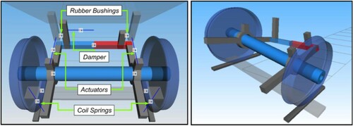
The anti-roll bar may be integrated in the frame taking advantage of the flexibility of the composite material used. The composite material frame is not designed in detail yet, a simple but effective representation of it is modelled in SIMPACK. To simulate the anti-roll bar, the required torsional stiffness of 250 kNm/rad without damping is introduced between two rigid halves of the frame. In this way, the necessary movement shown in Figure 1 (Right) can be achieved.

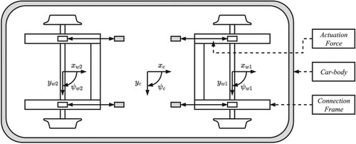
Longitudinal actuators are used to steer the wheelset into the desired position. They are considered ideal and able to produce the requested force without delay, which is a reasonable assumption for such slow control. A two-dimensional schematic representation of the innovative vehicle is given in Figure 2. Here, the local reference systems for the carbody and the two wheelsets are shown. Subscript c stands for carbody, 1 for leading wheelset and 2 for trailing wheelset; $y$ is the lateral displacement with respect to the track centre line and $\psi$ is the attack angle.

Figure 2. Top view of the innovative vehicle (Scheme).

The vehicle is supposed to run on Metro Madrid line 10 and a set of seven curves is selected to represent the line. Each simulation track case is composed by a tangent track with length 100 m, a linear transition curve of 100 m and a circular curve of 500 m. An exception is made for the narrowest considered curve (R = 100 m), in which the circular part has a reduced length of 300 m to avoid unrealistic overlapping between the beginning and the end of the curve. The exit transition curve is not used for the design of the feedforward controller, but it is included in Sub-section 6.2 for validation.

The maximum speed for each curve corresponds to a NLA of 0.65 m/s² while the minimum one is set to 10 km/h for all curves. In this way the behaviour of the vehicle can be simulated from a very low speed corresponding to a negative NLA (variable for each curve) to higher speeds with positive NLA (fixed for each curve), leading to a comprehensive study of the vehicle performance during curve negotiation. The largest considered curve (R = 1066 m) is generated from a track cant ($h$) of 60 mm and the admissible vehicle speed of 120 km/h with NLA equal to 0.65 m/s² (where the semi-wheel distance is $b_0=0.75$ m).

Seventeen speeds for each curve are generated starting from a NLA distribution. For each curve the speeds are given by a linear distribution of eight speeds between 10 km/h and the balanced speed (NLA = 0 m/s²), the balanced speed, and a linear distribution of eight speeds between the balanced speed and the speed corresponding to NLA equal to 0.65 m/s². In Figure 3 the speed distribution is shown in km/h for NLA against curve radius with the related track cant.

Figure 3. Speed distribution [km/h] as function of curve radius and NLA.

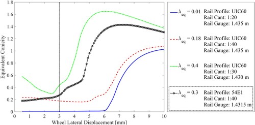
In order to evaluate the performance of the system on a wide range of operation conditions and develop a robust and effective feedforward control, three different equivalent conicities are considered during the control development phase: 0.01, 0.18 respectively 0.4. Different rail cants and track gauges are used while rail and wheel profiles are maintained constant as new UIC60 and S1002, respectively. In Sub-section 6.2, an additional equivalent conicity λ_eq= 0.3 is introduced to validate the capability of the feedforward approach to adapt to conicity variation. In this case, the rail profile 54E1 is used while the wheel profile is maintained as S1002. In Figure 4 the four equivalent conicity evolutions against wheel lateral displacement are shown.

Figure 4. Equivalent conicity as function of wheel lateral displacement.

3. Methodology

As stated, the aim of the paper is to find a suitable steering strategy to improve the curving performance of the proposed vehicle for all the previously defined running conditions. First, four families of feedback steering reference signals (approaches) are compared in terms of Tγ. The applied feedback approaches are selected from those found in the literature and designed for the current application. A cost function is created to evaluate the best reachable performance of the feedback approaches in terms of Tγ, applied actuation force and presence of a second contact point. The actuation forces required to obtain the best reachable performance are then used to generate the target force for the feedforward approach, which is validated through simulations with the defined running case scenarios. Tγ is again used to evaluate the effectiveness of the controller. Additionally, the feedforward approach is checked for a randomly selected conicity. The assumptions made during the described process are discussed in each respective section.

4. Feedback control

In this section the considered feedback approaches are described and applied, and their possible limitations are shown. The obtained simulation results are discussed, and stability issues are pointed out. The assumptions made at this stage are:

1. The tracks are considered ideal, i.e. without track irregularities.

2. Control signals are considered known without any uncertainty. Possible problems concerning the measurement of lateral displacement and attack angle of the wheelset are ignored.

3. Proportional–Integral–Derivative (PID) controllers are used to achieve zero steady-state error for all feedback approaches.

4. Robustness of the feedback controllers against curve, speed and conicity variation is not guaranteed. Every curve, speed and conicity combination may require a dedicated PID controller. In Sub-section 4.3, this issue is shortly discussed.

5. Only the circular part of the curve where zero steady state error is achieved by the feedback system is considered for the Tγ evaluation. Specifically, the last 40% of the circular curve is used.

6. Right-hand curves are considered with a positive sign while they are considered negative if they are left-hand curves.

7. Only right-hand curves are considered for the feedback phase.

4.1. Feedback approaches

Different reference signals can be considered for wheelset steering when applying feedback control. Among those, only the ones that are aiming to control the lateral wheelset position or the wheelset attack angle are studied in this paper. Thus, force feedback ([10]) is not considered. The possible reference signals can be divided into three main categories based on: geometric alignment, creep forces or NLA. Some of the approaches require simultaneous control of both lateral displacement and attack angle. Zero steady-state error cannot be achieved on both since lateral displacement and attack angle are not independent variables for a solid axle and the chosen actuator placements (Figure 2). Thus, when required, all possible combinations of lateral displacement and attack angle control are considered.

In total nine approaches divided in five groups are selected. Concerning the geometric alignment, Radial Steering (A) is considered. For creep-force based reference signals, Longitudinal and Lateral Creep Force Balance (B) and Tγ Minimisation (C) are introduced. NLA Compensation (D) is used for NLA based reference signals. Additionally, a combination of A and B concepts is introduced as Combined Approach (E).

1. Radial Steering control

A free wheelset aims at achieving an ideal position during curve negotiation which is a geometric alignment with the curve radius vector. In this case the attack angle is equal to zero. Thus, in Radial Steering control, the attack angle of each wheelset is commanded to be zero, (1) ${\psi }_{w1,2}^{ref}=0,$(1) where the superscript ref stands for reference signal.

(B)	Longitudinal and Lateral Creep Force Balance control

Taking Kalker’s linear theory for the relationship between creepages and creep forces ([23]) as starting point, it is possible to derive two conditions ([7]), (2) $\begin{array}{rl}& y_{w1,2}^{ref}=-b_0\frac{r_0}{{\lambda }_{eq}}\frac{1}{R},\end{array}$(2) (3) $\begin{array}{rl}& {\psi }_{w1}^{ref}-{\psi }_{w2}^{ref}=0,\end{array}$(3) where, $b_0$ is the semi-wheels distance and $r_0$ the nominal wheel radius. Equation (2) expresses which lateral position the wheelset should have to guarantee pure rolling condition. In this position, the longitudinal creep forces on each wheel ($F_{\xi }$) are balanced to produce zero moment on the wheelset itself, $b_0(F_{\xi }^L-F_{\xi }^R)=0$. Once Equation (2) is satisfied, the lateral creep forces ($F_{\eta }$) on the two wheelsets should be balanced with respect to each other, thus, $\sum F_{\eta }(w_1)-\sum F_{\eta }(w_2)=0$. Equation (3) expresses the requirement to achieve lateral creep force balance in terms of relative attack angle between the two wheelsets.

As stated before, it is not possible to reach zero steady-state error on both lateral displacement and attack angle simultaneously. Thus, two sub-cases are created:

• B₁: two PID controllers are used to achieve zero steady-state error for Equation (2) on both wheelsets,

• B₂: one PID controller is used to achieve zero steady-state error for Equation (3).

It should be noticed that the reference signals generated by Equation (2) may not be feasible. For instance, if conicity λ_eq= 0.01 is considered for the vehicle negotiating the 250 m curve with b₀= 0.75 m and r₀= 0.43 m, the reference lateral displacement will be −129 mm, which is clearly not feasible. Thus, the reference signal is limited to ± 5.8 mm for the equivalent conicities of 0.01 respectively 0.18 and ± 3.3 mm for equivalent conicity of 0.4 to avoid flange contact. The reduced reference range for equivalent conicity 0.4 is due to the reduced track gauge (Figure 4). In practice, for conicity 0.01, it is never possible to generate a feasible reference signal. For 0.18 and 0.4 conicities the reference signal generates feasible solutions for curve radius 400 m and larger and 250 m and larger, respectively. The reference signal limitation is due to the deficiency of the conical wheel linear theory in describing the shape of profiled wheels.

(C)	Tγ Minimisation control

Another possible approach based on longitudinal and lateral creep forces is based on the minimisation of the Tγ function ([23]), (4) $T\gamma =|F_{\xi }{\nu }_{\xi }|+|F_{\eta }{\nu }_{\eta }|+|M_{\zeta }\varphi |.$(4)

If the contribution of the spin is considered negligible compared to the other two, it is possible to derive the wheelset lateral position and attack angle that guarantee the minimum of the Tγ function, (5) $\begin{array}{rl}{y}_{w(n)}^{ref}& =-\frac{f_{11}({\lambda }_{eq}/r_0)(b_0/R)}{2f_{11}{({\lambda }_{eq}/r_0)}^2+(1/2)(f_{23}^2/f_{22})({\kappa }^2/r_0^2)},\end{array}$(5) (6) $\begin{array}{rl}{\psi }_{w(n)}^{ref}& =\frac{((1/2)(f_{23}/f_{22})(\kappa /r_0))(f_{11}({\lambda }_{eq}/r_0)(b_0/R))}{2f_{11}{({\lambda }_{eq}/r_0)}^2+(1/2)(f_{23}^2/f_{22})({\kappa }^2/r_0^2)}.\end{array}$(6)

Here, $\kappa =10$ m⁻¹ is the gravitational stiffness and $f_{11}=4$ MN, $f_{22}=3.3$ MN and $f_{23}=11$ kN/m are the considered Kalker coefficients ([24]). In Appendix 1 the derivation of the proposed minimum condition is provided. A similar derivation for a bogie vehicle was recently made by Tian et. al in [25].

The approach is introduced as an alternative to approach B, although it is difficult to implement due to the many parameters. The following sub-classes are defined:

• C₁: two PID controllers are used to achieve zero steady-state error for Equation (6) on both wheelsets,

• C₂: two PID controllers are used to achieve zero steady-state error for Equation (6) on the leading wheelset and Equation (5) on the trailing wheelset,

• C₃: two PID controllers are used to achieve zero steady-state error for Equation (5) on the leading wheelset and Equation (6) on the trailing wheelset,

• C₄: two PID controllers are used to achieve zero steady-state error for Equation (5) on both wheelsets.

As per approach B, it is not possible to fully apply Equation (5) for the lowest equivalent conicity. In this case, it is possible to apply the desired reference signal only on the 1066 m curve. Concerning the remaining conicities, the problem is less pronounced than in approach B. For equivalent conicities 0.18 and 0.4, the reference signal of Equation (5) must be limited only for the smallest curve (100 m).

(D)	NLA Compensation control

A different approach is represented by the possibility of controlling the attack angle of the wheelsets such that the centrifugal forces will be compensated ([8]). The desired attack angle for a two-axle vehicle is derived imposing that, on each wheelset, the lateral creep forces balance the centrifugal forces, $\sum F_{\eta }(w)=\sum m\text{NLA}$ ([12]). By expressing the relation between the lateral creep forces and the attack angle in quasi-static condition, it is possible to derive the reference signal (7) ${\psi }_{w(n)}^{ref}=\frac{m_w+(m_c/2)}{2f_{22}}\text{NLA}.$(7)

In the derivation of the reference signal, it is assumed that the carbody centrifugal force is equally distributed on both wheelsets. Here, the unsprung masses are summarised in $m_w$ consisting of the wheelset and the connecting frame masses.

(E)	Combined control

The combined feedback approach proposed here is derived from an initial investigation. It was observed that radial steering (approach A) generally produces positive effect concerning the front wheelset while approach B₁ improves the performance on the rear wheelset. Thus, a combination of the two is applied. To simplify approach B₁ and remove the dependency from the conicity, the lateral displacement is asked to be just proportional to the curvature. The two reference signals are (8) ${\psi }_{w1}^{ref}=0,y_{w2}^{ref}=-\beta \frac{1}{R},$(8) where, $\beta =0.58$ m². In this way, the feasibility problem of the reference signal is eliminated for all the running cases apart from the 100 m curve with 0.4 conicity, where it is again limited to ± 3.3 mm.

4.2. Results of feedback approaches

The feedback approaches are applied to the vehicle model developed in SIMPACK and described in Section 2. Here, it is important to remember the application of the assumptions made in the beginning of this section; in particular, assumption 4. This assumption will be discussed in Sub-section 4.3.

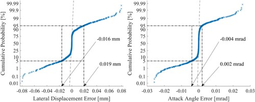
To ensure the relevance of the conclusions that will follow from the observation of the feedback approaches performance, it is useful to show a statistical evaluation of the average reference error from all the 3123 studied cases (357 running conditions and nine feedback approaches). In Figure 5 (Left) the cumulative probability distribution for the lateral displacement error is shown, disregarding to which feedback approach it belongs. In Figure 5 (Right) the same is done for the attack angle error. It can be seen that the lateral displacement error is in the interval ± 80 μm with 90% of the cases in the interval [−16, +19] μm. Concerning the attack angle, the errors are in the interval ± 26 μrad while 90% of the cases belongs to the interval [−4, +2] μrad. The achieved error distribution is sufficiently close to zero to assume that the results obtained from this analysis are reliable.

Figure 5. Reference tracking errors: Lateral Displacement (Left), attack angle (right). The vertical scale is made sectional logarithmic to highlight the tails (0–5% and 95–100%) of the distribution.

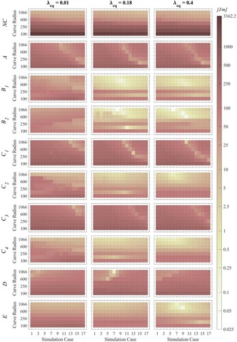
In Appendix 2, the performance in terms of Tγ function of each feedback approach together with the not controlled (NC) vehicle are shown as function of simulation case (NLA) and curve radius. In Figure A2.1 and Figure A2.2 the Tγ values are given for the leading respectively the trailing wheelset.

The results of Appendix 2 are summarised in Figure 6 per conicity and wheelset as the cumulative dissipated energy (CDE), which is derived by double integrating the Tγ values distributions first by the NLA and subsequently by the radius. Thus, it represents the volume underneath the Tγ distributions. Trapezoidal numerical integration has been used to achieve the results shown in Figure 6 since CDE is a comparison tool without accuracy requirements. The results are presented normalised to the maximum CDE per wheelset (achieved by the non-controlled vehicle). Thus, CDE values related to the leading wheelset are normalised with themselves and the same applies to the trailing wheelset.

Figure 6. Performance comparison between the feedback approaches in terms of normalised cumulative dissipated energy. The CDE values are expressed as percentage of the maximum achieved one per wheelset. Each bar groups the results for each feedback approach.

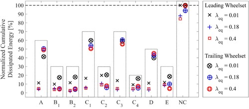
For all the cases, the application of a feedback approach reduces the CDE values. Only small differences can be observed for the leading wheelset among the different feedback approaches. In contrast, the trailing wheelset is significantly affected by the approach used. Characteristic of the cases where CDE shows a lower reduction is that the angle of attack is controlled to a predetermined position (A, C₁, C₃ and D). No extensive discussion about the reasons why this occurs will be made in this paper since the peculiarity of the vehicle structure may significantly influence the result. However, an explanation can be found in the dependency of the trailing wheelset from the leading one. According to [23], the Tγ function is significantly more affected by the lateral position of the wheelset than by the attack angle (Equation (A1)). Thus, commanding just the attack angle of the trailing wheelset does not ensure that the lateral position will be favourable. On the contrary, if the lateral position is controlled, even if the attack angle is not in a favourable position, its influence on the Tγ function will be less pronounced.

Lastly, it is important to underline that, according to the results shown in Figure 6 and Appendix 2 Figure A2.1 and A2.2, there is no best choice of feedback approach that covers all the running cases. This will be emphasised in Sub-section 5, where the actuation force is combined with the Tγ values in the cost function.

4.3. Discussion on stability issues

In this section the stability problems that can emerge in controlling the wheelset position of a railway vehicle are discussed. The discussion will indicate the complexity of the phenomena rather than being a deep investigation on possible methodologies to solve the mentioned problem.

As stated in Section 1, different methodologies can be applied to overcome the stability issues of feedback approaches. Among those, speed scaling (Schwarz et. al. [15] and Giossi et. al. [16]) can be an efficient and easy approach to implement. In this case the controller parameters vary depending on the speed. Enhancement of the feedback performance by having time varying parameters for the controller is also shown by Selamat et. al in [14] and recently by Tian et. al in [25].

As explicative example, the controlled vehicle running on the 400 m curve at 10 km/h (NLA = −0.63 m/s²) and 82 km/h (NLA = 0.65 m/s²) is considered. Here, the method proposed in [16] is used to guarantee stability and performance of the controlled vehicle with equivalent conicity 0.18 applying the feedback approach B₁ (Section 4.1.B). The equivalent conicity is then changed to 0.01 and 0.40 (Figure 4) without changing the controller. In Figure 7 it is possible to observe that the controller fails in producing reliable results when the conicity is changed and, in the example, for 10 km/h and conicity 0.40 it causes the vehicle to derail.

Figure 7. Leading wheelset lateral displacement with a controller designed for ${\lambda }_{eq}=0.18$ shown for different equivalent conicities against normalised time: speed equal to 10 km/h (Left) and speed equal to 82 km/h (Right).

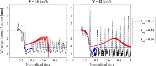
The example was chosen on purpose to show stability issues that may occur when conicity and speed are changed. Even if other feedback control approaches may be less sensitive, this example indicates the difficulties that must be overcome when applying a feedback control on a vehicle operating on varying conditions.

5. Cost function

A cost function is created to evaluate the performance of the feedback approaches, which will lead to the definition of the feedforward approach. The feedforward approach will aim at the best performance of the feedback approaches by estimating the actuation forces applied by the feedback approach with the largest benefit. The cost function combines the Tγ function values and the actuation forces used to achieve that Tγ value, simultaneously for the leading and the trailing wheelsets.

Each feedback approach may have positive or negative effect on the vehicle performance according to the running condition. It can have a positive effect on the leading wheelset but negative effect on the trailing one and vice versa. Moreover, two approaches may result in similar values of the Tγ function, but one of the two requires less actuation force than the other. Concentrating only on the Tγ value can cause excessive force requirement while, in contrast, concentrating only on one of the two wheelsets can cause unacceptable performance on the other one.

In order to select which feedback approach is ‘optimal’ for a certain running case, the cost function: (9) $C=\frac{1}{{\alpha }_1}(T_{\gamma ,1}+T_{\gamma ,2})+\frac{1}{{\alpha }_2}(|F_1|+|F_2|)+\frac{1}{{\alpha }_3}(T_{\gamma ,1,L}^{2^{nd}}+T_{\gamma ,1,R}^{2^{nd}}+T_{\gamma ,2,L}^{2^{nd}}+T_{\gamma ,2,R}^{2^{nd}}),$(9) is created for each running case (curve, NLA and conicity) and feedback approach. The global Tγ value per wheelset ($T_{\gamma ,1}$ and $T_{\gamma ,2}$), the requested actuation force per wheelset ($|F_1|$ and $|F_2|$) and the second contact point Tγ value per each wheel ($T_{\gamma ,1,L}^{2^{nd}}$, $T_{\gamma ,1,R}^{2^{nd}}$, $T_{\gamma ,2,L}^{2^{nd}}$ and $T_{\gamma ,2,R}^{2^{nd}}$) are considered at the same time. In this way, a feedback approach that has low Tγ values and actuation force requirement on both wheelsets simultaneously without presence of a second contact point has a low value of the cost function. Searching the minimum of the cost function means that for a specific running case the feedback approach related to that case has the lowest combination of Tγ values, actuation forces and presence of second contact point.

A normalisation between different quantities is done. In Equation (9), ${\alpha }_1=300$ J/m, ${\alpha }_2=90$ kN and ${\alpha }_3=50$ J/m are chosen. In this way, an average value of the Tγ function of 150 J/m is considered acceptable for each wheelset, 45 kN are acceptable for the actuation force and 12.5 J/m are acceptable for each second contact point. With this approach, the presence of a second contact point is heavily penalised. The Tγ ${\alpha }_1$ value is chosen as maximum value to avoid severe wear while the force value is chosen to foresee a reasonable actuator force considering a suitable dimension of it. According to a recent study (RUN2Rail [26]) electromechanical actuators can be a suitable choice for the active steering purpose. Regarding the second point contact, the acceptable value is tuned in accordance with the results of the cost function. It was observed that when the second contact point factor ${\alpha }_3$ was set to be one sixth of ${\alpha }_1$ the cost function was able to select controllers that produce negligible second contact point wear. The normalisation procedure significantly influence the results of the cost function and it can be tuned differently for specific purposes.

The required actuation forces corresponding to the minimum of the cost function are stored for each running case and for each wheelset independently. Thus, for each conicity case, a distribution of desired forces is achieved as function of NLA and curve radius. The feedforward approach is then generated starting from the obtained force distributions.

5.1. Cost function results

The results of the feedback approaches are analysed with the cost function introduced above. For each running condition, the cost function of Equation (9) is calculated per feedback approach. The obtained results are compared among the considered feedback approaches and for each running condition the lowest value of the cost function is chosen.

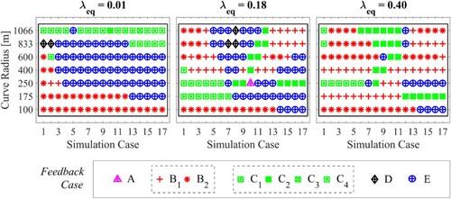
Since the cost function takes into consideration both wheelsets at the same time, looking at Figure 6, it can be foreseen that the feedback approaches A, C₁, C₃ and D are less likely to be chosen. Among the remaining ones, the decision will be largely related to the required actuation force and the presence of a second contact point. Generally, the B feedback approaches show low presence of a second contact point but, at the same time, they require the highest actuation force. A similar behaviour is shown by approaches C while approach E shows among the smallest actuation force. In Figure 8 the achieved decision table is shown. For each running condition, the feedback approach that gives the minimum of the cost function in that condition is displayed. In the overall 357 running cases, approach A has been chosen 1 time, approach B, 160 times (B₁ 64 and B₂ 96 times), approach C, 77 times (C₁, C₂, C₃ and C₄ 0, 34, 1 respectively 42 times), approach D, 5 times and approach E, 114 times. For the studied vehicle, it can be concluded that, if a feedback approach is meant to be implemented, it is less beneficial or in some cases disadvantageous (Appendix 2) to control the trailing wheelset to a pre-specified attack angle than let it be uncontrolled. Controlling its lateral position (approaches B₁, C₂, C₄, E) or applying the same attack angle as the leading wheelset (B₂) gives better results.

Figure 8. Decision table for selecting the feedback approach giving the lowest cost for equivalent conicity 0.01 (Left), 0.18 (Centre) and 0.40 (Right).

6. Feedforward control

This section presents the development of the feedforward control and results obtained by its application to the defined running cases. As in Section 4, it is important to underline the assumptions made:

1. Each simulation track case is considered ideal. Track irregularities are introduced in a later stage to validate the controller.

2. Right-hand curves are considered with a positive sign while they are considered negative if they are left-hand curves.

3. Only right-hand curves are considered during the development of the feedforward approach.

6.1. Feedforward control generation

Different methods can be used to manage the force distributions determined by the cost function introduced in Section 5. Among them, a least square approximation is chosen as it is easy to implement and generates robust results with sufficient approximation precision. Moreover, it can help in reducing the number of variables that must be considered at the approximation.

In this paper, it is chosen to approximate the force distribution as a function of NLA and curvature. For each wheelset (10) $F=(a_1\text{NLA}+a_2{)}^n{\left(b_1\frac{1}{R}+b_2\right)}^m,$(10) where, $n$ and $m$ can take the values 1 (linear dependence) and 2 (squared dependence) creating four possible polynomial approximation functions, (11) $\begin{array}{rl}{F}_{n=2,m=2}& =k_1\text{NL}{\text{A}}^2{\left(\frac{1}{R}\right)}^2+k_2\text{NLA}{\left(\frac{1}{R}\right)}^2+k_3{\left(\frac{1}{R}\right)}^2+k_4\text{NL}{\text{A}}^2\left(\frac{1}{R}\right)\\ & +k_5\text{NLA}\left(\frac{1}{R}\right)+k_6\left(\frac{1}{R}\right)+k_7\text{NL}{\text{A}}^2+k_8\text{NLA}+k_9,\\ F_{n=1,m=2}& =k_2\text{NLA}{\left(\frac{1}{R}\right)}^2+k_3{\left(\frac{1}{R}\right)}^2+k_5\text{NLA}\left(\frac{1}{R}\right)+k_6\left(\frac{1}{R}\right)+k_8\text{NLA}+k_9,\\ F_{n=2,m=1}& =k_4\text{NL}{\text{A}}^2\left(\frac{1}{R}\right)+k_5\text{NLA}\left(\frac{1}{R}\right)+k_6\left(\frac{1}{R}\right)+k_7\text{NL}{\text{A}}^2+k_8\text{NLA}+k_9,\\ F_{n=1,m=1}& =k_5\text{NLA}\left(\frac{1}{R}\right)+k_6\left(\frac{1}{R}\right)+k_{8}NLA+k_9.\end{array}$(11)

NLA and curvature are chosen for two main reasons, the first being that NLA and curvature are key parameters that describe the vehicle's driving conditions, the other is that they can be estimated with inexpensive sensors. This has been used in tilting trains ([21]), where the NLA is estimated by an accelerometer in the running gear and the curvature by a rate gyroscope in the carbody centre ${\dot{\psi }}_c$ combined with a tachometer that gives the vehicle speed$v$, (12) $\frac{1}{R}=\frac{{\dot{\psi }}_c}{v}.$(12)

To create a feedforward controller that is applicable to any operational case, the least square approximation method is applied to the average required force between the three conicities.

Due to the second and third assumptions in Section 6, the symmetry of the generated feedforward controller with respect to the curvature is not guaranteed. Thus, the final controller is symmetrised with respect to the sign of the curvature to give the desired effect when negotiating left-hand curves.

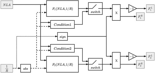
The approximation was found to generate inversed actuation forces for large curve radii. For this reason, for each combination of Equation (10) and for each wheelset it is required that $F(\text{NLA},1/R)\ge 0$. The solution is easily determined as a condition on the curvature if NLA is treated as a known variable parameter. At the same time, the performance of the vehicle for curve radii above 2000 m are sufficiently good to not require any action. Thus, for each wheelset a condition is introduced to avoid the control action if inversion of the actuation force and/or a curve radius above 2000 m are detected. In Figure 9 the feedforward control scheme is shown.

Figure 9. Feedforward control scheme.

The simplicity of the approach may introduce significant deviations from the desired force distribution obtained through the minimum of the cost function. If a more complex approximation is to be applied (such as interpolation methods or lookup tables), additional information may be required, for example conicity. Estimation of conicity is a complicated process, which preferably should be performed in real time on the train to handle the local conditions ([27]).

6.2. Results on feedforward approaches

The force distribution determined by the cost function is here approximated by the expressions given in Equation (11) and tested on the defined running cases for the vehicle described in Section 2. Lastly, to prove the applicability of the proposed approach against a variety of conditions a new running case with track irregularities is introduced.

For each wheelset, the least square approximation is applied to determine the coefficients of the four considered approximation functions. In Table 2 the coefficients are provided for both leading and trailing wheelsets.

Table 2. Approximation functions coefficients. Each column gives the possible combinations of the exponents of Equation (10). Each row gives the coefficients that must be multiplied by the variables (NLA and 1/R) as shown in Equation (11).

	Leading wheelset				Trailing wheelset
	n=1, m=1	n=2, m=1	n=1, m=2	n=2, m=2	n=1, m=1	n=2, m=1	n=1, m=2	n=2, m=2
$k_1$	∖	∖	∖	8.99e8	∖	∖	∖	1.10e9
$k_2$	∖	∖	9.62e8	9.87e8	∖	∖	5.74e8	6.82e8
$k_3$	∖	∖	8.82e7	−5.28e7	∖	∖	6.16e8	4.21e8
$k_4$	∖	8.22e5	∖	−9.97e6	∖	−5.30e6	∖	−1.56e7
$k_5$	2.22e6	2.03e6	−7.79e6	−8.11e6	−2.75e6	−1.55e6	−9.00e6	−9.42e6
$k_6$	1.43e7	1.42e7	1.33e7	1.49e7	1.51e7	1.56e7	8.51e6	1.10e7
$k_7$	∖	−2.17e3	∖	1.47e4	∖	1.17e4	∖	3.05e4
$k_8$	−1.85e4	−1.78e4	−1.39e3	−1.83e3	−4.49e3	−8.78e3	5.33e3	3.41e3
$k_9$	3.60e3	3.76e3	4.98e3	2.88e3	−1.14e4	−1.21e4	−1.03e3	−5.19e3

The approximation functions are not symmetric with respect to the curvature, thus, the symmetrisation procedure introduced in Sub-section 6.1 is applied to avoid undesired behaviour in left-hand curves.

To evaluate which of the approximation functions is the best choice, they are applied to all the running cases previously defined. Additionally, their efficiency is tested against a new wheel-rail combination not used when deriving the feedforward approach. The new equivalent conicity of 0.3 is achieved by using the S1002 wheel profile as previously, but changing the rail profile to the 54E1, the track gauge to 1.4315 m and imposing a rail cant of 1:40 (Figure 4). The CDE is shown in Figure 10, normalised with respect to the not controlled vehicle. Here again, the normalisation is done independently for the leading and trailing wheelset.

Figure 10. Performance comparison between the feedforward approaches in terms of normalised cumulative dissipated energy. Each bar groups the results for each feedforward approximation function.

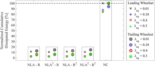
All feedforward approximations produce similar results and improve the performance compared to the not controlled vehicle in terms of CDE. Since no significant difference is observed among the four approximations, the simplest one is chosen (n=1, m=1 in Equation (10)). In Figure 11 the average Tγ values for each running case (taken accordingly to assumption five in Section 4) are shown for the four considered conicities. The results achieved with the chosen feedforward approach (FF) are compared with the ones of the not controlled vehicle (NC). It is possible to see that a significant reduction of the Tγ value is achieved for all the simulations. This is especially evident for the high conicities and small curve radii. Concerning the trailing wheelset, the improvements are less significant in large curve radii with respect to the leading wheelset. However, for curve radii above 400 m, the maximum obtained Tγ value is approximately 50 J/m.

Figure 11. Tγ distribution for the not controlled vehicle (NC) and the feedforward controlled (FF). Leading wheelset (Top) and trailing wheelset (Bottom).

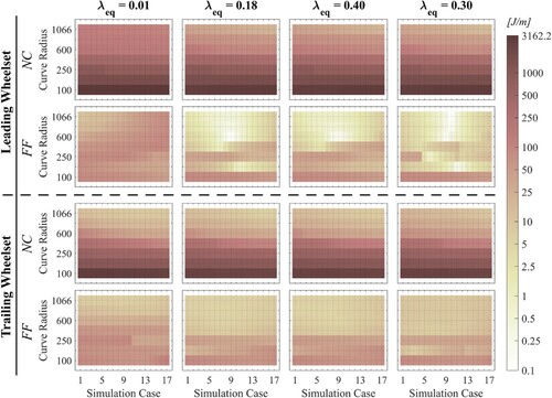
To produce the results in Figure 11, a maximum actuation force of about 150 kN is used in the 100 m curve for NLA equal to 0.65 m/s² for the leading wheelset and a maximum force of 170 kN is used for NLA equal to −0.32 m/s² for the trailing wheelset. Such high forces can cause a derailment risk in case of malfunctioning motivating a force limitation on the expense of less good performance in very tight curves.

Finally, an example of how the control behaves when negotiating two curves with and without track irregularities is presented in Figure 12. The results are shown in terms of Tγ against normalised time. One of the original running cases is firstly chosen (Figure 12 (Top)) where the vehicle with 0.18 equivalent conicity is running into the 175 m curve at a speed of 54 km/h (NLA = 0.65 m/s²). Additionally, the performance of the control against curve variation is addressed (Figure 12 (Bottom)). A randomly generated curve is created with curve radius of 711 m and cant of 130 mm. The vehicle is running at a speed of 94 km/h (NLA = 0.11 m/s²) chosen randomly between 10 and 117 km/h (NLA = 0.65 m/s²). The chosen conicity for this last test case is 0.3, i.e. the fourth one introduced. Both tracks are composed by 100 m of tangent track, 100 m of transition curve, 500 m of circular curve, 100 m of transition curve and finally 100 m of tangent track. Additionally, track irregularities ERRI_High [28] are introduced. The simulations results show that the feedforward control provides satisfying solutions for both leading and trailing wheelset even when track irregularities are introduced.

Figure 12. Time simulation results on two different running cases comparing the controlled and not controlled vehicle: equivalent conicity 0.18, curve radius 175 m, speed 54 km/h (Top), equivalent conicity 0.3, curve radius 711 m, speed 94 km/h (Bottom), leading wheelset (Left) and trailing wheelset (Right).

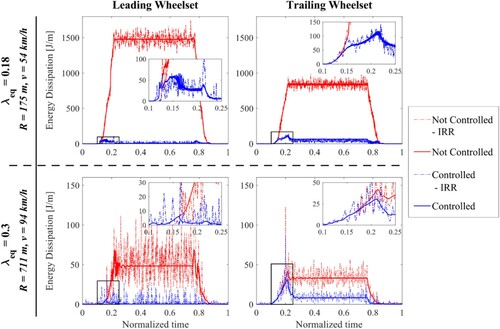
A control delay appears in the entry transition curve for the trailing wheelset, which reduces the performance of the proposed feedforward approach in short curve transitions. An explanation can be found in the forces that the carbody imposes on the wheelsets. For the trailing wheelset those forces are ahead of the wheelset itself. This is particularly evident where there is no quasi-static equilibrium, i.e. in the transition curve. The problem can be overcome with a feedforward approach dedicated to solve the delay problem in transition curve as proposed in [15,29] or by using signals coming from the preceding vehicles as done in tilting trains ([21]). Nevertheless, in the circular part of the curve, a reduction of approximately 92% for the 175 m curve 75% for the 711 m curve in terms of Tγ function for the trailing wheelset is achieved while a reduction of 99% for the 175 m curve and 97% for the 711 m curve is observed for the leading wheelset.

7. Conclusions and future work

The paper presents a procedure to develop a feedforward control approach for wheelset steering for an innovative two-axle vehicle that avoids the standard feedback sensing problems using easily available measurement signals such as NLA and carbody yaw velocity. The approach is based on control forces applied by the feedback control with the best performance of several studied approaches in 7 possible curves, 17 speeds per curve and 3 conicities.

From the studied feedback approaches, it can be seen that no perfect solution exists among the studied feedback approaches when Tγ, required actuation force and the presence of the second contact point are considered, i.e. the best performance is achieved by different feedback approaches in different operation cases.

The feedforward approach reduces Tγ with 92% for the leading and 75% for the trailing wheelset compared to the passive vehicle as an average for studied running cases. It is shown that the performance is not significantly influenced by conicity, curvature, speed, or presence of track irregularities.

The feedforward approach tends to require larger actuator forces than practically reasonable in the narrowest curves and a too late response for the trailing wheelset in curve entry transitions.

We believe that the presented approach is applicable not only to the single axle vehicle introduced here, but to all types of rail vehicles. The advantages compared to traditional feedback approaches are a simpler controller using easier measured properties and less sensitivity to track variations.

In future studies the influence of frame flexibility should be investigated by replacing the rigid halved model of the connection frame by a finite element model. Actuator models should be implemented to validate the assumption of ideal actuators made in section 2. The influence of force saturation due to possible actuator size should be investigated together with possibilities to reduce the delay in curve entry transitions for the trailing wheelset. Finally, the performance of the defined vehicle with the proposed controller should be addressed for a full operational scenario at realistic running conditions.

Acknowledgments

This project has received funding from the Shift2Rail Joint Undertaking under the European Union’s Horizon 2020 research and innovation programme under grant agreement (No. 777564). The content of this paper reflects only the author's view and the JU is not responsible for any use that may be made of the information it contains.

Disclosure statement

No potential conflict of interest was reported by the author(s).

Additional information

Funding

This project has received funding from the Shift2Rail Joint Undertaking under the European Union’s Horizon 2020 research and innovation programme under grant agreement (No. 777564). The content of this paper reflects only the author's view and the JU is not responsible for any use that may be made of the information it contains.

Appendices

Appendix 1

The derivation of Equations (5) and (6) is done by means of some assumptions. Firstly, Kalker’s linear theory is considered to be applicable. Secondly, the spin contribution in Equation (4) is considered negligible. Moreover, considering the vehicle negotiating the circular part of the curve, only the quasi-static contributions are taken into account, thus, the derivatives with respect to time are neglected. Following these assumptions, the Tγ function ([23]) can be written as: (A1) $T_{\gamma }=f_{11}\left|{\left(\frac{{\lambda }_{eq}}{r_0}\right)}^2{y}_w^2+\frac{{\lambda }_{eq}}{r_0}\frac{b_0}{R}{y}_w+{\left(\frac{b_0}{R}\right)}^2\right|+\left|f_{22}{\psi }_w^2+f_{23}\frac{\kappa }{r_0}{y}_w{\psi }_w\right|,$(A1) or equivalently as: $T_{\gamma }=f_{11}|g(y_w)|+|h(y_w,{\psi }_w)|$. It can be shown that Tγ is a strictly positive function. Even if $h(y_w,{\psi }_w)=0$ for ${\psi }_w=0$, $g(y_w)$ is a strictly positive quadratic function in $y_w$ since $({\lambda }_{eq}/r_0{)}^2>0$ and (A2) $y_{w1,2}=\frac{1}{2}\frac{b_0}{R}\frac{r_0}{{\lambda }_{eq}}\left(-1\pm j\sqrt{3}\right),$(A2) are solutions of $g(y_w)=0$.

To derive the minimum of the Tγ function, it is necessary to find the conditions for which the gradient is equal to zero: (A3) $\mathrm{\nabla }{T}_{\gamma }=\left[\frac{\mathrm{\partial }{T}_{\gamma }}{\mathrm{\partial }{y}_w};\frac{\mathrm{\partial }{T}_{\gamma }}{\mathrm{\partial }{\psi }_w}\right]=0.$(A3)

It is useful to start form the derivative with respect to the attack angle. In this way it is possible to establish a direct relation between the attack angle and the lateral displacement. (A4) $\begin{array}{rl}\frac{\mathrm{\partial }{T}_{\gamma }}{\mathrm{\partial }{\psi }_w}& =\frac{|h(y_w,{\psi }_w)|}{h(y_w,{\psi }_w)}\cdot \frac{\mathrm{\partial }h(y_w,{\psi }_w)}{\mathrm{\partial }{\psi }_w}=\frac{|h(y_w,{\psi }_w)|}{h(y_w,{\psi }_w)}\left(2f_{22}{\psi }_w+f_{23}\frac{\kappa }{r_0}{y}_w\right)\\ & =sign\left(\frac{|h(y_w,{\psi }_w)|}{h(y_w,{\psi }_w)}\right)\left(2f_{22}{\psi }_w+f_{23}\frac{\kappa }{r_0}{y}_w\right)=0\end{array}$(A4)

Since, $sign(|h(y_w,{\psi }_w)|/h(y_w,{\psi }_w))$ does not affect the solution, the relation (A5) ${\psi }_w=-\frac{1}{2}\frac{f_{23}}{f_{22}}\frac{\kappa }{r_0}{y}_w,$(A5) can be achieved. The derivative with respect to the lateral displacement can now be considered. (A6) $\begin{array}{rl}\frac{\mathrm{\partial }{T}_{\gamma }}{\mathrm{\partial }{y}_w}& =f_{11}\frac{|g(y_w)|}{g(y_w)}\cdot \frac{\mathrm{\partial }g(y_w)}{\mathrm{\partial }{y}_w}+\frac{|h(y_w,{\psi }_w)|}{h(y_w,{\psi }_w)}\cdot \frac{\mathrm{\partial }h(y_w,{\psi }_w)}{\mathrm{\partial }{y}_w}\\ & =f_{11}\frac{|g(y_w)|}{g(y_w)}\cdot \left(2{\left(\frac{{\lambda }_{eq}}{r_0}\right)}^2{y}_w+\frac{{\lambda }_{eq}}{r_0}\frac{b_0}{R}\right)+\frac{|h(y_w,{\psi }_w)|}{h(y_w,{\psi }_w)}\cdot f_{23}\frac{\kappa }{r_0}{\psi }_w=0.\end{array}$(A6)

Since, $g(y_w)$ is a strictly positive function, $|g(y_w)|/g(y_w)=1$. Concerning $|h(y_w,{\psi }_w)|/h(y_w,{\psi }_w)$, the condition $y_w\ne 0$ must be satisfied. This condition is consistent as long as the vehicle is negotiating a curve. Substituting the solution of Equation (A5): (A7) $\begin{array}{rl}\frac{|h(y_w,{\psi }_w)|}{h(y_w,{\psi }_w)}& =sign\left(\frac{|h(y_w,{\psi }_w)|}{h(y_w,{\psi }_w)}\right)=sign(h(y_w,{\psi }_w))\\ & =sign\left(f_{22}{({\psi }_w)}^2+f_{23}\frac{\kappa }{r_0}{y}_w{\psi }_w\right)=sign\left(\frac{1}{4}\frac{f_{23}^2}{f_{22}}\frac{{\kappa }^2}{{r_0}^2}{(y_w)}^2-\frac{1}{2}\frac{f_{23}^2}{f_{22}}\frac{{\kappa }^2}{{r_0}^2}{(y_w)}^2\right)\\ & =\text{s}ign\left(-\frac{1}{4}\frac{f_{23}^2}{f_{22}}\frac{{\kappa }^2}{{r_0}^2}{(y_w)}^2\right)=-1.\end{array}$(A7)

Substituting Equations (A5) and (A7) into Equation (A6) it is possible to write Equation (A6) as only function of $y_w$, (A8) $\frac{\mathrm{\partial }{T}_{\gamma }}{\mathrm{\partial }{y}_w}=2f_{11}{\left(\frac{{\lambda }_{eq}}{r_0}\right)}^2{y}_w+f_{11}\frac{{\lambda }_{eq}}{r_0}\frac{b_0}{R}+\frac{1}{2}\frac{f_{23}^2}{f_{22}}\frac{{\kappa }^2}{{r_0}^2}{y}_w=0.$(A8)

The solution to Equation (A8) gives the reference signal of Equation (5). When Equation (5) is substituted into Equation (A5) the reference signal of Equation (6) can be obtained.

Since Tγ is a strictly positive function and only one solution of $\mathrm{\nabla }{T}_{\gamma }=0$ exists, the couple represented by Equations (5) and (6) is the minimum of the Tγ function as function of $y_w$ and ${\psi }_w$.

Appendix 2

Figure A1. Tγ distribution for feedback approaches: leading wheelset.

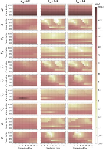
Figure A2. Tγ distribution for feedback approaches: trailing wheelset.

References

- Fu B, Giossi RL, Persson R, et al. Active suspension in railway vehicles: a literature survey. Railw. Eng. Sci. Mar. 2020;28:3–35. https://doi.org/https://doi.org/10.1007/s40534-020-00207-w
- Bruni S, Goodall R, Mei TX, et al. Control and monitoring for railway vehicle dynamics. Veh Syst Dyn Jul. 2007;45(7–8):743–779. doi: https://doi.org/10.1080/00423110701426690
- Polach O. Curving and stability optimisation of locomotive bogies using interconnected wheelsets. Veh Syst Dyn 2004;41(SUPPL):53–62.
- Park J-H, Koh H-I, Hur H-M, et al. Design and analysis of an active steering bogie for urban trains. J Mech Sci Technol 2010;24(6):1353–1362. doi: https://doi.org/10.1007/s12206-010-0341-4
- Umehara Y, Kamoshita S, Ishiguri K, et al. Development of electro-hydraulic actuator with fail-safe function for steering system. Q Rep RTRI. 2014;55(3):131–137. doi: https://doi.org/10.2219/rtriqr.55.131
- Shen G, Goodall R. Active yaw relaxation for improved bogie performance. Veh Syst Dyn 1997;28:273–289. doi: https://doi.org/10.1080/00423119708969357
- Pérez J, Busturia JM, Goodall RM. Control strategies for active steering of bogie-based railway vehicles. Control Eng Pract 2002;10(9):1005–1012. doi: https://doi.org/10.1016/S0967-0661(02)00070-9
- Shen S, Mei TX, Goodall RM, et al. A study of active steering strategies for railway bogie. Veh Syst Dyn 2004;41(suppl):282–291.
- Shen S, Mei TX, Goodall RM, et al. Active steering of railway vehicles: a feedforward strategy. In: 2003 European Control Conference (ECC), Cambridge, UK; 2003. p. 2390–2395.
- Shen S, Mei TX, Goodall RM, et al. A Novel control strategy for active steering of railway bogies. Proceedings of the Control 2004 Conference. 2004;September. http://ukacc.group.shef.ac.uk/proceedings/control2004/Papers/085.pdf
- Braghin F, Bruni S, Resta F. Active yaw damper for the improvement of railway vehicle stability and curving performances: simulations and experimental results. Veh Syst Dyn 2006;44(11):857–869. doi: https://doi.org/10.1080/00423110600733972
- Qazizadeh A, Stichel S, Feyzmahdavian HR. Wheelset curving guidance using H∞control. Veh Syst Dyn 2018;56(3):461–484. doi: https://doi.org/10.1080/00423114.2017.1391396
- Skogestad S., Postlethwaite I. Multivariable feedback control - analysis and design. 3rd ed. Chichester: WileyBlackwell; 2001.
- Selamat H, Yusof R, Goodall RM. Self-tuning control for active steering of a railway vehicle with solid-axle wheelsets. IET Control Theory Appl 2008;2(5):374–383. doi: https://doi.org/10.1049/iet-cta:20070111
- Schwarz C, Keck A, Brembeck J, et al. Control development for the scaled experimental railway running gear of DLR. 24th Symposium of the International Association for Vehicle System Dynamics (IAVSD 2015). 2016;1:909–918.
- Giossi RL, Persson R, Stichel S. Gain scaling for active wheelset steering on innovative two-axle vehicle. In Advances in dynamics of vehicles on roads and tracks. IAVSD 2019; 2020. p. 57–66.
- Mousavi Bideleh SM, Mei TX, Berbyuk V. Robust control and actuator dynamics compensation for railway vehicles. Veh Syst Dyn 2016;54(12):1762–1784. doi: https://doi.org/10.1080/00423114.2016.1234627
- Farhat N, Ward CP, Goodall RM, et al. The benefits of mechatronically-guided railway vehicles: a multi-body physics simulation study. Mechatronics (Oxf). 2018;51(March):115–126. doi: https://doi.org/10.1016/j.mechatronics.2018.03.008
- Mei TX, Goodall RM, Li H. Kalman filter for the state estimation of a 2-axle railway vehicle..
- Heckmann A, Schwarz C, Keck A, et al. Nonlinear observer design for guidance and traction of railway vehicles. In: Advances in dynamics of vehicles on roads and tracks. IAVSD 2019; 2020. p. 639–648.
- Persson R, Goodall RM, Sasaki K. Carbody tilting – technologies and benefits. Veh Syst Dyn Aug. 2009;47(8):949–981. doi: https://doi.org/10.1080/00423110903082234
- Hwang IK, Hur HM, Kim MJ, et al. Analysis of the active control of steering bogies for the dynamic characteristics on real track conditions. Proc. Inst. Mech. Eng. Part F J. Rail Rapid Transit. 2018;232(3):722–733. doi: https://doi.org/10.1177/0954409716687454
- Andersson E, Berg M, Stichel S. Rail vehicle dynamics; 2014.
- Kalker JJ. Review of wheel/rail rolling contact theories, the general problem of rolling contact. Appl. Mech. Div. ASME. 1980;40:72–92.
- Tian S, Luo X, Ren L, et al. Active steering control strategy for rail vehicle based on minimum wear number. Veh Syst Dyn Mar. 2020: 1–26. https://www.tandfonline.com/doi/full/https://doi.org/10.1080/00423114.2020.1743864
- Goodall R, Persson R, Baeza L, et al. Innovative Running Gear Solutions for New Dependable, Sustainable, Intelligent and Comfortable Rail Vehicles: Deliverable 3.1; 2019.
- Charles G, Goodall R, Dixon R. Model-based condition monitoring at the wheel-rail interface. Veh Syst Dyn 2008;46(SUPPL.1):415–430. doi: https://doi.org/10.1080/00423110801979259
- Bergander B, Kunnes W. ERRI B176/DT 290: B176/3 benchmark problem, results and assessment. Tech. report, Eur. Rail Res. Inst.; 1993.
- Grether G. Dynamics of a running gear with IRWs on curved tracks for a robust control development. Pamm. 2017;17(1):797–798. doi: https://doi.org/10.1002/pamm.201710366