Detailed wheel/rail geometry processing using the planar contact approach

Abstract

The use of detailed wheel/rail contact models has long been frustrated by the complicated preparations needed, to analyse the profiles for the local geometry and creep situation for the planar contact approach. A new software module is presented for this that automates the calculations in a generic way. Building on many components developed by others, this greatly simplifies the running of CONTACT for generic wheel/rail contact situations. Fully 3-d contact search algorithms are implemented. This uses the contact locus approach, that's simplified for wheel-on-rail situations and extended to wheel-on-roller contacts. A main characteristic of the new module is its extensive use of the multibody formalism, using markers to represent coordinate systems, using a newly designed, generic, object oriented-like software foundation. The contact geometry is analysed twice; first for the location of contact patches, and then for the local geometry of the contact patches. The contact search starts from profiles in their actual, overlapping positions. This yields the extent of interpenetration areas as needed for the potential contact definition. Different strategies may be employed for the tangent plane needed in the planar contact method. Creepages are formed automatically using rigid body kinematics, including wheel and track flexible bending. Numerical results illustrate the viability, generality, and robustness of the approach. The extension to conformal contacts is presented in an accompanying paper.

Keywords:

• Wheel-rail contact
• wheel-rail profile
• contact geometry
• contact forces
• planar contact
• software design

1. Introduction

Wheel/rail contact plays an essential role in rail vehicle systems, carrying the vehicle load, guiding the vehicle along the track curve, and allowing for traction and braking. Large loads are carried on small contact patches, such that high stresses arise, with consequent challenges for the material and geometrical design. As such, wheel/rail contact is a topic of continued research, from the perspectives of rail vehicle dynamics [1–3], and wear and rolling contact fatigue [4,5].

The CONTACT model is currently considered as ‘the golden standard’ for wheel/rail contact evaluation [6,7]. It was developed in the 1970-ies and 80-ies by professor Kalker [8–12]. The model is used at many places where detailed contact investigations are wanted, e.g. [13], and several researchers programmed their own version of Kalker's equations, e.g. [14–18]. The original software was acquired by VORtech BV in the year 2000, at Kalker's retirement from Delft University of Technology. VORtech extended the programme with respect to the speed of computations [19–21] and the physics involved, including the effects of interfacial layers [22–24] and conformal contact situations [25,26]. Free and commercial versions have been provided since 2009 with annual updates. The software was recently transferred to the company Vtech CMCC that now continues this development and distribution [27].

The use of the CONTACT software has long been complicated, due to a variety of compounding factors. A first one is the complexity of rolling contact mechanics itself, using concepts such as penetration and creepage that may be difficult to understand and relate to one's main object of study, and because of a lot of mathematics is involved in the solution. A second reason comes from the focus of the original CONTACT software, concentrating on the contact mechanics side of the problem, rather than the embedding in the context of vehicle system dynamics. This placed the burden on the user to define a suited local coordinate system and perform the corresponding preparations, providing the undeformed distance and rigid slip functions as inputs to CONTACT. This restricted the possible application of the CONTACT software.

Many works have been published on the incorporation of wheel/rail contact in vehicle dynamics, e.g. [28–31], and on the subsequent contact geometry problem [32–41]. However, these works don't deliver completely workable solutions as needed by CONTACT. Besides the location of contact patches, this further needs suitable choices for the tangent plane and coordinate origin [42], estimates for the extent of the contact patches [33], a suitable grid definition, and the calculation of the undeformed distance function. No general solution has been published to date for the automated running of CONTACT for generic wheel/rail contact situations. As a result, researchers may put CONTACT aside as being too complicated, or waste time on the re-development of profile smoothing and interpolation by themselves, or settle for short-cuts, ignoring the effects of the yaw angle, for instance, that may reduce confidence in the results.

This paper presents the software module for automated wheel/rail geometry processing that has been implemented in CONTACT. This greatly simplifies the use of CONTACT for wheel/rail contact investigation. Its design provides for detailed analyses in a generic way, allows for batch operation, and for the on-line integration in vehicle dynamics simulation. The techniques that are used mostly build upon the works of others before us: the cited references [32,34–36,40], the multibody formalism as presented by Shabana [43], and our fruitful interactions with SIMPACK, RecurDyn, and other providers of vehicle dynamics software. The main contribution lies in the combination of these ideas, on the basis of an extended vocabulary for working with markers, coordinates, and coordinate transformations, and the corresponding software foundation. A further novelty concerns the contact locus approach, that is simplified for wheel-on-track situations and extended to wheel-on-roller configurations. A final benefit of the approach that is presented lies in its extension to conformal contact situations. This is addressed in a separate paper [44].

This paper is structured as follows. Section 2 describes the software foundation, introducing the main concepts for coordinates and coordinate transformations. Section 3 gives an overview of software design issues and the approach followed for contact geometry processing, and elaborates on the main steps that are used. The extension of the contact locus approach is presented in Section 4. After this, Section 5 shows results that illustrate the effectiveness of the approach. Conclusions and discussion are presented in Section 6.

2. Coordinates and transformations

A generic solution is constructed for the wheel/rail contact geometry problem. This is founded on the multibody formalism that may be considered well-known, e.g. [43], but for which little guidance can be found on its software implementation. Here we present the notions of markers, grids, splines and interpolations, and the corresponding software objects used in CONTACT. This provides a software foundation, upon which the further algorithms are built in Sections 3 and 4.

The software foundation was constructed in a long and tedious process, were we had to step back and make changes multiple times. For instance, we first used dimensions, positions and orientations at many places in the programme, as seems to be common in the algorithms for contact mechanics [39–41,45,46], but this created an unmanageable situation. This is addressed in the final design using markers, localising the specification of positions to a single routine, and isolating and shielding the formulas used for rotations. Adopting the multibody framework appeared to be a game changer in this process. Another good choice is to treat profiles, surfaces and grids in the same way, facilitating the easy conversion between them.

2.1. Vectors and coordinate systems

One aspect of multibody formulations that's important for CONTACT concerns the various types of coordinates. One and the same material point on a body that occupies a well-defined position in three-dimensional space may be designated by different coordinate values. This is illustrated by the tip of a fishing rod T in Figure 1.

Figure 1. Illustration of ‘global’ versus ‘local’ coordinates. Note that the point T is expressed differently in terms of the blue and black coordinate systems, resulting in different coordinate values.

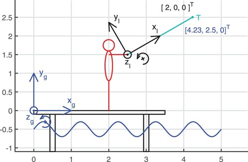
Mathematically, there are vectors from the two origins shown to the point T, expressed in terms of the base vectors $\mathbf{i},\mathbf{j},\mathbf{k}$ of the respective coordinate systems: (1a) $\begin{array}{rl}{\mathbf{p}}_{T(g)}={\mathbf{p}}_T& =[2.5+\sqrt{3},2.5,0{]}^T=(2.5+\sqrt{3}){\mathbf{i}}_g+2.5{\mathbf{j}}_g+0{\mathbf{k}}_g,\end{array}$(1a) (1b) $\begin{array}{rl}{\mathbf{p}}_{T(l)}={\overline{\mathbf{p}}}_T& =[2,0,0{]}^T=2{\mathbf{i}}_l+0{\mathbf{j}}_l+0{\mathbf{k}}_l.\end{array}$(1b) Linear algebra allows to speak of abstract vectors, irrespective of the coordinate representation, but this isn't very helpful for the software implementation. There we consider concrete vectors that are connected to (‘expressed in’, ‘using’) a coordinate system.

In an object oriented approach, coordinate systems aren't very lively objects. They are like sheets of squared paper, providing means for measuring distances and orientations.

• A coordinate system consists of a name, an origin $O=[0,0,0{]}^T$, unit vectors $\mathbf{i}=[1,0,0{]}^T,\mathbf{j}=[0,1,0{]}^T,\mathbf{k}=[0,0,1{]}^T$, and a length scale.

Design choices are to restrict attention to 3-dimensional space, using right-handed coordinate systems and $[\text{mm}]$ as the unit of length where possible. Cartesian coordinates, cylindrical coordinates and (generalised) curvilinear coordinates are used. Left-handed coordinates are needed sometimes when using mirroring between left and right wheels, to consider both sides with a single software implementation.

• A vector (3-vector) is a triplet $\mathbf{v}=[v_1,v_2,v_3{]}^T$ associated with the three coordinate axes of a coordinate system: $\mathbf{v}=v_1\mathbf{i}+v_2\mathbf{j}+v_3\mathbf{k}$.

In the software, the values $v_i$ are unrestricted ($\in \mathbb{R}$) in cartesian coordinate systems. In cylindrical coordinates ($\mathbf{v}=[r,\theta ,v_3{]}^T,v_3=x,y$ or z), $r\in {\mathbb{R}}_0^{+}$ and $\theta \in [0,2\pi )$.

Vectors can be set and read, scaled, and combined in different ways like adding and computing the dot and cross products. Further, they can be transformed from one coordinate system to another, using the mechanisms that are described below.

2.2. Notations for the coordinate reference

The different coordinate systems provide powerful means for preparing the inputs to CONTACT. They allow to prepare the wheel surface easily in wheel profile coordinates, transform to track coordinates for the 3-d contact search procedure including yaw, then transform further to contact local coordinates, describing the contact problems in normal and tangential directions. However, algorithms will fail if coordinate values are entered in one form where another form is expected. Therefore it's of paramount importance to be clear at all times on the reference system that is used. This is done in different ways.

• The coordinate reference is dropped at places where only a single coordinate system is relevant. For instance, when dealing with the internals of the CONTACT model, we simply use $[x,y,z{]}^T$ and $[p_x,p_y,p_z{]}^T$, according to the local contact coordinate system.

• At places where two coordinate systems are used, Shabana's notation is adopted [43], distinguishing between ‘global’ and ‘local’ coordinates, writing $[\overline{x},\overline{y},\overline{z}{]}^T$ to indicate a vector in local coordinates. This has a clear meaning without introducing confusion with other sub- or superscripts that are in use. The same is achieved using $[x,s,n{]}^T$ for contact local coordinates while using $[x,y,z{]}^T$ for the global track system.

• At places where more coordinate systems are needed, these are indicated by additional sub- or superscripts such as $[x_c,y_c,z_c{]}^T$ for contact local coordinates or $[x_w,y_w,z_w{]}^T$ for wheel profile coordinates.

• The reference to the coordinate system is put in parentheses when other subscripts are used as well, e.g. ${\mathbf{m}}_{cp(tr)}$ for a point ${\mathbf{m}}_{cp}$ expressed in track coordinates (tr).

2.3. Rotation matrices

Objects may have an orientation, such as the fishing rod in Figure 1. This orientation is expressed with respect to a coordinate system. For a person, for instance, the natural orientation may be to look into the direction of the positive x-axis, with the positive y-axis pointing to the left side and positive z-axis pointing upwards.

• A rotation matrix is a $3\times 3$ matrix $\mathbf{R}$ that describes orientation of an object through the direction cosines [43]. The columns of $\mathbf{R}$ may be viewed as the natural vectors $\mathbf{i},\mathbf{j},\mathbf{k}$ of the object, expressed in terms of the coordinate system used.

Rotation matrices are orthonormal, that is, each column has unit norm and is orthogonal to the other columns, such that ${\mathbf{R}}^T\mathbf{R}=\mathbf{I}$. The inverse of a rotation $\mathbf{R}$ is thus described by the transpose matrix ${\mathbf{R}}^T$.

Rotation matrices are used as the primary means of storing orientations in CONTACT, because they allow coordinate transformations to be implemented directly. The formulas by which this works depend on ones conventions:

• We use column vectors throughout and apply rotations by pre-multiplication,

• using right-handed coordinate systems,

• using the right-hand rule where counter-clockwise rotation is positive when looking from the positive side of an axis down to the origin.

Rotation matrices can be constructed from basic rotations, multiplied, transposed, and applied to a vector.

2.4. Euler angles

Euler angles are used in the input to CONTACT, particularly for the orientation of the wheelset with respect to the track.

• Euler angles are triplets $\{\varphi ,\psi ,\theta \}$ for roll, yaw and pitch, that describe the orientation of an object (point, coordinate system, body) via three successive rotations starting from the natural orientation.

Euler angles can be used in different ways, e.g. using intrinsic or extrinsic rotations, and in different ordering. One of their complications is the existence of singular configurations. In our work we adopt the roll–yaw–pitch convention throughout. This avoids singularities, as long as roll and yaw remain limited. Another complication of Euler angles is that they cannot be time-integrated, which isn't relevant to our application.

The basic rotations in ${\mathbb{R}}^3$, with roll, pitch and yaw angles $\varphi ,\theta ,\psi$, about the x-, y- and z-axes, are described using the matrices (2a) $\begin{array}{rl}\text{roll}:{\mathbf{R}}_x(\varphi )& \stackrel{def}{=}\left[\begin{array}{ccc}1& 0& 0\\ 0& c_{\varphi }& -s_{\varphi }\\ 0& s_{\varphi }& c_{\varphi }\end{array}\right]=\left[\begin{array}{ccc}1& 0& 0\\ 0& \cos (\varphi )& -\sin (\varphi )\\ 0& \sin (\varphi )& \cos (\varphi )\end{array}\right],\end{array}$(2a) (2b) $\begin{array}{rl}\text{pitch}:{\mathbf{R}}_y(\theta )& \stackrel{def}{=}\left[\begin{array}{ccc}{c}_{\theta }& 0& s_{\theta }\\ 0& 1& 0\\ -s_{\theta }& 0& c_{\theta }\end{array}\right]=\left[\begin{array}{ccc}\cos (\theta )& 0& \sin (\theta )\\ 0& 1& 0\\ -\sin (\theta )& 0& \cos (\theta )\end{array}\right],\end{array}$(2b) (2c) $\begin{array}{rl}\text{yaw}:{\mathbf{R}}_z(\psi )& \stackrel{def}{=}\left[\begin{array}{ccc}{c}_{\psi }& -s_{\psi }& 0\\ s_{\psi }& c_{\psi }& 0\\ 0& 0& 1\end{array}\right]=\left[\begin{array}{ccc}\cos (\psi )& -\sin (\psi )& 0\\ \sin (\psi )& \cos (\psi )& 0\\ 0& 0& 1\end{array}\right].\end{array}$(2c) Using the roll–yaw–pitch convention $\varphi \text{--}\psi \text{--}\theta$, rotations are carried out first about the x-axis, then about the new $z^{\prime }$-axis, and thirdly about the final $y^{″}$-axis. Such intrinsic rotations, about successive intermediate axes, are obtained by multiplying the basic rotations on original axes in reverse order. The final rotation matrix is then obtained as (3) $\begin{array}{rl}\mathbf{R}(\varphi \text{--}\psi \text{--}\theta )={\mathbf{R}}_{y^{″}}(\theta ){\mathbf{R}}_{z^{\prime }}(\psi ){\mathbf{R}}_x(\varphi )& ={\mathbf{R}}_x(\varphi ){\mathbf{R}}_z(\psi ){\mathbf{R}}_y(\theta )\\ & =\left[\begin{array}{ccc}{c}_{\psi }{c}_{\theta }& -s_{\psi }& c_{\psi }{s}_{\theta }\\ s_{\varphi }{s}_{\theta }+c_{\varphi }{s}_{\psi }{c}_{\theta }& c_{\varphi }{c}_{\psi }& -s_{\varphi }{c}_{\theta }+c_{\varphi }{s}_{\psi }{s}_{\theta }\\ -c_{\varphi }{s}_{\theta }+s_{\varphi }{s}_{\psi }{c}_{\theta }& s_{\varphi }{c}_{\psi }& c_{\varphi }{c}_{\theta }+s_{\varphi }{s}_{\psi }{s}_{\theta }\end{array}\right].\end{array}$(3) The value $\theta =0$ is relevant when considering a coordinate system that isn't affected by pitch rotation: (4) $\begin{array}{r}\mathbf{R}(\varphi \text{--}\psi )=\left[\begin{array}{ccc}1& 0& 0\\ 0& c_{\varphi }& -s_{\varphi }\\ 0& s_{\varphi }& c_{\varphi }\end{array}\right]\left[\begin{array}{ccc}{c}_{\psi }& -s_{\psi }& 0\\ s_{\psi }& c_{\psi }& 0\\ 0& 0& 1\end{array}\right]=\left[\begin{array}{ccc}{c}_{\psi }& -s_{\psi }& 0\\ c_{\varphi }{s}_{\psi }& c_{\varphi }{c}_{\psi }& -s_{\varphi }\\ s_{\varphi }{s}_{\psi }& s_{\varphi }{c}_{\psi }& c_{\varphi }\end{array}\right].\end{array}$(4) For Wang's method for the contact locus, a matrix shows up using the yaw–roll–pitch convention: (5) $\mathbf{R}(\psi \text{--}\varphi )=\left[\begin{array}{ccc}{c}_{\psi }& -s_{\psi }& 0\\ s_{\psi }& c_{\psi }& 0\\ 0& 0& 1\end{array}\right]\left[\begin{array}{ccc}1& 0& 0\\ 0& c_{\varphi }& -s_{\varphi }\\ 0& s_{\varphi }& c_{\varphi }\end{array}\right]=\left[\begin{array}{ccc}{c}_{\psi }& -s_{\psi }{c}_{\varphi }& s_{\psi }{s}_{\varphi }\\ s_{\psi }& c_{\psi }{c}_{\varphi }& -c_{\psi }{s}_{\varphi }\\ 0& s_{\varphi }& c_{\varphi }\end{array}\right].$(5)

2.5. Coordinate transformations

The combination of a vector with a rotation matrix is called a marker object. These markers facilitate transformations between different coordinate systems.

• A marker is a ‘point with orientation’ in terms of a base coordinate system: a position vector $\mathbf{o}$ plus rotation matrix $\mathbf{R}$.

In a way, markers define new, local coordinate systems, within the global base system. The origin of the local system is described using the vector ${\mathbf{o}}_{l(g)}$, from $O_g$ to $O_l$, in terms of global coordinates. The orientation is defined using a rotation matrix $\mathbf{R}$, of which each column expresses one of the local base vectors in terms of global coordinates, (6) ${\mathbf{R}}_{l(g)}=\left[\begin{array}{ccc}|& |& |\\ {\mathbf{i}}_{l(g)}& {\mathbf{j}}_{l(g)}& {\mathbf{k}}_{l(g)}\\ |& |& |\end{array}\right].$(6) This links the two systems together, allowing for the conversion of vectors between them. Combining equations (1b(1b) $\begin{array}{rl}{\mathbf{p}}_{T(l)}={\overline{\mathbf{p}}}_T& =[2,0,0{]}^T=2{\mathbf{i}}_l+0{\mathbf{j}}_l+0{\mathbf{k}}_l.\end{array}$(1b) ) and (6(6) ${\mathbf{R}}_{l(g)}=\left[\begin{array}{ccc}|& |& |\\ {\mathbf{i}}_{l(g)}& {\mathbf{j}}_{l(g)}& {\mathbf{k}}_{l(g)}\\ |& |& |\end{array}\right].$(6) ) it follows that (7a) $\begin{array}{rl}& \text{`to global'}:{\mathbf{p}}_{(g)}={\mathbf{o}}_{l(g)}+{\mathbf{R}}_{l(g)}{\mathbf{p}}_{(l)},\text{or}\mathbf{p}=\mathbf{o}+\mathbf{R}\overline{\mathbf{p}}\end{array}$(7a) (7b) $\begin{array}{rl}& \text{`to local'}:{\mathbf{p}}_{(l)}={\mathbf{R}}_{l(g)}^T({\mathbf{p}}_{(g)}-{\mathbf{o}}_{l(g)}),\text{or}\overline{\mathbf{p}}={\mathbf{R}}^T(\mathbf{p}-\mathbf{o})\end{array}$(7b) In the example of Figure 1, where the angle from ${\mathbf{i}}_g$ to ${\mathbf{i}}_l$ is ${30}^{\circ }$, (8) $\mathbf{R}=\left[\left[\begin{array}{c}0.87\\ 0.5\\ 0\end{array}\right]\left[\begin{array}{c}-0.5\\ 0.87\\ 0\end{array}\right]\left[\begin{array}{c}0\\ 0\\ 1\end{array}\right]\right],\mathbf{o}+\mathbf{R}\overline{\mathbf{p}}=\left[\begin{array}{c}2.5\\ 1.5\\ 0\end{array}\right]+\left[\begin{array}{c}1.73\\ 1\\ 0\end{array}\right]=\left[\begin{array}{c}4.23\\ 2.5\\ 0\end{array}\right].$(8) Markers can be constructed and modified in different ways, using translation and basic rotations. They are used to capture (store) the relative positions of the main objects in the geometry problem, and to transform vectors, grids, and other markers from one coordinate system to another.

Expressions that relate the local and global velocities of a point $\mathbf{p}$ on a body are obtained by taking the derivative of equation (7a(7a) $\begin{array}{rl}& \text{`to global'}:{\mathbf{p}}_{(g)}={\mathbf{o}}_{l(g)}+{\mathbf{R}}_{l(g)}{\mathbf{p}}_{(l)},\text{or}\mathbf{p}=\mathbf{o}+\mathbf{R}\overline{\mathbf{p}}\end{array}$(7a) ) with respect to time. (9) $\dot{\mathbf{p}}=\dot{\mathbf{o}}+\dot{\mathbf{R}}\overline{\mathbf{p}}+\mathbf{R}\dot{\overline{\mathbf{p}}},\text{with}\dot{\mathbf{R}}\overline{\mathbf{p}}={\mathit{\omega }}_l\times (\mathbf{R}\overline{\mathbf{p}})=\mathbf{R}({\overline{\mathit{\omega }}}_l\times \overline{\mathbf{p}})\text{and}\mathbf{R}\dot{\overline{\mathbf{p}}}=\mathbf{R}\overline{\mathbf{v}}.$(9) This shows how the total velocity ${\mathbf{v}}_p=\dot{\mathbf{p}}$ of a point with respect to the global origin may be decomposed into three contributions:

1. Rigid body translation, ${\mathbf{v}}_l=\dot{\mathbf{o}}$, of the local system with respect to the global origin;

2. Rigid body rotation, ${\mathit{\omega }}_l$, of the local system with respect to the global system, at an arm $\mathbf{R}\overline{\mathbf{p}}$ of the point with respect to the local origin;

3. Flexible body deformation, motion of the point within the local system, ${\overline{\mathbf{v}}}_p=\dot{\overline{\mathbf{p}}}$, at the current orientation $\mathbf{R}$ of the local system.

Detailed information on the relations between angular velocities ${\mathit{\omega }}_l,{\overline{\mathit{\omega }}}_l$ and the derivative $\dot{\mathbf{R}}$ is given in [43, § 2.4–2.5].

2.6. Grids and grid functions

Primary work horses in our implementation are grids and grid functions.

• A 1-d grid (curve, profile) is an ordered list of points $\{{\mathbf{x}}_i\},i=1,\dots ,n_1$ or $\{{\mathbf{x}}_j\},j=1,\dots ,n_2$ in terms of a given coordinate system.

• A 2-d grid (mesh, surface) is a structured set of points $\mathcal{G}=\{{\mathbf{x}}_{ij}\},i=1,\dots ,n_1,j=1,\dots ,n_2$ in terms of the coordinate system used.

1-d grids are implemented in CONTACT using 2-d grids with either $n_1=1$ or $n_2=1$. Further, all ${\mathbf{x}}_{ij}=[x_1,x_2,x_3{]}_{ij}^T$ are points in 3-d space. Grids can be flat but don't have to be, flat grids can be aligned with coordinate directions but may also be tilted.

Rail profiles are implemented as planar curves in the Oyz plane, using $n_1=1$, $x_j\equiv 0$, with $n_2$ points in y-direction. Wheel profiles are defined using cylindrical coordinates with $x_j\widehat{=}{\theta }_j\equiv 0,z_j\widehat{=}{r}_j-r_{nom,w}$. Generic conversion routines are provided to convert to cartesian coordinates, assuming the wheel is a body of revolution. The contact locus on the wheel is a generic space curve, ${\mathbf{x}}_j=[x_j,y_j,z_j{]}^T$, with $x_j\ne 0$.

A grid is called ‘uniform’ in CONTACT if the coordinates can be expressed as $x_{ij}=x_0+i\delta x$ (same for all j) and $y_{ij}=y_0+j\delta y$ (same for all i), using fixed steps $\delta x,\delta y$, with $z_{ij}=const$. (This is a restricted definition of uniformity; other forms of uniformity could be recognised also.) Non-uniform grids are called ‘cylindrical’ or ‘curvilinear’. Cylindrical grids can be transformed into cartesian coordinates. Cartesian coordinates can be transformed from one origin and orientation to another, using the to-global and to-local operations of equations (7a(7a) $\begin{array}{rl}& \text{`to global'}:{\mathbf{p}}_{(g)}={\mathbf{o}}_{l(g)}+{\mathbf{R}}_{l(g)}{\mathbf{p}}_{(l)},\text{or}\mathbf{p}=\mathbf{o}+\mathbf{R}\overline{\mathbf{p}}\end{array}$(7a) ) and (7b(7b) $\begin{array}{rl}& \text{`to local'}:{\mathbf{p}}_{(l)}={\mathbf{R}}_{l(g)}^T({\mathbf{p}}_{(g)}-{\mathbf{o}}_{l(g)}),\text{or}\overline{\mathbf{p}}={\mathbf{R}}^T(\mathbf{p}-\mathbf{o})\end{array}$(7b) ).

One main purpose of uniform grids is to define the ‘contact grid’, in the Oxy-plane, aligned with contact-local x, y-coordinate axes. The contact grid points are associated with the centres of rectangular elements, with a secondary grid of corners induced at ${\mathbf{x}}_{ij}+[\pm \delta x/2,\pm \delta y/2,0{]}^T$. The regular structure allows for quick determination of the elements in which points are located, as needed in interpolations.

• A 1-d grid function is a function $f:\mathcal{G}\to \mathbb{R}$, assigning scalar values $f_{ij}$ to each grid point ${\mathbf{x}}_{ij}$ of a grid $\mathcal{G}$.

• A 3-d grid function is a function $\mathbf{f}:\mathcal{G}\to {\mathbb{R}}^3$, assigning triplets $[f_1,f_2,f_3{]}_{ij}^T$ to each grid point ${\mathbf{x}}_{ij}$ of a grid $\mathcal{G}$.

Grid functions are used to store all kinds of information like surface heights $h_{ij}$, surface tractions ${\mathbf{p}}_{ij}$, elastic displacements ${\mathbf{u}}_{ij}$, or mask arrays $m_{ij}$, indicating the status of each point. 3-d grid functions typically contain vectorial values, relative to the coordinate axes of an underlying coordinate system.

In the implementation, the two indices ij are collapsed into a single index $I=i+(j-1)n_1,I=1,\dots ,n_{tot}=n_1{n}_2$.

Using a different view point, grids may be considered as grid functions themselves. In this view, a grid's essential information consists of the indices, $\mathcal{G}=\{ij\}$, making the coordinates a grid function $\mathbf{x}:\mathcal{G}\to {\mathbb{R}}^3$. This view relates to the concept of index sets as elaborated in [47].

2.7. Splines and interpolations

Basic 1-d linear interpolations are provided in CONTACT using a generic routine for non-equidistant input data that may be given in ascending or descending order. Multiple interfaces are built on top of this routine, for scalar, array, or grid outputs. Similarly, a single routine is constructed for the computation of interpolation weights for 2-d curvilinear to uniform grid interpolation, with multiple wrappers for different forms of the actual data.

Smooth interpolation of curves is provided via cubic splines.

• A 1-d simple spline for a 1-d tabulated function $\{t_i,y_i\}$ approximates the underlying function $y=y(t)$ with piecewise cubic sections with parameter t.

Simple splines are called ‘interpolating’ when the tabulated points are retrieved at appropriate parameter values, or ‘smoothing’ if the input points are not contained in the resulting curve. Cubic splines are stored using the coefficients $[a_0,a_1,a_2,a_3{]}_i$ for all table segments, of polynomial terms $t^0,t^1,t^2,t^3$, respectively, related to the ppform of de Boor [48].

• A 1-d parametric spline for a 1-d grid $\{[x_j,y_j,z_j{]}^T\}$ approximates the underlying space curve as $(x(s),y(s),z(s))$ with s the arc length parameter.

Parametric splines are composed of three simple splines with the same parametrisation.

Parametric spline objects can be computed, copied, trimmed, shifted, rotated, and evaluated in direct and indirect ways. Direct evaluation gives the profile positions and inclinations at specified s-positions. Indirect evaluation takes the desired y-values as input, locates the corresponding s-positions in the spline function, and delivers x, y, z and their partial derivatives like $\mathrm{\partial }y/\mathrm{\partial }s$ or $\mathrm{\partial }z/\mathrm{\partial }y$ as the output values.

3. Steps used to solve the contact geometry problem

3.1. Scope of the problem

CONTACT aims to solve contact problems for a wide range of configurations, for vehicle dynamics as well as stand-alone users, without placing much burden on the user. This appeared challenging in case of the wheel/rail geometry problem, that arises in many different ways.

• Wheel and rail profiles are provided in a wide range of forms, from constant radius arcs on technical drawings, to measured, worn profiles in various formats. These alternative forms may need different kinds of preparations (smoothing, alignment, unit conversion, positioning in the track), and may need or allow for different algorithms for the contact detection.

• The position of a wheel with respect to a rail may be specified in different ways, using an ideal design track or from measured data, with different conventions for signs and angles.

• Stand-alone wheel/rail contact investigation has different points of departure than vehicle dynamics simulation. Vehicle dynamics typically needs the contact forces at precisely specified states of wheel and rail, while stand-alone users typically want to specify certain total forces or moments. This adds additional balance equations to the problem, typically concerning a whole wheelset instead of a single wheel on a rail.

Considered as a software problem, this gives a very informal and unclear requirements specification: what should or should not be implemented? How can the problem be specified by a user in a detailed yet convenient way? A solution is implemented in CONTACT, that relies on the following design decisions for the software implementation:

• Rigorous choices are made regarding the coordinate systems and the use of the multibody formalism for their manipulation;

• Wheel and rail profiles are read from a wide range of formats, and brought into canonical form before starting the actual calculations;

• The geometry problem is analysed twice; first for the location of contact patches, and then for the local geometry of the contact patches;

• Surfaces are constructed as grids in local coordinates, transformed, and evaluated using interpolation, rather than transforming the equations by which the surfaces are defined.

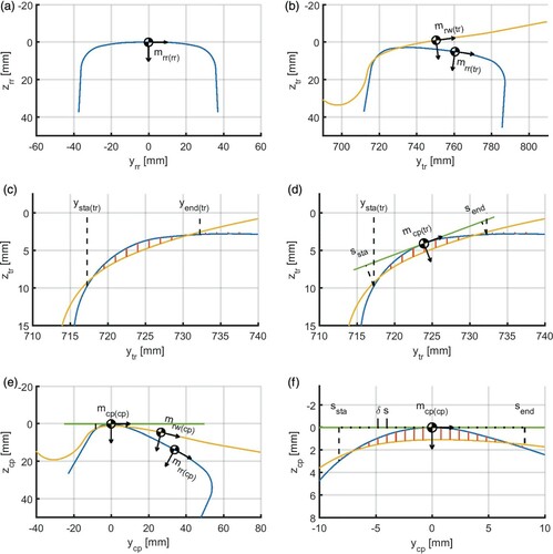
The steps that are used are shown pictorially in Figure 2, and are elaborated in the following sections.

Figure 2. Main steps used for wheel/rail contact geometry processing, using markers and associated coordinate systems.

3.2. Wheel and rail profiles

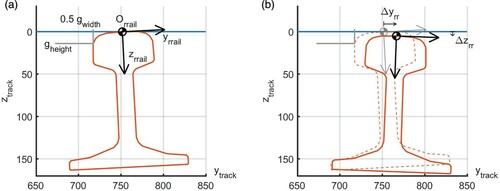
Wheel and rail profiles are read from various formats, using a wide range of different conventions. They are transformed into a canonical form, showing profiles for the right side of the track, using right-handed coordinates with z positive downwards (Figure 2(a)).

Up/down and left/right mirroring are used as needed. The profiles could further be scaled, shifted, trimmed, and so on, and smoothing may be applied. A marker is placed at the zero position in the profiles, defining the wheel and rail profile coordinate systems, and the spline representation is built. These preparations simplify the further processing: providing information in a consistent way to the actual solvers, reducing the number of options that must be considered there.

3.2.1. Requirements for rail profiles

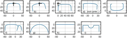
The variety of rail profiles is illustrated in Figure 3.

• Rail profiles can be provided before (a) or after applying the rail cant angle (b).

• The profile coordinate origin can be chosen at the top of the rail (a), at the gauge face (c), or anywhere else (d, f).

• The profiles could be measured for the rail on the left side of the track (d) or for the right side (b).

• The profiles could be measured with z positive upwards (e) or downwards (a).

• Lateral positions could be increasing monotonically (a), or could be decreasing at some points (d, e), creating multi-valued functions.

• Rails could consist of multiple sections, particularly at switches and crossings (f).

• For testing purposes, rails could be defined as circular arcs (g) or planar sections (h).

• The side face of the rail could be too small for the gauge width computation (h).

• The biggest width needed for the gauge width computation may occur above the gauge measuring height (d).

• The highest part of the rail need not be the most relevant for contact analysis (i).

• Profiles may contain sharp corners (i), that must be dealt with appropriately in operations like smoothing and interpolation.

• The profiles could be measured in $[\text{mm}]$, $[\text{m}]$ or $[\text{in}]$, etc.

Figure 3. Variety of rail profiles that should be supported.

3.2.2. Requirements for wheel profiles

A variety of wheel profiles is shown in Figure 4.

Figure 4. Variety of wheel profiles that should be supported.

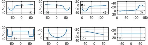
• Profiles can be given for right (a) or left wheels (b).

• The profile coordinate origin can be placed at the tape circle line (a, b), at the flange back (c), or anywhere else (d).

• The profiles can be given with z positive downwards (a, b, c) or upwards (d).

• A wheel may have one (a–d), two (e), or no flanges (f–h).

• For testing purposes, wheels may be defined with a circular cross-section (f) or as a flat/conical section (g).

• Idealised two-dimensional contacts require a logarithmical drop at the sides (h), to avoid pressure concentration [49,50], [51, p.134].

Wheel profiles can be narrower or wider than the rail profile. In case of a grooved rail profile (Figure 3(i)), a narrow circular wheel (Figure 4(f)) may have its lowest z-values larger than the lowest z on the rail. In that case, the wheel profile may not be extended by constant extrapolation.

3.2.3. Canonical form, mirroring

Users want to be able to define a profile just once and then use this definition on both sides of a rail vehicle. Likewise, it is beneficial for programmers to concentrate on a single geometrical configuration, that could either be for the left or right side of the track, yet avoid switching between sides. This way, the flange will be found at the same position, angles will be in a consistent range, and so on, allowing to familiarise and memorise the values. Positive values that should be negative are then spotted much quicker, the same for clockwise and counter-clockwise rotations. Programming errors are detected and corrected more easily, and prevented by standardisation.

Different conventions are possible for the reference position on a profile (on the side or at the top of the rail), for the orientation (before or after cant rotation), for the mirroring (left or right side), and ordering of the points (low-to-high, high-to-low).

• We let the reference position in the rail profile be defined freely by the user. We place a marker at this reference position and use this to move the rail around in the track system.

• We focus on the wheel/rail pair on the right side of the track. Problems for the left side are mirrored in the plane $y_{tr}=0$. This flips the sign on y-components of positions, velocities, tractions, and forces. Rotations are affected about the x- and z-axes, affecting angular orientations and velocities and corresponding moments.

Optional mirroring is provided for cases where left side profiles are given on input.

3.3. Profile smoothing and spline interpolation

Measured worn profiles may exhibit small grooves and ridges that have a strong influence on the contact results. The normal contact problem is particularly sensitive to variations in the undeformed distance, resulting in irregularly shaped contact patches, composed of multiple disconnected sections, with consequent variations in the contact pressures. Such irregularities in the results may be desired in some cases, for detailed studies, but are typically seen as unwanted effects. Different results would be obtained for profile measurements that are taken close together on the same wheel or same rail. The fluctuations will turn out differently with every other instance of the profiles. Profile smoothing may be used to attenuate the most rapid fluctuations.

Profile smoothing can be achieved using cubic smoothing splines, as discussed for instance in [48,52–54]. A particularly convenient description that we used was given by Pollock [55]. For a given set of data points $\{s_i,y_i\}$ and weights ${\sigma }_i,i=1\cdots n$, this constructs the spline function $Y(s)$ that minimises the value of (10) $L=\sum _{i=1}^n{\left(\frac{y_i-Y(s_i)}{{\sigma }_i}\right)}^2+\lambda {\int }_{s_1}^{s_n}{(Y^{″}(s))}^2\text{d}s$(10) The first term describes the deviation from the input data, the latter the smoothness of the spline function. The parameter λ concerns the level of smoothing, with no smoothing at all for $\lambda =0$ and using a linear function $Y(s)$ for $\lambda \to \mathrm{\infty }$.

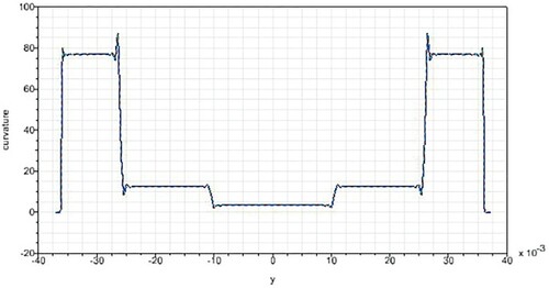
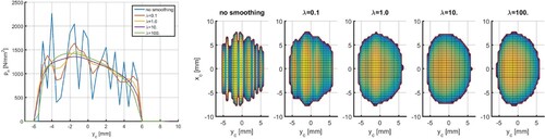
A possible drawback is that spline smoothing tends to exhibit overshoots in curvature at places where the input curvature jumps from one to another value. This is illustrated in Figure 5 for the UIC60 profile that consists of 300, 80 and 13 mm radius arcs joined together. This issue requires some special attention for algorithms that use the curvatures, for instance to make a Hertzian approximation.

Figure 5. Curvature of new UIC60 rail profile obtained from smoothing spline interpolation.

Other algorithms for smoothing are the Savitzki-Golay approach [56] or Lowess and Loess filters. An interesting idea is to use optimisation of an objective function that includes curvature, as proposed in the method of ‘minimum curvature variation’ [57].

Another way to approach the smoothing problem is by fitting of circular arcs to segments of the profile data. This is used in the Universal Mechanism software [pers.comm]. This fitting is intricate for profile segments that have low curvature, where it's difficult to decide whether the curve centre should be moved to the left or the right side of the curve. This ill-posedness can be avoided by reformulation of the problem, using the curvature instead of the curve radius as optimisation variable [58], by which low curvature segments approach 0 from positive and negative sides.

A topic related to smoothing concerns profile interpolation. Even if the input data themselves are obtained from a smooth profile, a rough profile may result if interpolation is used in the wrong way. Linear interpolation creates facets that distort the results if the contact grid has higher sampling than the input profile. This is illustrated in Figure 6 for a case where the profiles are given with steps of about 1 mm, using 0.2 mm steps in CONTACT. This facetting is avoided using higher order interpolation, as provided by cubic spline interpolation.

Figure 6. Spikes in the computed pressures $p_n$ due to facets in the undeformed distance function. Picture thanks to K. Oldknow [pers.comm].

3.4. Track geometry and wheelset definition

A second step in the preparations concerns the positioning of the wheel and rail profiles with respect to each other (Figure 2(b)). Different ways of specification may be used that each have their own benefits in different circumstances. Absolute positioning of rails can be used, with respect to a global coordinate system, especially in the case of a design track layout with track irregularities and/or rail bending. Alternatively, the relative positions of the rails may be used, using the gauge width measured at some height below the plane resting on the top of the rails. This is especially practical for measured track data, where the absolute position may not be accessed easily.

The input to CONTACT has been designed to strike a balance between the different cases. This is done with the aid of a virtual ‘wheelset’ and ‘track’, to describe the geometry in terms familiar to the user, using two wheels and two rails. The simulation of a test rig is also supported, with rollers replacing the rails, as well as a configuration with a single wheel on a rail. Currently, the two sides are considered as separate wheel/rail contact problems. CONTACT does not yet provide for the interactions between the two wheels, adjusting the roll angle for instance, to satisfy an equilibrium equation.

3.4.1. Track geometry

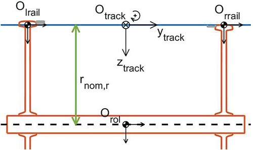
CONTACT does not consider gravity and the corresponding vertical direction. The basis of working is the track plane, defining its own vertical direction. A marker ${\mathbf{m}}_{tr}$ is introduced as shown in Figure 7 (right). In rail vehicle dynamics, the track origin may be placed at the point on the track curve closest to the wheelset centre of mass (CM), see e.g. [36]. This position is denoted here as $s_{ws}$, with s ($s_1$, longitudinal) the parameter used to describe the track curve. The $x_{tr}$ direction is aligned with the track centre line, $y_{tr}$ is the lateral direction, positive to the right, by which $z_{tr}$ is positive downwards.

Figure 7. Left: track viewed in world-coordinates (not used in CONTACT), with track inclination (elevation) angle ϕ (adapted from [31]). Right: definition of the track coordinate system, at the centre of the plane resting on the (inclined) rails in initial (design) configuration.

The right rail profile is placed in the track using the gauge computation, defining a marker ${\mathbf{m}}_{rr(tr)}$. This is initialised at $\{\mathbf{0},\mathbf{I}\}$, rotated by the rail cant angle, if not included in the profile itself, then shifted upwards and to the right to touch precisely the track plane and gauge stop as shown in Figure 8 (left). The left-most point of the profile is used for $z_{rr(tr)}\in [0,g_{height}]$, as suggested by the gauge-stop in the figure. An alternative choice is to evaluate the profile at $z_{rr(tr)}=g_{height}$. This is the convention used in the VAMPIRE software. This affects the positioning of rails as shown in Figure 3(d), where the left-most point lies above the gauge measuring height.

Figure 8. Left: initial (design) placement of the right rail profile in the track system, with positive cant angle, using gauge width and gauge measuring height. Right: actual (current) configuration with rotation $\mathrm{\Delta }{\varphi }_{rr}$ and displacements $\mathrm{\Delta }{z}_{rr},\mathrm{\Delta }{y}_{rr}>0$.

Next, track irregularities may be defined that displace the rails with respect to their initial (design) positions and orientations, see Figure 8 (right), see [27, § 4.2] for a further specification. These rail irregularities may be static/permanent, but may be due to track flexibility too. In such a case, the corresponding velocities $v_{rr}=\mathrm{\Delta }{\dot{y}}_{rr},\dots$ may be specified also, affecting the creep calculation [59,60].

3.4.2. Roller rig configurations

For the simulation of roller rigs, it is assumed that the roller axle is fixed in a frame, unable to move except for rotation about its axle. Track coordinates are used largely similarly as above for wheelset on track configurations, with slight differences as indicated in Figure 9:

• The track plane is aligned with the rollers' axle, at the nominal roller radius $r_{nom,r}$ above the rollers' centre of mass;

• The profile markers for the rollers are placed directly in the track plane, without up/down shifting to make the profiles touching the track plane. The z-values in the profile are thus interpreted as variations of the rolling radius with respect to $r_{nom,r}$.

Figure 9. Definition of track coordinates for the simulation of a roller rig: aligned with the rollers' axle, at a distance $r_{nom,r}$ above the rollers' centre of mass.

The gauge computation is used for the lateral positioning of the profiles in the initial (design) configuration. The profiles may then be rotated and displaced by deviations for irregularities and flexible bending. This feature may also be used to describe the motion of the roller rig as a whole, relative to the frame in which it is contained.

3.4.3. Wheelset geometry

The geometry of the wheelset is defined using the flange back distance $d_{flng}$, the $y_{rw}$ location of the flange back in wheel profile coordinates, and the nominal radius $r_{nom,w}$ (Figure 10, left). These are used to set the wheel profile marker at ${\mathbf{x}}_{rw}=[0,d_{flng}/2-y_{fbpos},r_{nom,w}{]}^T$ with respect to the wheelset marker, in the initial (design) configuration. Flexible wheelset deviations may then be defined that displace the wheel profile with respect to its design position and orientation. Increments may be specified for all six position and orientation variables to support axle and wheel bending and torsion. The corresponding velocities may be specified as well.

Figure 10. Left: illustration of wheelset geometry parameters. Right: wheelset (CM) position and orientation with respect to the track system.

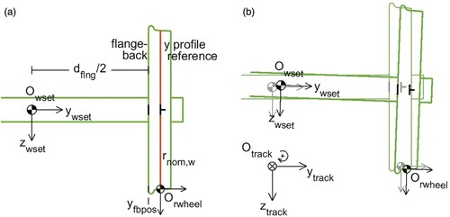
Next, the wheelset marker is defined, ${\mathbf{m}}_{ws}$, capturing the wheelset position and orientation with respect to the track frame (Figure 10, right). The position of a wheelset is characterised by the position of its centre of mass along the track curve ($s_{ws}$), which is largely irrelevant to CONTACT, and the position and orientation with respect to the track reference. The orientation is defined with Euler angles in roll–yaw–pitch convention: starting with the axle parallel to the $y_{tr}$-direction, the wheelset is rolled about its x-axis by ${\varphi }_{ws}$, then yawed by ${\psi }_{ws}$ about the new z-axis and then pitched by ${\theta }_{ws}$ about the axle, i.e. the new y-axis. After this the wheelset is shifted to its position $[0,y_{ws},z_{ws}-r_{nom,w}{]}^T$.

Using the markers ${\mathbf{m}}_{rw}$ and ${\mathbf{m}}_{ws}$ with suited local-to-global transformations, these yield the final position of the wheel profile in the track frame. The rail profile is positioned similarly using the rail profile marker, such that the two profiles can be plotted together in a single coordinate frame. This then provides the basis for the contact geometry problem (Figure 2(b)).

3.5. Locating the contact patches

The contact geometry is analysed in track coordinates, using the vertical wheel and rail surface positions, $z_{rr(tr)}-z_{rw(tr)}<0$. This gives the virtual interpenetration of the profiles, producing the potential extent of the contact patches along the way (Figure 2(c)). The ‘geometrical point of contact’ or ‘initial contact position’ is obtained at the location of maximum interpenetration. Multiple contact patches may be detected. Contact patches that lie close together may be joined, to include interactions between them in the actual contact solution.

Two different methods are implemented for the contact location: a brute-force, grid based approach, cf. [35], and a refined approach on the basis of the contact locus [28,32]. The grid based approach is easily understood and implemented for generic situations, including the yaw of the wheelset for instance, and for a wheel on a roller. It can be generalised further to corrugated rails, wheel flats, and wheels with polygonisation. This method is discussed further in this section.

The idea of the contact locus approach is to restrict the search to a 1-d curve instead of a 2-d surface. This is done using some analytical derivations that rely on the smoothness of the wheel and the rail. This is explained furter in Section 4, where the method is extended to wheel-on-roller configurations.

The grid based approach starts by defining a ‘reasonable arc’ on the wheel profile that should encompass the contact, typically $\theta =[-7^{\circ },7^{\circ }]$ with respect to the lowest point on the wheel. This arc is divided into a hard-coded, somewhat arbitrary number of $n_1=231$ slices. Considered as a brute-force method, little has been done on optimisation. This is suggested as a topic for further research.

The wheel profile is revolved around its axle creating a surface in cylindrical coordinates, converted to a cartesian surface in wheel profile coordinates, $\{x_i,y_i,z_i{\}}_{(w)}$, and transformed next to track coordinates. Note that these steps are provided directly by the software foundation, e.g.

A uniform ‘gap mesh’ is then defined in track coordinates for the whole width of the rail, using the range $x=[min(x_{i(tr)}),max(x_{i(tr)})]$ obtained from the wheel surface.

The 1-d rail profile is converted to track coordinates and computed at the $y_j$ of the gap mesh using spline evaluation. For wheel–rail contact, this is then extruded in x-direction to form a 2-d surface; for wheel–roller contact, the profile is revolved around it's axle and evaluated at the $x_j$ positions of the gap mesh. The bounding boxes of wheel and rail surfaces are checked. If there's no overlap then the user may have specified inappropriate positions or dimensions, such as the gauge width $g_{width}$ or flange-back position $y_{fbpos}$, else one or two profiles may need to be mirrored.

The z-values of the wheel surface are then interpolated to the gap mesh using 2-d bilinear interpolation, and the gap is formed as the difference $z_{r(tr)}-z_{w(tr)}$. All the local minima of this function are determined and recorded in a list. They are processed one by one, each time taking the one with largest interpenetration, defining a contact patch, and removing all the local minima contained in the patch. Once this list is exhausted, a new list of contact patches is formed. This may be sorted by lateral position, connected to a previous time-step, and may further be processed with respect to contact patches that lie close together.

The inputs to these calculations are the wheel and rail at their actual positions, including yaw, providing a 3-d contact search algorithm. The outputs are zero or more contact patch objects, and the overall minimum gap and corresponding curvatures that are determined also. Each contact patch consists of a contact reference marker, and the appropriate sizes for the potential contact area. The minimum gap value and the curvatures are used if the total force is prescribed and no contact occurs in the initial configuration. Solving a Hertzian problem, an appropriate value may then be obtained for the wheelset vertical position.

3.6. Contact grid definition

The definition of the contact grid needs information derived from the gap function, and is therefore implemented together with the location of the contact patches (Figure 2(d)).

The origin of the contact local coordinate system is traditionally placed at the initial contact position or geometrical point of contact [31,61,62]. Inspired by SIMPACK [38], we advocated for an alternative choice [42], keeping the origin more centred in asymmetric geometries. When using the grid based approach, this uses the mid-point of the interpenetration area, defined in a weighted sense, with the gap values $g(x,y)$ used as weights. (11) $[x_{tr},y_{tr}{]}_{cwgt1}={\int }_{g<0}[x,y]g(x,y)\text{d}x\text{d}y/{\int }_{g<0}g(x,y)\text{d}x\text{d}y.$(11) Experiments reported in [44] show that quadratic weights work somewhat better, and that it's desired to use an averaged surface inclination: (12) $[x_{tr},y_{tr},{\alpha }_{tr}{]}_{cwgt2}={\int }_{g<0}[x,y,\alpha ]g^2(x,y)\text{d}x\text{d}y/{\int }_{g<0}{g}^2(x,y)\text{d}x\text{d}y.$(12) Here ${\alpha }_{tr}$ is the surface inclination of the rail profile with respect to the track marker. For the contact locus approach this averaging is implemented using a quadratic approximation $g(t;y)=c(y)+a(y)t^2$. The minimum value $c(y)$ is the negative gap value found at the locus position $x_{lc}(y)$. The coefficient $a(y)$ comes from the curvature $a(y)=1/2r(y)$, and $t=x-x_{lc}$. This is the curvature in overall $z_{tr}$-direction, unaffected by the contact angle.

The rail profile is interpolated at $y_{tr}^{cwgt2}$ to get the corresponding $z_{tr}$-value, defining the contact reference position on the rail. The surface inclination could be obtained from the spline, and used to set the contact reference angle ${\delta }_{cp(tr)}$, the rotation from track z to local n-direction. A different choice is to use ${\alpha }_{tr}^{cwgt2}$, representing the average over the contact, improving the fit to conformal computations in a large set of test-cases [44]. Planar contact coordinates are then introduced by defining the marker ${\mathbf{m}}_{cp(tr)}$, with origin at the reference position and orientation using the contact reference angle.

The extent of the interpenetration region is obtained first in the horizontal $(x_{tr},y_{tr})$ plane using the gap function. The corresponding z-values are obtained from the rail profile. The desired size of the potential contact size $[s_{sta},s_{end}]$ is computed using temporary markers ${\mathbf{m}}_{sta}$ and ${\mathbf{m}}_{end}$, defined in track coordinates, then transformed into planar contact coordinates. The contact grid is defined in the contact plane, with requested step sizes $\delta x\times \delta s$, with a grid point placed at the contact origin. The number of grid points in each direction is computed large enough to encompass $s_{sta}$ and $s_{end}$, and similarly for the x-direction.

3.7. Combination of contact patches

For two contact patches that lie close together, there are interactions between their respective surface tractions and elastic deformations. The pressures on one patch typically reduce the amount of interpenetration found on the other [63], which reduces the pressures needed to satisfy the contact conditions. These interactions can be included in CONTACT by solving the patches in one go, using an enlarged potential contact area.

In principle, it's possible to combine all contact patches together into a single contact calculation. In the planar contact approach adopted in this paper, this needs a compromise for the contact reference angle: a single contact plane must be selected that strikes a balance between the actual contact angles found at different locations. This may introduce bigger approximation errors than when the interactions would be neglected. Therefore, a strategy is used that combines patches conditionally, on the basis of the mutual distance between adjacent patches, and on the change in contact angle.

Switching between combination or separation of adjacent patches may cause discontinuities in the numerical results at slight perturbations of input parameters. This is a concern for the solution of equilibrium equations such as a prescribed vertical force. These jumps may also introduce spurious, high-frequency oscillations in multibody simulations that are unphysical, and that should be prevented as much as possible [64,65].

A blending approach is introduced to mitigate some of the jumps, using two threshold values $d_{comb}\le d_{sep}$ for the distance d between their interpenetration areas and a third threshold ${\alpha }_{sep}$ for the angle difference. Two patches are processed separately when $|{\alpha }_{cp1}-{\alpha }_{cp2}|\ge {\alpha }_{sep}$ or when $d\ge d_{sep}$. Else, the patches are combined fully when $d\le d_{comb}$. In between, $d_{comb}\le d\le d_{sep}$, the patches are combined with interactions scaled by a factor θ: (13) $\theta ={\left(\frac{d_{sep}-d}{d_{sep}-d_{comb}}\right)}^{0.8}.$(13) This factor θ is applied inside CONTACT's solution algorithms by splitting the pressure array $p_n$ into parts for different sub-patches, computing elastic deformations u separately with influence coefficients A, and combining as follows: (14) $\left[\begin{array}{c}{u}_{1,1}\\ u_{2,1}\end{array}\right]=A\left[\begin{array}{c}{p}_1\\ 0\end{array}\right],\left[\begin{array}{c}{u}_{1,2}\\ u_{2,2}\end{array}\right]=A\left[\begin{array}{c}0\\ p_2\end{array}\right],u=\left[\begin{array}{c}{u}_{1,1}+\theta u_{1,2}\\ \theta u_{2,1}+u_{2,2}\end{array}\right].$(14) This extends the traditional formula ‘u = Ap’ as shown e.g. in [44, § 2.7]. The coefficient 0.8 in Equation (13(13) $\theta ={\left(\frac{d_{sep}-d}{d_{sep}-d_{comb}}\right)}^{0.8}.$(13) ) was found to give a reasonably smooth transition in one case that was studied in detail. Further research is needed on this, along with suitable choices for $d_{comb}$ and $d_{sep}$ in relation to total forces, material parameters and geometry of the problem.

3.8. Undeformed distance calculation

With the contact patches identified in the previous steps, defining markers and grids for the contact computations, the next step concerns the undeformed distance calculation. This is achieved by computing the wheel and rail surfaces in wheel and rail coordinate systems, then transforming the problem to the local coordinate system (Figure 2(e)). Using the appropriate software routines, we may sample the wheel profile as a body of revolution, place the points in the track frame, view the same in terms of contact coordinates, and use interpolation to get the heights at the contact grid (Figure 2(f)).

The steps used for the undeformed distance look much alike the steps used to determine the gap function. One difference is that the undeformed distance is analysed in contact coordinates, using surface heights $n_{r(cp)}-n_{w(cp)}$, evaluated at the contact grid positions. A second issue comes from multi-valuedness of the surface heights when the profile is viewed from a large angle, e.g. at $y_{cp}=50$ in Figure 2(e). This can happen in the overall z-direction as well (Figure 3(d, e)), but can be removed in those cases by restricting the acceptable profiles or discarding points where ‘fold-back’ occurs. When forming the undeformed distance, the multi-valuedness is inherent in the problem description. It is resolved by trimming the profiles, using the extent $[s_{min},s_{max}]$ of the contact grid.

One further difference with the previous calculation of the gap function, is that the undeformed distance function is needed with higher precision. This is achieved by evaluating the wheel and rail profile splines at the sampling density of the contact grid, followed by bilinear interpolation. Bi-cubic interpolation has been implemented as well, cf. [53, § 3.6], but the added benefits seem low compared to the added computations. Two-dimensional splines could also be useful, providing bi-cubic interpolation in a different way.

The calculation of the wheel surface heights $n_{w(cp)}$ uses a bounding box as a basis for the computation. This is computed using four markers at the corners of the contact grid, defined in track coordinates, transformed to wheel profile coordinates using to-local operations. This gives the range of $y_w$ values of relevance to the contact grid. This range is mapped to arc-length parameters $s_w$ on the wheel, divided into steps according to the contact grid spacing, and used to trim and re-sample the wheel profile as needed for the undeformed distance calculation. This profile is then revolved around its axle and evaluated at the appropriate range of $x_w$ with sampling $\delta x$ of the contact grid. From there the surface is known as $\{x_i,y_i,z_i{\}}_{(w)}$ covering the contact grid with sufficient resolution, and is transformed easily into $\{x_i,s_i,n_i{\}}_{(cp)}$.

3.9. Calculation of the creepages between wheel and rail

A final step concerns the determination of the creepages between the wheel and the rail. These are defined as the velocity of the surface of the upper (rail) body relative to that of the lower (wheel), evaluated at the origin of the local coordinate system, scaled by the rolling velocity V. There are three creepages, $\xi ,\eta ,\varphi$, for the velocity differences in longitudinal and lateral directions, $x=x_c,s=y_c$, and for the rotation about the normal direction $n=z_c$. Using P for the contact reference point on the rail or roller, and Q for the corresponding point on the wheel, the formulas are: (15) $\xi =\frac{v_x}{V}=\frac{v_x^P-v_x^Q}{V},\eta =\frac{v_s}{V}=\frac{v_s^P-v_s^Q}{V},\varphi =\frac{{\omega }_n}{V}=\frac{{\omega }_n^P-{\omega }_n^Q}{V}.$(15) These creepages approximate the local kinematic motions using a simplified form, $\mathbf{w}=[\xi -\varphi s,\eta +\varphi x{]}^T$, with rigid slip function $\mathbf{w}$. This approximation is improved upon in the conformal approach, by computing velocity differences at every point of the potential contact [44].

The velocities ${\mathbf{v}}_{P(cp)},{\mathit{\omega }}_{P(cp)}$ and ${\mathbf{v}}_{Q(cp)},{\mathit{\omega }}_{Q(cp)}$ of P and Q are obtained using the formulas that express the velocity of a point on a rigid body, cf. the local to global conversion of Equation (9(9) $\dot{\mathbf{p}}=\dot{\mathbf{o}}+\dot{\mathbf{R}}\overline{\mathbf{p}}+\mathbf{R}\dot{\overline{\mathbf{p}}},\text{with}\dot{\mathbf{R}}\overline{\mathbf{p}}={\mathit{\omega }}_l\times (\mathbf{R}\overline{\mathbf{p}})=\mathbf{R}({\overline{\mathit{\omega }}}_l\times \overline{\mathbf{p}})\text{and}\mathbf{R}\dot{\overline{\mathbf{p}}}=\mathbf{R}\overline{\mathbf{v}}.$(9) ). These are worked out for the input velocities of the wheelset and rollers, including the contributions of wheel and rail flexible bending.

3.9.1. Velocity of contact reference point P on a rail

A rail (profile) can move with respect to the track centre due to track flexibility. The corresponding velocities are input as: (16) ${\mathbf{v}}_{rr(tr)}=[0,\mathrm{\Delta }{v}_y,\mathrm{\Delta }{v}_z{]}^T,{\mathit{\omega }}_{rr(tr)}=[\mathrm{\Delta }{v}_{\varphi },0,0{]}^T.$(16) These are given in track coordinates; the angular velocity $\mathit{\omega }$ concerns a rotation about the rail marker.

The velocity of the point P with respect to the track centre is evaluated with Equation (9(9) $\dot{\mathbf{p}}=\dot{\mathbf{o}}+\dot{\mathbf{R}}\overline{\mathbf{p}}+\mathbf{R}\dot{\overline{\mathbf{p}}},\text{with}\dot{\mathbf{R}}\overline{\mathbf{p}}={\mathit{\omega }}_l\times (\mathbf{R}\overline{\mathbf{p}})=\mathbf{R}({\overline{\mathit{\omega }}}_l\times \overline{\mathbf{p}})\text{and}\mathbf{R}\dot{\overline{\mathbf{p}}}=\mathbf{R}\overline{\mathbf{v}}.$(9) ), considering P as a point on a rigid body. (17) ${\mathbf{v}}_{P(tr)}={\mathbf{v}}_{rr(tr)}+{\mathit{\omega }}_{rr(tr)}\times {\mathbf{R}}_{rr(tr)}{\mathbf{x}}_{P(rr)},{\mathit{\omega }}_{P(tr)}={\mathit{\omega }}_{rr(tr)}.$(17) These are transformed to the contact local coordinates using the appropriate rotation: (18) ${\mathbf{v}}_{P(cp)}={\mathbf{R}}_{cp(tr)}^T{\mathbf{v}}_{P(tr)},{\mathit{\omega }}_{P(cp)}={\mathbf{R}}_{cp(tr)}^T{\mathit{\omega }}_{P(tr)}.$(18) The matrix ${\mathbf{R}}_{cp(tr)}$ comes from the marker ${\mathbf{m}}_{cp(tr)}$, that describes the contact reference point relative to the track system. The matrix is transposed here because these are global-to-local conversions cf. Equation (7b(7b) $\begin{array}{rl}& \text{`to local'}:{\mathbf{p}}_{(l)}={\mathbf{R}}_{l(g)}^T({\mathbf{p}}_{(g)}-{\mathbf{o}}_{l(g)}),\text{or}\overline{\mathbf{p}}={\mathbf{R}}^T(\mathbf{p}-\mathbf{o})\end{array}$(7b) ).

3.9.2. Velocity of contact reference point P on a roller

The creep calculation for a roller uses an additional coordinate system ${\mathbf{m}}_{rol}$, with axes parallel to ${\mathbf{m}}_{tr}$ and located at $z=r_{nom,r}$ below the track centre (${\mathbf{o}}_{rol(tr)}=[0,0,r_{nom,r}{]}^T$, ${\mathbf{R}}_{rol(tr)}=\mathbf{I}$). This is used among others to get the local rolling radius at the contact reference P: (19) ${\mathbf{m}}_{P(rol)}=\text{to-local}({\mathbf{m}}_{P(tr)},{\mathbf{m}}_{rol(tr)}),\text{i.e.}{\mathbf{x}}_{P(rol)}={\mathbf{R}}_{rol(tr)}^T({\mathbf{x}}_{P(tr)}-{\mathbf{o}}_{rol(tr)})$(19) The velocities for the roller profile are defined similarly as for a rail, (20) ${\mathbf{v}}_{rr(rol)}=[0,\mathrm{\Delta }{v}_y,\mathrm{\Delta }{v}_z{]}^T,{\mathit{\omega }}_{rr(rol)}=[\mathrm{\Delta }{v}_{\varphi },0,0{]}^T.$(20) Note that $\mathrm{\Delta }{v}_{\varphi }$ is retained even though the marker ${\mathbf{m}}_{rol(tr)}$ is supposed to follow the track marker. How this should be used properly has not yet been decided. The point P that's considered is found at the local position ${\mathbf{x}}_{P(rr)}$ in the profile, with local velocity ${\mathbf{v}}_{P(rr)}=\mathbf{0}$. Equation (9(9) $\dot{\mathbf{p}}=\dot{\mathbf{o}}+\dot{\mathbf{R}}\overline{\mathbf{p}}+\mathbf{R}\dot{\overline{\mathbf{p}}},\text{with}\dot{\mathbf{R}}\overline{\mathbf{p}}={\mathit{\omega }}_l\times (\mathbf{R}\overline{\mathbf{p}})=\mathbf{R}({\overline{\mathit{\omega }}}_l\times \overline{\mathbf{p}})\text{and}\mathbf{R}\dot{\overline{\mathbf{p}}}=\mathbf{R}\overline{\mathbf{v}}.$(9) ) obtains the velocity with respect to the roller system. (21) ${\mathbf{v}}_{P(rol)}={\mathbf{v}}_{rr(rol)}+{\mathit{\omega }}_{rr(rol)}\times \left({\mathbf{R}}_{rr(rol)}{\mathbf{x}}_{P(rr)}\right).$(21) The roller could be moving with respect to the track frame, in principle, upon which the global velocity would be obtained using Equation (9(9) $\dot{\mathbf{p}}=\dot{\mathbf{o}}+\dot{\mathbf{R}}\overline{\mathbf{p}}+\mathbf{R}\dot{\overline{\mathbf{p}}},\text{with}\dot{\mathbf{R}}\overline{\mathbf{p}}={\mathit{\omega }}_l\times (\mathbf{R}\overline{\mathbf{p}})=\mathbf{R}({\overline{\mathit{\omega }}}_l\times \overline{\mathbf{p}})\text{and}\mathbf{R}\dot{\overline{\mathbf{p}}}=\mathbf{R}\overline{\mathbf{v}}.$(9) ) a second time, (22) ${\mathbf{v}}_{P(tr)}={\mathbf{v}}_{rol(tr)}+{\mathit{\omega }}_{rol(tr)}\times \left({\mathbf{R}}_{rol(tr)}{\mathbf{x}}_{P(rol)}\right)+{\mathbf{R}}_{rol(tr)}{\mathbf{v}}_{P(rol)}.$(22) As long as the roller marker stands still, with respect to the track marker, this reduces to ${\mathbf{v}}_{P(tr)}={\mathbf{v}}_{P(rol)},{\mathit{\omega }}_{P(tr)}={\mathit{\omega }}_{P(rol)}$. These velocities are transformed to contact local coordinates using Equation (18(18) ${\mathbf{v}}_{P(cp)}={\mathbf{R}}_{cp(tr)}^T{\mathbf{v}}_{P(tr)},{\mathit{\omega }}_{P(cp)}={\mathbf{R}}_{cp(tr)}^T{\mathit{\omega }}_{P(tr)}.$(18) ).

3.9.3. Velocity of contact reference point Q on the wheel

Flexibilities in the wheel and wheelset may be given for all six degrees of freedom, relative to the wheelset marker, (23) ${\mathbf{v}}_{rw(ws)}=[\mathrm{\Delta }{v}_x,\mathrm{\Delta }{v}_y,\mathrm{\Delta }{v}_z{]}^T,{\mathit{\omega }}_{rw(ws)}=[\mathrm{\Delta }{v}_{\varphi },\mathrm{\Delta }{v}_{\theta },\mathrm{\Delta }{v}_{\psi }{]}^T.$(23) The angular velocities describe rotations of the wheel profile marker.

As the contact reference point is chosen on the rail profile, the point Q is found at a height ${\delta }_n$ below the tangent plane. (24) ${\mathbf{m}}_{Q(cp)}=[0,0,{\delta }_n{]}^T.$(24) This is transformed to track coordinates using the to-global operation, then to wheel profile coordinates using to-local twice. The velocity of Q with respect to the wheelset is then obtained using Equation (9(9) $\dot{\mathbf{p}}=\dot{\mathbf{o}}+\dot{\mathbf{R}}\overline{\mathbf{p}}+\mathbf{R}\dot{\overline{\mathbf{p}}},\text{with}\dot{\mathbf{R}}\overline{\mathbf{p}}={\mathit{\omega }}_l\times (\mathbf{R}\overline{\mathbf{p}})=\mathbf{R}({\overline{\mathit{\omega }}}_l\times \overline{\mathbf{p}})\text{and}\mathbf{R}\dot{\overline{\mathbf{p}}}=\mathbf{R}\overline{\mathbf{v}}.$(9) ): (25) ${\mathbf{v}}_{Q(ws)}={\mathbf{v}}_{rw(ws)}+{\mathit{\omega }}_{rw(ws)}\times \left({\mathbf{R}}_{rw(ws)}{\mathbf{x}}_{Q(rw)}\right).$(25) The overall velocity of the wheelset is given using Euler angles, i.e. (26) ${\mathbf{v}}_{ws(tr)}=[v_s,v_y,v_z{]}^T,{\dot{\mathit{\nu }}}_{ws}=[{\dot{\varphi }}_{ws},{\dot{\theta }}_{ws},{\dot{\psi }}_{ws}{]}^T.$(26) The latter are rotations with respect to intermediate axes $x,y^{″}$ and $z^{\prime }$ cf. Section 2.4. The angular velocity is obtained using a matrix $\mathbf{G}$ cf. [43, § 2.7]: (27) ${\mathit{\omega }}_{ws(tr)}=\mathbf{G}{\dot{\mathit{\nu }}}_{ws},\text{with }\mathbf{G}=\left[\begin{array}{ccc}1& -s_{\psi }& 0\\ 0& c_{\varphi }{c}_{\psi }& -s_{\varphi }\\ 0& s_{\varphi }{c}_{\psi }& c_{\varphi }\end{array}\right].$(27) For small ψ this is approximated as $\mathbf{G}\approx \mathbf{R}(\varphi \text{--}\psi )$. The velocity ${\mathbf{v}}_{Q(ws)}$ is then transformed using Equation (9(9) $\dot{\mathbf{p}}=\dot{\mathbf{o}}+\dot{\mathbf{R}}\overline{\mathbf{p}}+\mathbf{R}\dot{\overline{\mathbf{p}}},\text{with}\dot{\mathbf{R}}\overline{\mathbf{p}}={\mathit{\omega }}_l\times (\mathbf{R}\overline{\mathbf{p}})=\mathbf{R}({\overline{\mathit{\omega }}}_l\times \overline{\mathbf{p}})\text{and}\mathbf{R}\dot{\overline{\mathbf{p}}}=\mathbf{R}\overline{\mathbf{v}}.$(9) ), (28) ${\mathbf{v}}_{Q(tr)}={\mathbf{v}}_{ws(tr)}+{\mathit{\omega }}_{ws(tr)}\times \left({\mathbf{R}}_{ws(tr)}{\mathbf{x}}_{Q(ws)}\right)+{\mathbf{R}}_{ws(tr)}{\mathbf{v}}_{Q(ws)}.$(28) This is transformed to contact coordinates using ${\mathbf{R}}_{cp(tr)}^T$, analogously to equation (18(18) ${\mathbf{v}}_{P(cp)}={\mathbf{R}}_{cp(tr)}^T{\mathbf{v}}_{P(tr)},{\mathit{\omega }}_{P(cp)}={\mathbf{R}}_{cp(tr)}^T{\mathit{\omega }}_{P(tr)}.$(18) ).

3.9.4. Obtaining the rolling velocity V

For wheel-on-roller configurations, the rolling velocity V is obtained using (29) $V=\frac{|v_{P(cp),x}+v_{Q(cp),x}|}{2}.$(29) This doesn't work for wheel/rail contact, where $v_{Q(cp),x}$ is composed of linear and circumferential velocities, $v_s$ and ${\omega }_{ws}r$, that almost cancel each other. This is resolved computing the effect of pitch rotation separately. The rolling velocity V is then computed as (30) $V=\frac{|v_{Q(cp),x}-v_{\theta (cp),x}|+|v_{\theta (cp),x}|}{2}.$(30) The rolling direction is determined from the signs of the contributions. At small rolling velocity V ($|V|<{10}^{-6}$), the creepages are set to $\pm 1$, using the same signs. The creepages are then computed from Equation (15(15) $\xi =\frac{v_x}{V}=\frac{v_x^P-v_x^Q}{V},\eta =\frac{v_s}{V}=\frac{v_s^P-v_s^Q}{V},\varphi =\frac{{\omega }_n}{V}=\frac{{\omega }_n^P-{\omega }_n^Q}{V}.$(15) ), completing the inputs for the basic contact calculation.

The expressions for velocities of points P and Q, such as Equations (18(18) ${\mathbf{v}}_{P(cp)}={\mathbf{R}}_{cp(tr)}^T{\mathbf{v}}_{P(tr)},{\mathit{\omega }}_{P(cp)}={\mathbf{R}}_{cp(tr)}^T{\mathit{\omega }}_{P(tr)}.$(18) ) and (22(22) ${\mathbf{v}}_{P(tr)}={\mathbf{v}}_{rol(tr)}+{\mathit{\omega }}_{rol(tr)}\times \left({\mathbf{R}}_{rol(tr)}{\mathbf{x}}_{P(rol)}\right)+{\mathbf{R}}_{rol(tr)}{\mathbf{v}}_{P(rol)}.$(22) ), may be expanded symbolically, deriving analytical formulas for the creepages in terms of wheelset parameters ${\dot{\theta }}_{ws},v_y,{\psi }_{ws}$, etc. See for instance [66,67] for wheel-on-track or [68] for wheel-on-roller configurations. This is viewed as complementary to the approach used in CONTACT. On the one hand, additional insights are gained from symbolic calculations, revealing for instance which terms are dominating. On the other hand, this requires careful derivations, and simplification assuming small angles for instance. This can lead to significant differences in the computed creep forces or the predicted L/V ratio [67]. The use of generic, non-linear equations may therefore be preferred for the final implementation, supplemented with analytical calculations for insight and cross-validation.

4. Contact locus

The geometrical point of contact is the starting point for many wheel/rail contact algorithms, e.g. [29,30,36,61]. This actually consists of two separate points, on the rail and wheel surfaces, that lie opposite to each other and have maximum indentation.

This may be formalised using four algebraic equations using the distance vector between the two points, and normal and tangent vectors at these locations [61,69,70]: (31) ${\mathbf{d}}^{rw}={\mathbf{p}}^r-{\mathbf{q}}^w,{\mathbf{t}}_1^r\cdot {\mathbf{d}}^{rw}=0,{\mathbf{t}}_2^r\cdot {\mathbf{d}}^{rw}=0,{\mathbf{t}}_1^w\cdot {\mathbf{n}}^r=0,{\mathbf{t}}_2^w\cdot {\mathbf{n}}^r=0,$(31) The second and third conditions state that the distance vector ${\mathbf{d}}^{rw}$ be parallel to the normal ${\mathbf{n}}^r$, while the latter two conditions ensure that ${\mathbf{n}}^r$ is parallel to ${\mathbf{n}}^w$. A further condition is placed on the curvatures such that the interpenetration is maximum instead of minimum.

Previous authors considered the contact locus as a means for locating the geometrical point of contact. This is called Wang's method [32,71] or trace line method [72–74], based on earlier works by de Pater [28,75]. The contact locus is a curve on the wheel surface where the gap to the rail is minimum in longitudinal direction, as illustrated in Figure 11. Searching laterally for the minimum gap along this curve then presents the overall minimum, i.e. the initial contact position.

Figure 11. Surface height $z_w$ of a small railway wheel in wheel coordinates ($r_{nom,w}=120\text{mm}$), with construction of the contact locus for a yaw angle ${\psi }_{ws}={10}^{\circ }$.

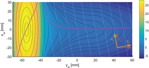
The benefit of the contact locus is that it reduces the contact search to a one-dimensional problem. Other ways to achieve the same were presented by different authors [45,76,77]. Wang's method was extended further to wheel-on-rollers [72,78]. Involved analyses are used in all of these cases. Here we present a new derivation for the contact locus for wheel-on-rail configurations that's easier to understand, and present its extension to wheel-on-roller contacts.

4.1. Contact locus for wheel-on-rail contact

For wheel-on-rail contact, we consider a prismatic rail, where the surface height $z_{rail(r)}$ is a function of lateral position only, $z_{rail(r)}(x_{(r)},y_{(r)})=h_{rail}(y_{(r)})$. This makes for a surface that's horizontal in the longitudinal directions of the rail and track systems. A necessary condition for the gap $g=z_{rail(r)}-z_{wh(r)}$ to be locally minimum is then that the wheel be horizontal also, when viewed along lines of constant $y_{(r)}$. (32) $\frac{\mathrm{\partial }{z}_{wh(r)}}{\mathrm{\partial }{x}_{(r)}}=0.$(32) This is illustrated in Figure 11, for a wheel with new S1002 profile, with a nominal radius $r_{nom,w}=120\text{mm}$ to exaggerate the surface variation, showing the profile height $z_{wh(w)}$ in the wheel profile system. Light-blue lines indicate the orientation of the rail forward direction, $x_{(r)}$, for a yaw angle ${\psi }_{ws}={10}^{\circ }$. Black curves indicate the contour lines of constant surface height. The contact locus of equation (32(32) $\frac{\mathrm{\partial }{z}_{wh(r)}}{\mathrm{\partial }{x}_{(r)}}=0.$(32) ) is then obtained as the points where the contours touch on the light-blue lines of constant $y_{(r)}$, as shown by the magenta curve.

The directional derivative $\mathrm{\partial }{z}_{wh(w)}/\mathrm{\partial }{x}_{(r)}$, along the light-blue lines, is obtained multiplying the gradient with the desired direction vector $\mathbf{t}=[\cos (\psi ),-\sin (\psi ){]}^T$. This brings condition (32(32) $\frac{\mathrm{\partial }{z}_{wh(r)}}{\mathrm{\partial }{x}_{(r)}}=0.$(32) ) for a horizontal tangent to (33) $\cos (\psi )\frac{\mathrm{\partial }{z}_{wh(w)}}{\mathrm{\partial }{x}_{(w)}}-\sin (\psi )\frac{\mathrm{\partial }{z}_{wh(w)}}{\mathrm{\partial }{y}_{(w)}}=0.$(33) These principles, illustrated in Figure 11, are formalised using appropriate mathematics notations. The wheel surface is defined implicitly in wheel coordinates as the set of points satisfying the equation (34) $x_{wh(w)}^2+(z_{wh(w)}-z_{mid,w}{)}^2=(r_{wh}(y_{wh(w)}){)}^2,z_{mid,w}=-r_{nom,w}.$(34) This is embedded in 3D space using the level set $f_{wh(w)}({\mathbf{x}}_{(w)})=0$, using a function $f_{wh(w)}$: (35) $\begin{array}{rl}& f_{wh(w)}:{\mathbb{R}}_{(w)}^3\to \mathbb{R},\\ & f_{wh(w)}(x_{(w)},y_{(w)},z_{(w)})=x_{(w)}^2+(z_{(w)}-z_{mid,w}{)}^2-(r_{wh}(y_{(w)}){)}^2.\end{array}$(35) Here $r_{wh}=r_{nom,w}+h_{wh}(y_{(w)})$ is the radius of a circle at $y_{(w)}$, centred at $x_{(w)}=0,z_{(w)}=z_{mid,w}$. The function $f_{wh(w)}$, containing the wheel surface, is transformed to rail coordinates by successive rotations. The transformation is written as ${\mathbf{x}}_{(w)}={\mathbf{x}}_{(w)}({\mathbf{x}}_{(r)})$: (36) $\begin{array}{rl}& {\mathbf{x}}_{(w)}:{\mathbb{R}}_{(r)}^3\to {\mathbb{R}}_{(w)}^3,{\mathbf{x}}_{(w)}={\mathbf{o}}_{(w)}^{rail}+{\mathbf{R}}_{(w)}^{rail}{\mathbf{x}}_{(r)},\\ & f_{wh(r)}:{\mathbb{R}}_{(r)}^3\to \mathbb{R},f_{wh(r)}=f_{wh(w)}\circ {\mathbf{x}}_{(w)},\text{i.e.}{f}_{wh(r)}({\mathbf{x}}_{(r)})=f_{wh(w)}({\mathbf{x}}_{(w)}({\mathbf{x}}_{(r)})).\end{array}$(36) The rotation matrix from rail to wheel coordinates is obtained using the rotation from rail to track coordinates times the inverse from wheel to track coordinates. Using Equation (4(4) $\begin{array}{r}\mathbf{R}(\varphi \text{--}\psi )=\left[\begin{array}{ccc}1& 0& 0\\ 0& c_{\varphi }& -s_{\varphi }\\ 0& s_{\varphi }& c_{\varphi }\end{array}\right]\left[\begin{array}{ccc}{c}_{\psi }& -s_{\psi }& 0\\ s_{\psi }& c_{\psi }& 0\\ 0& 0& 1\end{array}\right]=\left[\begin{array}{ccc}{c}_{\psi }& -s_{\psi }& 0\\ c_{\varphi }{s}_{\psi }& c_{\varphi }{c}_{\psi }& -s_{\varphi }\\ s_{\varphi }{s}_{\psi }& s_{\varphi }{c}_{\psi }& c_{\varphi }\end{array}\right].\end{array}$(4) ), for the roll–yaw–pitch convention: (37) ${\mathbf{R}}_{(w)}^{rail}=\mathbf{R}(\varphi \text{--}\psi {)}^T=\left[\begin{array}{ccc}{c}_{\psi }& c_{\varphi }{s}_{\psi }& s_{\varphi }{s}_{\psi }\\ -s_{\psi }& c_{\varphi }{c}_{\psi }& s_{\varphi }{c}_{\psi }\\ 0& -s_{\varphi }& c_{\varphi }\end{array}\right]$(37) In this case, the angle ϕ may contain roll of the wheelset as well as the cant of the rail.

The wheel surface is extracted from the function $f_{wh(r)}$ in rail coordinates using the implicit function theorem. This says that there exists an explicit function $z_{wh(r)}$ corresponding to the surface $f_{wh(r)}=0$, except for places with vanishing derivative $\mathrm{\partial }{f}_{wh(r)}/\mathrm{\partial }{z}_{(r)}=0$: (38) $z_{wh(r)}:{\mathbb{R}}_{(r)}^2\to \mathbb{R},z_{wh(r)}=z_{wh(r)}(x_{(r)},y_{(r)}).$(38) The partial derivatives of $z_{wh(r)}$ are obtained through implicit differentiation of the level $f_{wh(r)}=0$ with respect to $x_{(r)}$: (39) $\frac{\mathrm{\partial }{f}_{wh(r)}}{\mathrm{\partial }{x}_{(r)}}+\frac{\mathrm{\partial }{f}_{wh(r)}}{\mathrm{\partial }{z}_{(r)}}\frac{\mathrm{\partial }{z}_{wh(r)}}{\mathrm{\partial }{x}_{(r)}}=0\to \frac{\mathrm{\partial }{z}_{wh(r)}}{\mathrm{\partial }{x}_{(r)}}=-\frac{\mathrm{\partial }{f}_{wh(r)}}{\mathrm{\partial }{x}_{(r)}}/\frac{\mathrm{\partial }{f}_{wh(r)}}{\mathrm{\partial }{z}_{(r)}}.$(39) Next, we obtain the partial derivatives of $f_{wh(r)}$ using the chain rule and the gradient of $f_{wh(w)}$: (40a) $\begin{array}{rl}\mathrm{\nabla }{f}_{wh(w)}({\mathbf{x}}_{(w)})& =[2x_{(w)},-2r_{wh}(y_{(w)})h_{wh}^{\prime }(y_{(w)}),2(z_{(w)}-z_{mid,w})],\end{array}$(40a) (40b) $\begin{array}{rl}\mathrm{\nabla }{f}_{wh(r)}({\mathbf{x}}_{(r)})& =\mathrm{\nabla }{f}_{wh(w)}({\mathbf{x}}_{(w)}({\mathbf{x}}_{(r)}))\cdot {\mathbf{R}}_{(w)}^{rail}.\end{array}$(40b) The contact locus on the wheel follows as (41) $\begin{array}{rl}\frac{\mathrm{\partial }{z}_{wh(r)}}{\mathrm{\partial }{x}_{(r)}}\stackrel{?}{=}0& \to \frac{\mathrm{\partial }{f}_{wh(r)}}{\mathrm{\partial }{x}_{(r)}}=2x_{(w)}\cdot c_{\psi }-2r_{wh}(y_{(w)})h_{wh}^{\prime }(y_{(w)})\cdot -s_{\psi }\stackrel{?}{=}0\\ & \to x_{lc(w)}=-r_{wh}(y_{(w)})h_{wh}^{\prime }(y_{(w)})\tan (\psi ).\end{array}$(41) The derivative $h_{wh}^{\prime }$ takes h as a function of $y_{wh}$, whereas the profile points may be given with $y_{wh}$ decreasing. This requires a bit of care to get the right sign. Computations for the left wheel are done with mirroring, using right-sided profiles, such that the derivative $h^{\prime }$ isn't affected. Note that mirroring changes the sign of ${\psi }_{ws}$.

The contact locus on the wheel is transformed to track coordinates and used to form the gap function. All local minima are determined and used to define contact patches. The lateral extent follows from the range where negative gap values are found. In longitudinal direction, the length of interpenetration areas is estimated using the maximum penetration ${\delta }_n$ and the effective radius $r_{eff}=r(y_w)/\cos ({\delta }_{cp(tr)})$ [26], using a quadratic approximation.

The reason why our formula looks so much easier than Wang's contact locus resides in the use of the roll–yaw–pitch convention. A different matrix shows up when starting from the yaw–roll–pitch convention, (42) ${\mathbf{R}}_{yaw(w)}^{rail}=\mathbf{R}(\psi \text{--}\varphi {)}^T=\left[\begin{array}{ccc}{c}_{\psi }& s_{\psi }& 0\\ -s_{\psi }{c}_{\varphi }& c_{\psi }{c}_{\varphi }& s_{\varphi }\\ s_{\psi }{s}_{\varphi }& -c_{\psi }{s}_{\varphi }& c_{\varphi }\end{array}\right].$(42) The first column multiplied with the gradient $\mathrm{\nabla }{f}_{wh(w)}$ of Equation (40a(40a) $\begin{array}{rl}\mathrm{\nabla }{f}_{wh(w)}({\mathbf{x}}_{(w)})& =[2x_{(w)},-2r_{wh}(y_{(w)})h_{wh}^{\prime }(y_{(w)}),2(z_{(w)}-z_{mid,w})],\end{array}$(40a) ) gives: (43) $\frac{\mathrm{\partial }{f}_{wh(r)}}{\mathrm{\partial }{x}_{(r)}}=2x_{(w)}\cdot c_{\psi }-2r_{wh}(y_{(w)})h_{wh}^{\prime }(y_{(w)})\cdot -s_{\psi }{c}_{\varphi }+2(z_{(w)}-z_{mid,w})\cdot s_{\psi }{s}_{\varphi }\stackrel{?}{=}0$(43) This reduces to (41(41) $\begin{array}{rl}\frac{\mathrm{\partial }{z}_{wh(r)}}{\mathrm{\partial }{x}_{(r)}}\stackrel{?}{=}0& \to \frac{\mathrm{\partial }{f}_{wh(r)}}{\mathrm{\partial }{x}_{(r)}}=2x_{(w)}\cdot c_{\psi }-2r_{wh}(y_{(w)})h_{wh}^{\prime }(y_{(w)})\cdot -s_{\psi }\stackrel{?}{=}0\\ & \to x_{lc(w)}=-r_{wh}(y_{(w)})h_{wh}^{\prime }(y_{(w)})\tan (\psi ).\end{array}$(41) ) when $\varphi =0$, dropping the $z_{(w)}$ contribution, but cannot be inverted so easily when $z_{(w)}$ is retained. The detailed formulas were given by Wang [32]. Equation (41(41) $\begin{array}{rl}\frac{\mathrm{\partial }{z}_{wh(r)}}{\mathrm{\partial }{x}_{(r)}}\stackrel{?}{=}0& \to \frac{\mathrm{\partial }{f}_{wh(r)}}{\mathrm{\partial }{x}_{(r)}}=2x_{(w)}\cdot c_{\psi }-2r_{wh}(y_{(w)})h_{wh}^{\prime }(y_{(w)})\cdot -s_{\psi }\stackrel{?}{=}0\\ & \to x_{lc(w)}=-r_{wh}(y_{(w)})h_{wh}^{\prime }(y_{(w)})\tan (\psi ).\end{array}$(41) ) can be used as an easy and satisfactory approximation. In this case, the roll angle ϕ should consider the wheelset roll only. Rail cant doesn't affect the contact locus for wheel/rail contact.

4.2. Contact locus for a wheel on a roller

Our approach for a wheel on a roller works along the same lines, even though it looks more complicated. The starting point is that a locally minimum value of the gap function requires equal slopes of the surfaces of wheel and roller: (44) $\frac{\mathrm{\partial }{z}_{wh(r)}}{\mathrm{\partial }{x}_{(r)}}=\frac{\mathrm{\partial }{z}_{rol(r)}}{\mathrm{\partial }{x}_{(r)}}.$(44) The slope of the roller surface is developed similarly as the slope on the wheel surface above, except that no coordinate rotation is needed in this case: (45a) $\begin{array}{rl}& f_{rol(r)}:{\mathbb{R}}_{(r)}^3\to \mathbb{R},\\ & f_{rol(r)}(x_{(r)},y_{(r)},z_{(r)})=x_{(r)}^2+(z_{(r)}-z_{mid,r}{)}^2-(r_{rol}(y_{(r)}){)}^2,\end{array}$(45a) (45b) $\begin{array}{rl}& \mathrm{\nabla }{f}_{rol(r)}({\mathbf{x}}_{(r)})=[2x_{(r)},2r_{rol}(y_{(r)})h_{rol}^{\prime }(y_{(r)}),2(z_{(r)}-z_{mid,r})].\end{array}$(45b) Here $r_{rol}=r_{nom,r}-h_{rol}(y_{(r)})$ is the radius of a circle at $y_{(r)}$, centred at $x_{(r)}=0,z_{(r)}=z_{mid,r}=r_{nom,r}$. A function $z_{rol(r)}$ exists to describe the roller's surface: (46) $z_{rol(r)}:{\mathbb{R}}_{(r)}^2\to \mathbb{R},z_{rol(r)}=z_{rol(r)}(x_{(r)},y_{(r)}).$(46) The derivative in $x_{(r)}$-direction is obtained as: (47) $\frac{\mathrm{\partial }{z}_{rol(r)}}{\mathrm{\partial }{x}_{(r)}}=-\frac{\mathrm{\partial }{f}_{rol(r)}}{\mathrm{\partial }{x}_{(r)}}/\frac{\mathrm{\partial }{f}_{rol(r)}}{\mathrm{\partial }{z}_{(r)}}=-\frac{x_{(r)}}{z_{(r)}-r_{nom,r}}.$(47) The denominator of (39(39) $\frac{\mathrm{\partial }{f}_{wh(r)}}{\mathrm{\partial }{x}_{(r)}}+\frac{\mathrm{\partial }{f}_{wh(r)}}{\mathrm{\partial }{z}_{(r)}}\frac{\mathrm{\partial }{z}_{wh(r)}}{\mathrm{\partial }{x}_{(r)}}=0\to \frac{\mathrm{\partial }{z}_{wh(r)}}{\mathrm{\partial }{x}_{(r)}}=-\frac{\mathrm{\partial }{f}_{wh(r)}}{\mathrm{\partial }{x}_{(r)}}/\frac{\mathrm{\partial }{f}_{wh(r)}}{\mathrm{\partial }{z}_{(r)}}.$(39) ) must now be expanded, which could be ignored in the case of a wheel on a rail. (48) $\frac{\mathrm{\partial }{f}_{wh(r)}}{\mathrm{\partial }{z}_{(r)}}=2x_{(w)}{s}_{\varphi }{s}_{\psi }-2r_{wh}(y_{(w)})h_{wh}^{\prime }(y_{(w)})s_{\varphi }{c}_{\psi }+2(z_{(w)}+r_{nom,w})c_{\varphi }.$(48) The contact locus on the wheel follows as (49) $-\frac{x_{(w)}{c}_{\psi }+r_{wh}(y_{(w)})h_{wh}^{\prime }(y_{(w)})s_{\psi }}{x_{(w)}{s}_{\varphi }{s}_{\psi }-r_{wh}(y_{(w)})h_{wh}^{\prime }(y_{(w)})s_{\varphi }{c}_{\psi }+(z_{(w)}+r_{nom,w})c_{\varphi }}\stackrel{?}{=}-\frac{x_{(r)}}{z_{(r)}-r_{nom,r}}.$(49) This is solved quickly using an iterative procedure, for each position $y_w$ where the locus is desired: (50) $\frac{x_{(w)}^{k+1}{c}_{\psi }+r_{wh}(y_{(w)})h_{wh}^{\prime }(y_{(w)})s_{\psi }}{x_{(w)}^k{s}_{\varphi }{s}_{\psi }-r_{wh}(y_{(w)})h_{wh}^{\prime }(y_{(w)})s_{\varphi }{c}_{\psi }+(z_{(w)}^k+r_{nom,w})c_{\varphi }}=\frac{x_{(r)}^k+x_{(w)}^{k+1}-x_{(w)}^k}{z_{(r)}^k-r_{nom,r}}.$(50) This converges in two steps even when starting from $x_{(w)}^0=0$.

When using mirroring of the left side to a right side problem, ${\varphi }_{ws}$ and ${\psi }_{ws}$ are both affected. The resulting method is cross-validated using the brute-force approach.

5. Results

The main capability of the method presented is to analyse wheel/rail contacts using a 3-d contact search algorithm. Some typical examples will be shown for this using the Manchester contact benchmark [13,79]. Further results are shown for a collection of measured worn profiles, demonstrating the automation and robustness of the calculations.

5.1. Results for the Manchester contact benchmark

The Manchester contact benchmark was proposed to assess the impact of wheel-rail contact modelling assumptions on the simulation of railway vehicle dynamics [13,79]. Two simulation cases were considered initially: case A for a single wheelset, to consider contact methods in isolation, and case B for a railway vehicle, to assess the effect of contact methods on vehicle dynamics. The paper [13] presents the results for case A for ten codes that participated. The work seems to have stopped thereafter, with no results published yet for case B.

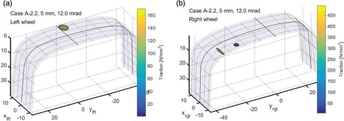
Here we focus attention on test-case A-2.2 for the tangential contact problem, for a wheelset with new S1002 and UIC60 wheel and rail profiles with lateral displacement and yaw angles increasing in proportion to each other. Figure 12 shows results for one such position, $y_{ws}=5\text{mm},{\psi }_{ws}=12.0\text{mrad}$, where two contact patches are found on the right rail. Thick lines on the rail profile indicate the curves $x_{(r)}=0$ and $y_{(r)}=0$, with the origin of the rail coordinate system at the crossing of these curves. As the wheelset steers to the right at a positive yaw angle, contact is found on the left rail at positive $x_{(r)}$, and at $x_{(r)}<0$ on the right rail. These x-locations are a direct output of the 3-d contact search algorithm.

Figure 12. Wheel/rail contact results for the Manchester benchmark test-case A-2.2: wheelset with lateral displacement $y_{ws}=5\text{mm}$, yawed at ${\psi }_{ws}=12.0\text{mrad}$.

A particularly challenging configuration was identified by Kienberger for the contact of the wheel flange root to the rail gauge corner [38], leading to strongly non-elliptic contact as illustrated in Figure 13 (left). This concerns case A-2.2 of the Manchester benchmark computed using the Kalker CONTACT add-on to SIMPACK Rail, at lateral shift $y_{ws}=6.5\text{mm}$, yaw angle ${\psi }_{ws}=15.6\text{mrad}$, and a vertical force $F_z=80\text{kN}$ per wheel. Similar shapes were presented by Baeza et al. [40], at $y_{ws}=6.3\text{mm},{\psi }_{ws}=17.5\text{mrad}$. Figures 13, middle and right, show the corresponding result obtained from CONTACT, at $y_{ws}=4.954\text{mm},{\psi }_{ws}=15.6\text{mrad}$. This shows that good agreement is reached at slightly shifted locations. The discrepancy comes from the different conventions used: measuring the lateral shift at the height of the axle or in the track plane. Further, the contact patch appears shifted by $(\pm 2,\pm 1\text{mm})$ in the local coordinate system. This comes from using slightly different weighting in the calculation of the contact reference position.

Figure 13. Left: results obtained using the Kalker CONTACT add-on to SIMPACK rail [38]. Middle, right: corresponding results for the new w/r geometry module.

The contact positions reported by CONTACT concern the weighted reference cf. Equation (12(12) $[x_{tr},y_{tr},{\alpha }_{tr}{]}_{cwgt2}={\int }_{g<0}[x,y,\alpha ]g^2(x,y)\text{d}x\text{d}y/{\int }_{g<0}{g}^2(x,y)\text{d}x\text{d}y.$(12) ). These are shown in Figure 14, plotted on top of the results published for the Manchester benchmark. In overall sense, the results show good correspondence. Somewhat bigger differences occur around the centred position, $y_{ws}\le 0.5\text{mm}$, that yields wide, asymmetric contact patches. These differences do not much affect the computed forces, or the integration in a vehicle dynamics simulation, as long as creepages, contact location and force location are used in a consistent way. This is considered in more detail in the accompanying paper [44].

Figure 14. Lateral contact positions on the rail for Manchester contact benchmark case A1.1 new profiles $20\text{kN}$ load, computed by CONTACT, plotted on top of benchmark results presented by Shackleton and Iwnicki [13, Figure 3].

The Manchester benchmark concerns a free rolling wheelset, including an equilibrium equation $\sum M_{y(ws)}=0$ for the net moment on the wheelset in its rolling direction, and a similar balance to distribute the load over the wheels. Focusing on a single wheel and rail, these are not included in CONTACT. Instead, a small iteration procedure is programmed in Matlab that tunes the wheelset vertical position, roll angle, and pitch velocity, to satisfy the balance equations. Figures 15 and 16 show the longitudinal and lateral contact forces computed by CONTACT, plotted on top of the published results. The brute-force method and the contact locus produce identical values, except for minimal effects of the discretisation. These new results are generally in good agreement with the earlier ones.

Figure 15. Longitudinal contact forces for Manchester contact benchmark case A2.2 new profiles $20\text{kN}$ load, computed by CONTACT, plotted on top of benchmark results presented by Shackleton and Iwnicki [13, Figure 16].

Figure 16. Lateral contact forces for Manchester contact benchmark case A2.2 new profiles $20\text{kN}$ load, computed by CONTACT, plotted on top of benchmark results presented by Shackleton and Iwnicki [13, Figure 17].

5.2. Results for a thousand freight cars with worn profiles

A further application that's considered here concerns a project on rail life extension performed for CSX, a North American class I railroad. A simulation approach is developed to assess rail profile evolution considering wear and grinding. This work is performed by Sentient Science, NRC Canada, and Vtech CMCC, using VAMPIRE and the CONTACT software.

The target for a simulation is to evaluate the life of rails at one segment of track for a given operational scenario. An example considered in the project concerns a $5^{\circ }$ curve, radius $349\text{m}$, near Cartersville, GA. Traffic data are collected for the segment: the number of trains, types of wagons, loads, speeds, wheel profiles, as well as track data, e.g. geometry, friction management practices. These data are analysed and classified, e.g. distinguishing different quality levels [80]. Loading ensembles are then defined that represent the actual situation, maintaining the ranges and variability of input parameters, however, with a much reduced number of loadings. Simulations with VAMPIRE are used to assess the vehicle dynamics in steady curving, using VAMPIRE's internal contact algorithms. The contact situation is then analysed in detail using CONTACT, using the wheelset kinematics as obtained from VAMPIRE, maintaining the vertical force $F_{z(tr)}$ that governs the level of the contact stresses. These stresses are then fed into Sentient's wear and grinding calculations. This is repeated multiple times, until the rail profile is worn down to a predefined threshold and the life is exhausted.

The challenge for CONTACT in this application lies in the robust and automatic calculation of a wide range of contact situations. This is demonstrated considering the so-called ‘group 5 data’, the 20% of wheels with the lowest profile quality index. A thousand freight cars are simulated, a mixture of flat, hopper and tank cars. Speeds vary between 7 and $40\text{mph}$ (11–64 km/h), and weights between 50,000 and 300,000 lbs (222–1334 kN) for empty and full wagons. Two axles are considered for each car, for the leading bogie. Four coefficients of friction are set for each axle, two for each wheel, taken from normal distributions with mean $\overline{\mu }=0.35$ and standard deviation ${\sigma }_{\mu }=0.16$ at the top of the rail (surface inclination $\alpha \le {20}^{\circ }$) and $\overline{\mu }=0.20,{\sigma }_{\mu }=0.0167$ at the gauge face ($\alpha \ge {30}^{\circ }$). All wheels encountered in this collection are heavily worn, while some profiles have missing data: gaps, or ending prematurely.

This test-set of four thousand wheels appeared to present scenarios that had not yet been encountered. Additional work was needed to detect and handle all edge cases appropriately. For instance for the arc length along the profiles, used in the parametric spline representation, it appears tricky sometimes to define the reference s = 0 at the profile reference marker. This happened particularly for wheels where the wheel marker lies at the back of the flange, with multiple crossings of the profile with the abcissa $y_w=0$. Another example concerns the contact locus with $x_{lc}$ tending to infinity at vertical slopes in the profile. Next, the computation of the weighted centre (Equation (12(12) $[x_{tr},y_{tr},{\alpha }_{tr}{]}_{cwgt2}={\int }_{g<0}[x,y,\alpha ]g^2(x,y)\text{d}x\text{d}y/{\int }_{g<0}{g}^2(x,y)\text{d}x\text{d}y.$(12) )), must be prepared for cases with only minimal interpenetration (e.g. $\mathcal{O}({10}^{-9})$). Such cases aren't relevant from a practical perspective, still, the programme should take care not to divide by zero.

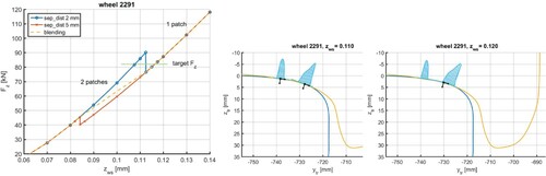
Figure 17 shows a situation where the combination of contact patches is activated. Initially, using a combination distance $d_{comb}=d_{sep}=2\text{mm}$, combination of patches occurs at vertical positions $z_{ws}\ge 0.1125$. The computed vertical force then jumps from 90 to $76\text{kN}$, hampering convergence for a solution procedure that tries to solve $z_{ws}$ for $F_z=82\text{kN}$. This may be resolved using $d_{comb}=d_{sep}=5\text{mm}$, but that merely moves the trouble to other cases. A more durable resolution is provided by the blending approach, smoothing the function $F_z=F_z(z_{ws})$. The solution algorithm used for this balance equation is also extended such that it proceeds with sensible values when a jump is encountered.

Figure 17. Combination of contact patches for wheel 2291. The vertical force jumps suddenly at increasing vertical positions when using a single threshold, and changes gradually when using the blending approach.

Further issues are related to profile smoothing. We currently don't have good guidelines for the parameter λ of Equation (10(10) $L=\sum _{i=1}^n{\left(\frac{y_i-Y(s_i)}{{\sigma }_i}\right)}^2+\lambda {\int }_{s_1}^{s_n}{(Y^{″}(s))}^2\text{d}s$(10) ). This depends on the spacing of the profile points and on the inherent curvature contained in the profile. λ is currently tuned by trial and error, on the basis of Figure 18 for instance. Parameters $\lambda =0.1\text{--}1$ could be used for these profiles if there's good confidence in the measured values and if one is interested in the effects of pressure variations. Bigger values like $\lambda =5\text{--}10$ could be appropriate if one is interested more in the general behaviour.

Figure 18. Computed pressures $p_n$ for one case of the group 5 data with varying levels of profile smoothing.

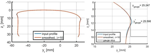
Smoothing appears to have subtle interactions with the positioning of wheel and rail profiles. This occurs when certain characteristics of profiles are used to put them in place, like raising or lowering the rail to touch the track plane precisely. Another case where this occurs is in the gauge point computation. This is shown in Figure 19 for a rail that bulges out due to plastic deformation. Using $\lambda =10$, reduces the bump by $0.24\text{mm}$, shifting the whole profile by the same amount. These are quite large displacements considering the strong sensitivity of contact problems to the amount of indentation. As a result, position values should be treated with care, with an eye on the context in which they were computed, and should usually be obtained using additional balance equations.

Figure 19. Strong profile smoothing ($\lambda =10$) changes the gauge point by $0.24\text{mm}$ on this profile with localised features.

6. Conclusions and discussion

This paper presented the computational methods and software design for the new module for wheel/rail contact geometry analysis that is implemented in CONTACT. Building on many components developed by others, this module automates and greatly simplifies the running of CONTACT for generic wheel/rail contact situations. Fully 3-d contact search algorithms are implemented. This uses the contact locus approach, that's simplified for wheel-on-rail situations and extended to wheel-on-roller contacts.

A main characteristic of the new module is its extensive use of the multibody formalism, using markers to represent coordinate systems, and the design using a generic, object oriented-like software foundation. This simplifies the development of new algorithms. We no longer have to analyse the 3-d contact geometry using pen and paper, making transformations ourselves, yet can build the geometry in one coordinate system and transform to another. This complements analytical approaches that provide more insight but are more difficult to develop and generalise. 1-d parametric spline curves and bi-linear interpolation are used and give satisfactory results; 2-d spline surfaces could provide additional flexibility with respect to the needed operations.

The contact geometry is analysed twice; first for the location of contact patches, and then for the local geometry of the contact patches. The contact search works in overall vertical direction and starts from the wheel and rail profiles in ther actual, overlapping positions. Besides the contact location, defined using weighted averaging, this identifies the extent of interpenetration areas also. Potential contact areas are defined accordingly, discretised, and used to compute the undeformed distance in normal direction. Creepages are formed automatically using rigid body kinematics, including wheel and track flexible bending. This again complements analytical approximations, allowing for cross-validation.

Numerical results illustrate the viability, generality, and robustness of the approach, dealing with strongly asymmetric contact patches and situations where multiple contact patches occur. Results are shown for the Manchester contact benchmark that correspond well to the published results. Further results concern a collection of heavily worn wheel profiles, illustrating the level of automation of the approach. The different strategies used in the planar contact approach, for the contact reference point and the reference angle, are discussed in a separate paper [44].

A challenge for the planar contact approach comes from the combination of nearby contact patches. This is desired to account for their interaction but unwanted because of the compromise introduced for the contact reference angle. To strike a balance between these different wishes, a criterion is introduced on the basis of the distance between adjacent patches. However, such switches may cause discontinuities in the numerical results at slight perturbations of input parameters, such as a prescribed vertical force. This hampers the integration in multi-body dynamics simulation, or the solution of additional balance equations. A blending approach is introduced to mitigate some of the jumps, more research is needed to reduce the jumps further.

Further work is needed on the extension of the approach to more general geometrical configurations. For instance, the overall vertical direction may not be appropriate in the computation of contacts with a check rail. This may be addressed using a prior analysis to find a reasonably ‘normal’ orientation. In rolling direction, geometrical deviations are introduced by wheel flats, out-of-roundness, and corrugation. It's unclear whether the contact locus approach can be extended for this. Otherwise, the grid-based approach should be improved with respect to its performance. Finally, short wavelength variations in rolling direction may call for transient instead of steady rolling computations, addressing fluctuations in the creepage and creep forces. This calls for connecting the grids and contact patches between consecutive time steps, and for further integration of the contact calculations in multi-body dynamics simulation.

Acknowledgments

Thanks to many colleagues for valuable discussions that contributed to this work indirectly. Thanks to Julio Blanco Lorenzo, Javier Santamaria, and Ernesto Garcia Vadillo for their direct contributions and reviewing the draft version of this paper. Thanks to CSX (Dan Hampton) for permitting use of the test-cases discussed in Section 5.2, and thanks to the colleagues at LORAM, NRC and Sentient Science that contributed to the collection and preparation of these data. Thanks finally to the anonymous reviewers for their valuable feedback on this paper.

Disclosure statement

No potential conflict of interest was reported by the author(s).

References

- Iwnicki S, editor. Proceedings of the 22nd International Symposium on Dynamics of Vehicles on Roads and Tracks. Manchester: IAVSD; 2011.
- Rosenberger M, editor. Proceedings of the 24th International Symposium on Dynamics of Vehicles on Roads and Tracks. Graz, Austria: IAVSD; 2015.
- Spiryagin M, Gordon T, Cole C, et al., editor. Proceedings of the 25th International Symposium on Dynamics of Vehicles on Roads and Tracks. Rockhampton, Queensland, Australia: IAVSD; 2017.
- Lunden R, Ekberg A, Berg M, et al. Special edition of “Wear” to contain CM2015 proceedings. Wear. 2016;366–367:1–2.
- Li Z, Núñez A, editors. Proceedings of the 11th International Conference on Contact Mechanics and Wear of Rail/Wheel Systems. The Netherlands: Delft University of Technology; 2018.
- Meymand S, Keylin A, Ahmadian M. A survey of wheel-rail contact models for rail vehicles. Veh Syst Dyn. 2016;54:386–428.
- Zhai W, Han Z, Chen Z, et al. Train-track-bridge dynamic interaction: a state-of-the-art review. Veh Syst Dyn. 2019;57:984–1027.
- Kalker J. The computation of three-dimensional rolling contact with dry friction. Int J Numer Methods Eng. 1979;14:1293–1307.
- Kalker J. Two algorithms for the contact problem in elastostatics. Delft (The Netherlands): Delft University of Technology, report TWI 82-26; 1982.
- Kalker J. Numerical calculation of the elastic field in a half-space. Comm Appl Num Meth. 1986;2:401–410. Reprinted as Appendix C in Kalker J. Three-dimensional elastic bodies in rolling contact. Dordrecht: Kluwer Academic Publishers; 1990. (Solid mechanics and its applications; vol. 2).
- Kalker J. Mathematical models of friction for contact problems in elasticity. Wear. 1986;113:61–77.
- Kalker J. Three-dimensional elastic bodies in rolling contact. Dordrecht: Kluwer Academic Publishers; 1990. (Solid mechanics and its applications; vol. 2).
- Shackleton P, Iwnicki S. Comparison of wheel-rail contact codes for railway vehicle simulation: an introduction to the Manchester Contact Benchmark and initial results. Veh Syst Dyn. 2008;46(1–2):129–149.
- Baeza L, Vila P, Roda A, et al. Prediction of corrugation in rails using a non-stationary contact model. Wear. 2008;265:1156–1162.
- Willner K. Fully coupled frictional contact using elastic halfspace theory. ASME J Tribol. 2008;130:031405-1–031405-8.
- Pieringer A, Kropp W, Thompson D. Investigation of the dynamic contact filter effect in vertical wheel/rail interaction using a 2D and a 3D non-Hertzian contact model. Wear. 2011;271(1–2):328–338.
- Kaiser I. Refining the modelling of vehicle-track interaction. In: Iwnicki S, editor. Proceedings of the 22nd International Symposium on Dynamics of Vehicles on Roads and Tracks. Manchester: IAVSD; 2011. p. 1–6.
- Blanco-Lorenzo J, Santamaria J, Vadillo E, et al. On the influence of conformity on wheel-rail rolling contact mechanics. Tribol Int. 2016;103:647–667.
- Vollebregt E. Improving the speed and accuracy of the frictional rolling contact model “CONTACT”. In: Topping B, Adam J, Pallarés F, et al., editors. Proceedings of the 10th International Conference on Computational Structures Technology; Stirlingshire, United Kingdom. Civil-Comp Press; 2010. p. 1–15. DOI:https://doi.org/10.4203/ccp.93.17.
- Vollebregt E. A new solver for the elastic normal contact problem using conjugate gradients, deflation, and an FFT-based preconditioner. J Comput Phys. 2014;257, Part A:333–351.
- Zhao J, Vollebregt E, Oosterlee C. A fast nonlinear conjugate gradient based method for 3D concentrated frictional contact problems. J Comput Phys. 2015;288:86–100.
- Vollebregt E. Numerical modeling of measured railway creep versus creep-force curves with CONTACT. Wear. 2014;314:87–95.
- Wekken Cvd, Vollebregt E. Local plasticity modelling and its influence on wheel-rail friction. In: Li Z, Núñez A, editors. Proceedings of the 11th International Conference on Contact Mechanics and Wear of Rail/Wheel Systems. The Netherlands: Delft University of Technology; 2018. p. 1013–1018.
- Vollebregt E, van der Wekken C. Advanced modeling of wheel-rail friction phenomena. VORtech; 2019. TR19-11. FRA project.
- Vollebregt E, Segal A. Solving conformal wheel-rail rolling contact problems. Veh Syst Dyn. 2014;52(suppl. 1):455–468. DOI:https://doi.org/10.1080/00423114.2014.906634
- Vollebregt E. Conformal contact: corrections and new results. Veh Syst Dyn. 2018;56(10):1622–1632. DOI:https://doi.org/10.1080/00423114.2018.1424917
- Vollebregt E. User guide for CONTACT, Rolling and sliding contact with friction. Vtech CMCC; 2020. TR20-01, version 20.2. Available from: www.cmcc.nl/documentation.
- Pater Ad. The geometrical contact between track and wheelset. Veh Syst Dyn. 1988;17(3):127–140.
- Shabana A, Zaazaa K, Escalona J, et al. Development of elastic force model for wheel/rail contact problems. J Sound Vib. 2004;269:295–325.
- Pombo J, Ambrósio J, Silva M. A new wheel-rail contact model for railway dynamics. Veh Syst Dyn. 2007;45:165–189.
- Shabana A, Zaazaa K, Sugiyama H. Railroad vehicle dynamics: a computational approach. Boca Raton: CRC Press; 2008.
- Wang K. The track of wheel contact points and the calculation of wheel/rail geometric contact parameters. J Southwest Jiaotong Univ. 1984;1:89–99.
- Li Z. Wheel-rail rolling contact and its application to wear simulation [dissertation]. Delft University of Technology; 2002.
- Jin X, Wen Z, Zhang W, et al. Numerical simulation of rail corrugation on a curved track. Comput Struct. 2005;83:2052–2065.
- Santamaría J, Vadillo E, Gómez J. A comprehensive method for the elastic calculation of the two-point wheel-rail contact. Veh Syst Dyn. 2006;44, suppl:240–250.
- Malvezzi M, Meli E, Falomi S, et al. Determination of wheel-rail contact points with semianalytic methods. Multibody Syst Dyn. 2008;20:327–358.
- Sugiyama H, Suda Y. On the contact search algorithms for wheel/rail contact problems. J Comput Nonlinear Dyn Trans ASME. 2009;4:041001.
- Vollebregt E, Weidemann C, Kienberger A. Use of “CONTACT” in multi-body vehicle dynamics and profile wear simulation: initial results. In: Iwnicki S, editor. Proceedings of the 22nd International Symposium on Dynamics of Vehicles on Roads and Tracks. Manchester: IAVSD; 2011. p. 1–6.
- Yang X, Gu S, Zhou S, et al. A method for improved accuracy in three dimensions for determining wheel/rail contact points. Veh Syst Dyn. 2015;53:1620–1640.
- Baeza L, Thompson D, Squicciarini G, et al. Method for obtaining the wheel-rail contact location and its application to the normal problem calculation through “CONTACT”. Veh Syst Dyn. 2018;56:1734–1746.
- An B, Wen J, Wang P, et al. Numerical investigation into the effect of geometric gap idealisation on wheel-rail rolling contact in presence of yaw angle. Math Probl Eng. 2019;2019:9895267.
- Vollebregt E. Comments on “the Kalker book of tables for non-Hertzian contact of wheel and rail”. Veh Syst Dyn. 2018;56(9):1451–1459. DOI:https://doi.org/10.1080/00423114.2017.1421767
- Shabana A. Dynamics of multibody systems. 5th ed. New York: Cambridge University Press; 2020.
- Vollebregt E. Detailed wheel/rail geometry processing using the conformal contact approach. Multibody Syst Dyn. 2020. DOI:https://doi.org/10.1007/s11044-020-09762
- Alonso A, Giménez J, García M. Analytical methodology to solve the geometric wheel-rail contact problem taking into account the wheelset yaw angle. In: Rosenberger M, editor. Proceedings of the 24th International Symposium on Dynamics of Vehicles on Roads and Tracks. Graz, Austria: IAVSD; 2015. p. 1–9.
- Liu B, Bruni S, Vollebregt E. A non-Hertzian method for solving wheel-rail normal contact problem taking into account the effect of yaw. Veh Syst Dyn. 2016;54(9):1226–1246.
- Vollebregt E. Abstract level parallelization of finite difference methods. Sci Program. 1997;6:331–344.
- Boor CD. Practical guide to splines. New York: Springer-Verlag; 1978.
- Lundberg G. Elastische Berührung zweier Halbräume. Forschung ad Gebeite des Ingenieurwesens. 1939;10:201.
- Fujiwara H, Kobayashi T, Kawase T, et al. Optimized logarithmic roller crowning design of cylindrical roller bearings and its experimental demonstration. Tribol Trans. 2010;53:909–916.
- Johnson K. Contact mechanics. Cambridge: Cambridge University Press; 1985.
- Dierckx P. Algorithms for smoothing data with periodic and parametric splines. Comput Gr Image Process. 1982;20:171–184.
- Press W, Teukolsky S, Vetterling W, et al. Numerical recipes in Fortran 77: the art of scientific computing. 2nd ed. Cambridge: Cambridge University Press; 1992.
- Weinert H. A fast compact algorithm for cubic spline smoothing. Comput Statist Data Anal. 2009;53:932–940.
- Pollock D. Smoothing with cubic splines. London: Queen Mary and Westfield College, The University of London; 1999.
- Savitzky A, Golay M. Smoothing and differentiation of data by simplified least squares procedures. Anal Chem. 1964;36:1627–1639.
- Moreton H. Minimum curvature variation curves, networks, and surfaces for fair free-form shape design [dissertation]. University of California at Berkeley; 1992.
- Chernov N, Lesort C. Least squares fitting of circles. J Math Imaging Vis. 2005;23:239–252.
- Escalona J, Sugiyama H, Shabana A. Modelling of structural flexibility in multibody railroad vehicle systems. Veh Syst Dyn. 2013;51(7):1027–1058.
- Mikheev G, Pogorelov D, Rodikov A. Methods of simulation of railway wheelset dynamics taking into account elasticity. In: Proceedings of the First International Conference on Rail Transportation; Chengdu, China; 2017. p. 1–11.
- Zaazaa K, Schwab A. Review of Joost Kalker's wheel-rail contact theories and their implementation in multibody codes. In: Proceedings of the ASME 2009 International Design Engineering Technical Conferences; September; 2009. p. 1–12.
- Piotrowski J, Bruni S, Liu B. Reply to comments on “the Kalker book of tables for non-Hertzian contact of wheel and rail” by E.A.H. Vollebregt. Veh Syst Dyn. 2018;56:1460–1469. DOI:https://doi.org/10.1080/00423114.2018.1437274
- Piotrowski J, Kalker J. The elastic cross-influence between two quasi-Hertzian contact zones. Veh Syst Dyn. 1988;17:337–355.
- Aceituno J, Urda P, Briales E, et al. Analysis of the two-point wheel-rail contact scenario using the knife-edge-equivalent contact constraint method. Mech Mach Theory. 2020;148:103803.
- Piotrowski J, Chollet H. Wheel-rail contact models for vehicle system dynamics inlcuding multi-point contact. Veh Syst Dyn. 2005;43:455–483.
- Wickens A. Fundamentals of rail vehicle dynamics: guidance and stability. Lisse: Swets and Zetlinger; 2003.
- Shabana A, Tobaa M, Marquis B, et al. Effect of the linearization of the kinematic equations in railroad vehicle system dynamics. ASME J Comput Nonlinear Dyn. 2006;1:25–34.
- Liu B, Bruni S. Analysis of wheel-roller contact and comparison with the wheel-rail case. Urban Rail Transit. 2015;1(4):215–226.
- Pombo J, Ambrósio J. A wheel/rail contact model for rail guided vehicles dynamics. In: Ambrósio J, editor. Proceedings of the ECCOMAS Thematic Conference on Advances in Computational Multibody Dynamics; Lisbon, Portugal; 2003. p. 47–56.
- Shabana A, Tobaa M, Sugiyama H, et al. On the computer formulations of the wheel/rail contact problem. Nonlinear Dyn. 2005;40:169–193.
- Burgelman N, Li Z, Dollevoet R. Effect of the longitudinal contact location on vehicle dynamics simulation. Math Probl Eng. 2016;2016:1901089.
- Zhang W. Calculation method of wheel/roller (rail) spatial contact point. China Railway Sci. 2006;27:76–79. In Chinese.
- Zhang W, Dai H, Shen Z, et al. Roller rigs. In: Iwnicki S, editor. Handbook of railway vehicle dynamics. Chapter 14. Boca Raton: CRC Press; 2006. p. 457–506.
- Zhu B, Zeng J, Zhang D, et al. A non-Hertzian wheel-rail contact model considering wheelset yaw and its application in wheel wear prediction. Wear. 2019;432-433:202958.
- Pater Ad. The general theory of the motion of a single wheelset moving through a curve with constant radius and cant. Z Angew Math Mech. 1981;61(7):277–292.
- Auciello J, Meli E, Falomi S, et al. Dynamic simulation of railway vehicles: wheel/rail contact analysis. Veh Syst Dyn. 2009;47:867–899.
- Marques F, Magalhães H, Pombo J, et al. A three-dimensional approach for contact detection between realistic wheel and rail surfaces for improved railway dynamics. Mech Mach Theory. 2020;149:103825.
- Zeng Y, Shu X, Wang C, et al. Study on three-dimensional wheel/rail contact geometry using generalized projection contour method. In: Zhang W, editor. Proceedings of the 23rd International Symposium on Dynamics of Vehicles on Roads and Tracks; August; Qingdao, P.R. China. IAVSD; 2013. p. 1–10.
- Shackleton P, Iwnicki S. Wheel-rail contact benchmark, version 3.0 [Rail technology unit, Manchester metropolitan university]; 2006.
- Magel E, Oldknow K. Quality indices for managing rail through grinding. In: Li Z, Núñez A, editors. Proceedings of the 11th International Conference on Contact Mechanics and Wear of Rail/Wheel Systems. The Netherlands: Delft University of Technology; 2018. p. 658–667.