NMPC trajectory planner for urban autonomous driving

Abstract

This paper presents a trajectory planner for autonomous driving based on a Nonlinear Model Predictive Control (NMPC) algorithm that accounts for Pacejka's nonlinear lateral tyre dynamics as well as for zero speed conditions through a novel slip angle calculation. In the NMPC framework, road boundaries and obstacles (both static and moving) are taken into account with soft and hard constraints implementation. The numerical solution of the NMPC problem is carried out using ACADO toolkit coupled with the quadratic programming solver qpOASES. The effectiveness of the proposed NMPC trajectory planner has been tested using CarMaker multibody models. The formulation of vehicle, road and obstacles' models has been specifically tailored to obtain a continuous and differentiable optimisation problem. This allows to achieve a computationally efficient implementation by exploiting automatic differentiation. Moreover, robustness is improved by means of a parallelised implementation of multiple instances of the planning algorithm with different spatial horizon lengths. Time analysis and performance results obtained in closed-loop simulations show that the proposed algorithm can be implemented within a real-time control framework of an autonomous vehicle.

1. Introduction

Autonomous driving is considered one of the most disruptive technologies of the near future that will completely reshape transportation systems as well as, hopefully, its impact on safety and environment [1,2].

According to [3,4], a typical control architecture for AVs is composed by four hierarchical control layers called: route planning layer, behavioural layer, trajectory planning layer, local feedback layer.

Focusing on the trajectory planning task, different algorithms can be found in the literature. Potential field algorithms consider the ego-vehicle as an electric charge that moves inside a potential field [5]. The final desired configuration is represented by an attractive field, while obstacles are represented by repulsive fields. Extensions of this method are the virtual force fields [6] and the vector field histogram algorithms [7]. The implementation is simple but the solution usually gets trapped in local minima [8].

Graph search-based algorithms perform a global search on a graph generated by discretisation of the path configuration space. These methods do not explicitly enforce dynamic constraints, but explore the reachable and free configuration space using some discretisation strategy, while checking for steering and collision constraints. In order to obtain smooth paths, several sampling-based discretisation strategies are available in the literature, such as cubic splines [9] or clothoids [10]. The main drawback of these methods is related to the discretisation process itself that prevents to obtain a true optimal path in the configuration space.

Incremental search techniques, such as the Rapidly-exploring Random Tree (RRT) algorithm [11] and its successful asymptotically optimal adaptation, the RRT* algorithm [12], try to overcome the limitations of graph search methods by incrementally producing an increasingly finer discretisation of the configuration space. The use of RRT algorithms in combination with dynamic vehicle models and in the presence of dynamic obstacles while maintaining real-time performances remains an active research area [13,14].

Recently, particular attention has been devoted to path-velocity decomposition techniques. The trajectory planning task is decomposed into two sub-tasks: path planning and velocity planning. Various methods are available to generate kinematically feasible paths, such as cubic curvature polynomials [15], Bezier curves [16], clothoid tentacles [17,18] methods. The velocity planning, instead, can be performed either assuming a speed profile with a certain predefined shape or using other techniques, such as MPC, to obtain the optimal velocity profile along the chosen path [19]. The main drawback in path-velocity decomposition approaches lies in the handling of dynamic obstacles: due to the separation of path and velocity planning tasks, it is difficult to account for the time-dependent position of dynamic obstacles [19].

In the last decades, progress in theory and algorithms allowed to expand the use of real-time Linear Model Predictive Control (LMPC) and NMPC to the area of autonomous vehicles for tracking tasks [20,21] and, more recently, for trajectory generation tasks [22,23]. The use of LMPC and NMPC for trajectory generation and path tracking has been particularly successful due to its ability to handle Multi-Input Multi-Output (MIMO) systems, while considering vehicle dynamics and constraints on state and input variables. The various approaches available in literature differ mainly for the complexity of the vehicle model, the presence of static and/or dynamic obstacles and the optimisation method used to solve each MPC iteration.

A common approach to reduce the computational burden of trajectory generation and tracking tasks is to decompose the problem into two subsequent hierarchical MPCs: the higher level controller adopts a simple vehicle model in order to plan a trajectory over a long time horizon while the lower level controller tracks such trajectory using a more complex vehicle model over a shorter horizon.

The main risk is that, due to unmodelled dynamics, the high-level controller can generate trajectories that cannot be tracked by the low-level controller. A possible solution has been presented in [24] where the high-level NMPC is based on precomputed primitive trajectories that results advantageous especially in structured environments. The drawback is that the high-level controller is allowed to choose the (sub-)optimal ‘manoeuvre' only from a finite set of precomputed primitive trajectories. Furthermore, the real-time implementation results challenging due to the necessity of solving an on-line mixed-integer optimisation problem or of managing a large precomputed look-up table.

In [25] a two-level NMPC that uses a nonlinear dynamic single-track vehicle model for the high-level trajectory generation and a more complex four wheel vehicle model for the low-level trajectory tracking is proposed. The single-track vehicle model uses a simplified Pacejka's tyre model and exploits a spatial reformulation to speed up calculations and defines constraints as a function of the spatial coordinates. The controller is able to avoid static obstacles and the use of a dynamic model greatly improves the ability of the low-level controller to follow the prescribed trajectory.

The same spatial reformulation has been implemented in [23] where the tracking infeasibility issue of two-levels schemes has been solved by adopting a single-level NMPC based on a complex model to merge the trajectory generation and tracking tasks.

The spatial reformulation adopted in [23,25] implies some important limitations, i.e. the vehicle's velocity must always be different from zero and the integration is performed in space. Furthermore, the advantages of the spatial reformulation are greatly reduced when dynamic obstacles are considered.

In [22] the trajectory planning is performed using a single stage NMPC. In this case, a single-track vehicle model with Pacejka's lateral tyre model is adopted and the model is linearised at each step around the current configuration to speed up calculations. Moving obstacles are considered as fixed within each MPC step, thus reducing the prediction capability of the controller.

A single layer linear time-varying MPC based on a kinematic vehicle model is implemented in [26]. Static and moving obstacles are considered, and the optimal control problem (OCP) is solved by using a slack formulation and applying a quadratic programming (QP) routine.

The use of kinematic and dynamic single-track vehicle models for MPC applications is investigated in [27]. On one hand, kinematic models have the advantage of a lower computational cost and do not suffer from the slip going to infinity at zero velocity. On the other hand, kinematic models are not able to consider friction limits at tyre–road interaction. Hence, the paper concludes suggesting the use of dynamic models when moderate driving speeds are involved.

As previously proposed in [28–30], this paper considers a hierarchical controller architecture composed by four modules: route planner, behavioural layer, trajectory planner and low-level feedback controller. The route planner produces a sequence of way-points through the road network using the road network data and a user-specified destination as inputs. This information is passed to the behavioural layer that defines a set of motion specifications to be followed along the route in compliance with the rules of the road and traffic conditions. Following the specifications of the behavioural layer, the trajectory planner produces a feasible trajectory while considering the presence of static and dynamic obstacles. Finally, the low-level feedback controller interfaces with the vehicle actuators to track the trajectory generated by the trajectory planner, compensating for disturbances and modelling errors. This paper focuses on the trajectory planning module, presenting the modelling and implementation of a single stage NMPC trajectory planner that can deal with multiple static and moving obstacles. The vehicle model is implemented as a single-track vehicle model in which lateral tyre dynamics is modelled through Pacejka's simplified Magic Formula model [31]. A novel modified slip calculation is introduced allowing to avoid the need of switching to a different model in low speeds and stop-and-go scenarios that are common in urban driving. The algorithm is implemented using ACADO toolkit [32] coupled with the QP solver qpOASES [33]. The proposed problem formulation, that includes vehicle, road and obstacles' models, has been specifically designed to achieve continuity and differentiability of the overall optimisation problem. This enabled the exploitation of automatic differentiation routines in the optimisation process, leading to a computationally efficient implementation. Finally, a multiple sub-planners implementation with different simulated spatial horizon lengths that work in parallel is proposed. This set-up improves the chances of obtaining a feasible solution to the planning task, for some of the situations in which the single planner implementation would have failed to recover an obstacle free path. For validation purposes, the proposed trajectory planner has been tested on two relevant urban driving scenarios in Simulink and CarMaker [34] co-simulation environment.

2. The NMPC framework

The aim of the modelling phase is to find the best trade-off between model complexity, accuracy and computational cost. On one hand, the implementation of a good mathematical model ensures accurate predictions of the system's behaviour. On the other hand, if the computational effort raises too much, real-time applicability is not achievable. Moreover, higher levels of detail usually entail an often-difficult parameter estimation step that can lead to a lower overall controller robustness.

2.1. Road map model

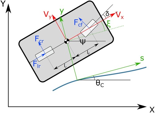
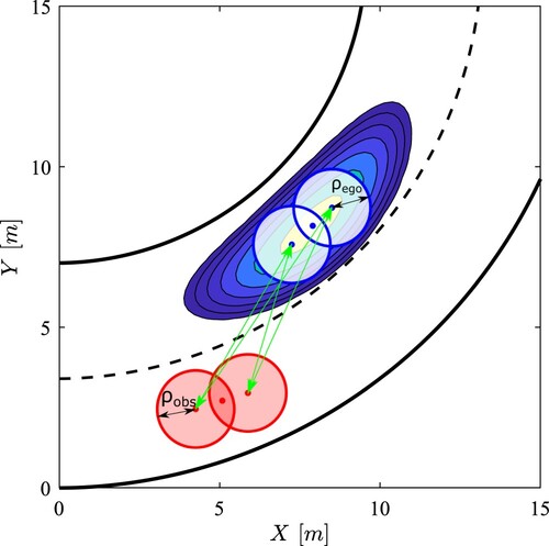
A reliable local road map is fundamental for the navigation of AVs and for the prediction of their position with respect to obstacles and to road boundaries along the optimisation horizon. Therefore, a local road map based has been developed in the local reference framework s-y (curvilinear abscissa and lateral displacement) as depicted in Figure 1). This framework is particularly convenient when describing road boundaries and obstacles' motion along the prediction horizon. Starting from a road map defined in the Cartesian global reference system X-Y, the local road map is generated by fitting third-order polynomials that locally approximate the road centreline angle ${\theta }_c$ as a function of the curvilinear abscissa s. This allows for a simple and effective, description of the road, while also ensuring continuity and derivability of road boundaries and static or moving obstacles in the optimisation problem.

Figure 1. Representation of the vehicle model framework. X-Y represents the global reference system, while s-y denotes the curvilinear abscissa reference system. $V_x$-$V_y$ are oriented according to the chassis' reference system.

Throughout this work, the complete knowledge of the road map is assumed. Thus, all the polynomial coefficients are available to the trajectory planner as a function of the vehicle's current position along the map. As stated in [35], considering the availability of a detailed road map is a reasonable assumption when dealing with the control of autonomous vehicles. This information can, for example, be obtained by combining off-line data and on-line information coming from a real-time environment mapping process based on vehicle mounted sensors such as cameras, lidars and radars [36,37].

2.2. Vehicle model

The vehicle model adopted in this work is a single-track dynamic model in which the lateral tyres forces are calculated through a simplified Pacejika's model based on a modified slip calculation procedure. This vehicle model represents a trade-off between the high complexity of 14 (or more) dofs models [38,39] and single-track kinematic models [27,40], allowing to reduce the number of state variables, while capturing the relevant nonlinearities associated with lateral tyre dynamics.

The model considers two translational dofs in the X-Y plane and one rotational dof around the Z axis as shown in Figure 1. The translation along the Z direction and the roll and pitch rotations are neglected. The system's equations of motion in state-space form $\dot{\mathit{x}}(t)=f(\mathit{x}(t),\mathit{u}(t))$, expressed in the local reference system s-y (see [41,42]) are reported in (1(1) $\begin{array}{rl}\dot{s}& ={\displaystyle \frac{V_x\cos (\xi )-V_y\sin (\xi )}{1-{\theta }_{cs}^{\mathrm{\prime }}y}}\\ \dot{y}& =V_x\sin (\xi )+V_y\cos (\xi )\\ \dot{\xi }& =\omega -{\theta }_{cs}^{\mathrm{\prime }}\dot{s}\\ \dot{V_x}& =\omega V_y+{\displaystyle \frac{F_{rl}}{M}}-{\displaystyle \frac{F_{fc}\sin (\delta )}{M}}-{\displaystyle \frac{F_{\mathrm{aero}}}{M}}\\ \dot{V_y}& =-\omega V_x+{\displaystyle \frac{F_{rc}}{M}}+{\displaystyle \frac{F_{fc}\cos (\delta )}{M}}\\ \dot{\omega }& ={\displaystyle \frac{1}{J_z}}(-F_{rc}{l}_r+F_{fc}{l}_f\cos (\delta ))\\ \dot{\delta }& =u_1\\ \dot{T_r}& =u_2\end{array}$(1) ), where $\mathit{x}(t)\in {\mathbb{R}}^8$ is the state vector and $\mathit{u}(t)\in {\mathbb{R}}^2$ is the input vector. (1) $\begin{array}{rl}\dot{s}& ={\displaystyle \frac{V_x\cos (\xi )-V_y\sin (\xi )}{1-{\theta }_{cs}^{\mathrm{\prime }}y}}\\ \dot{y}& =V_x\sin (\xi )+V_y\cos (\xi )\\ \dot{\xi }& =\omega -{\theta }_{cs}^{\mathrm{\prime }}\dot{s}\\ \dot{V_x}& =\omega V_y+{\displaystyle \frac{F_{rl}}{M}}-{\displaystyle \frac{F_{fc}\sin (\delta )}{M}}-{\displaystyle \frac{F_{\mathrm{aero}}}{M}}\\ \dot{V_y}& =-\omega V_x+{\displaystyle \frac{F_{rc}}{M}}+{\displaystyle \frac{F_{fc}\cos (\delta )}{M}}\\ \dot{\omega }& ={\displaystyle \frac{1}{J_z}}(-F_{rc}{l}_r+F_{fc}{l}_f\cos (\delta ))\\ \dot{\delta }& =u_1\\ \dot{T_r}& =u_2\end{array}$(1) with s is the curvilinear abscissa, y is the distance between the vehicle's centre of mass (C.o.M.) and the centreline, ξ is the error between the heading angle of the vehicle and the angle of the tangent to the road centreline in the global reference system ($\xi =\psi -{\theta }_c$), $V_x$, $V_y$ and ω are the vehicle's velocity components in the local reference system centred in the C.o.M., δ and $T_r$ are the steering angle at the front wheels and the torque applied to the rear axle and are obtained by integrating the inputs $u_1$ and $u_2$.

$T_r$ represents the total braking and accelerating torques applied to both front and rear axles. By neglecting the longitudinal slip, this allows to recover the total longitudinal braking and accelerating force $F_{rl}$ as $F_{rl}=T_r/R_r$, with $R_r$ the nominal wheels radius. This simplifying assumptions are acceptable in (relatively) low speed urban scenarios and avoid introducing additional dofs to describe the wheels' rotation.

The lateral forces $F_{fc}$ and $F_{rc}$ at the front and rear tyres are calculated using the well-known Pacejka's semi-empirical tyre model [31], also known as ‘Magic Formula’, considering steady-state pure lateral slip conditions: (2) $\begin{array}{r}{F}_{\ast c}=-2D\sin (C\mathrm{atan}(B{\alpha }_{\ast }+E(\mathrm{atan}(B{\alpha }_{\ast })-B{\alpha }_{\ast })))\end{array}$(2) where the pre-multiplication by 2 is used to take into account that there are two tyres for each axle, B, C, D, E are the Pacejka's coefficients and ${\alpha }_{\ast }$ is the slip angle of the front or rear tyres that are calculated as: (3) $\begin{array}{r}\begin{array}{rl}{\alpha }_f& =\mathrm{atan}\left(\frac{(V_y+\omega l_f)\cos (\delta )-V_x\sin (\delta )}{V_x\cos (\delta )+(V_y+\omega l_f)\sin (\delta )}\right)\\ {\alpha }_r& =\mathrm{atan}\left(\frac{V_y-\omega l_r}{V_x}\right)\end{array}\end{array}$(3) It is important to point out that equations (3(3) $\begin{array}{r}\begin{array}{rl}{\alpha }_f& =\mathrm{atan}\left(\frac{(V_y+\omega l_f)\cos (\delta )-V_x\sin (\delta )}{V_x\cos (\delta )+(V_y+\omega l_f)\sin (\delta )}\right)\\ {\alpha }_r& =\mathrm{atan}\left(\frac{V_y-\omega l_r}{V_x}\right)\end{array}\end{array}$(3) ) can be difficult to handle when $V_x\to 0m/s$. In fact, as $V_x$ approaches zero, the slips tend to infinity for non-vanishing $V_y$ or ω. This causes model instability even for small numerical or estimation errors.

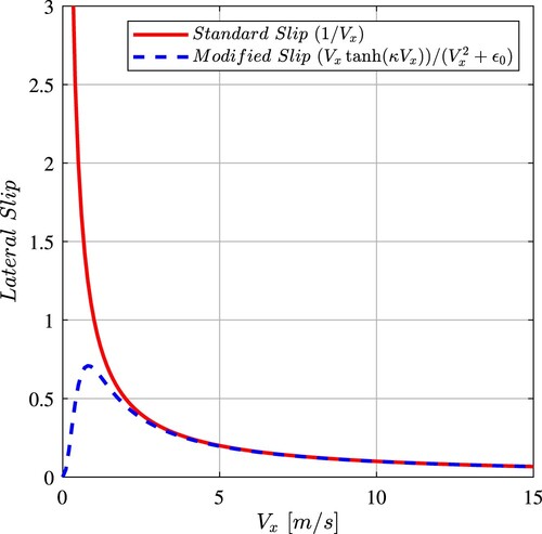
Since the intent is to develop a trajectory planner for urban environment, it is necessary to have a model that is robust and stable also at low or zero velocities. A velocity-dependent switch to a kinematic vehicle model would introduce additional computational costs and should therefore be avoided. Thus, the slip angle calculation has been modified as (4) $\begin{array}{rl}{\alpha }_f& =\mathrm{atan}\left(\frac{[(V_y+\omega l_f)\cos (\delta )-V_x\sin (\delta )]V_x\tanh (\kappa V_x)}{[V_x\cos (\delta )+(V_y+\omega l_f)\sin (\delta )]V_x+{ϵ}_0}\right)\\ {\alpha }_r& =\mathrm{atan}\left(\frac{[V_y-\omega l_r]V_x\tanh (\kappa V_x)}{V_x^2+{ϵ}_0}\right)\end{array}$(4) where κ and ${ϵ}_0$ allow to shape the transition toward a kinematic-like behaviour at low velocities while preserving the Pacejka's model slip calculation at medium–high speeds as shown in Figure 2.

Figure 2. Comparison between the standard and the modified slip curves with $\kappa =2$ and ${ϵ}_0=0.4$.

A table containing the main parameters considered is reported in Table 1.

Table 1. Values of the main model parameters.

M	860  kg	B	9.35
$J_z$	890  $kg{m}^2$	C	2.1
$l_f$	1.04  m	D	$2.06\exp (3)$
$l_r$	1.3  m	E	0.334
$R_r$	0.28  m	κ	2
		${ϵ}_0$	0.4

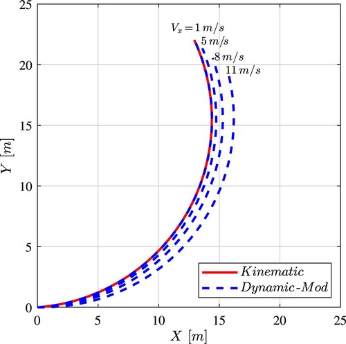
To assess the effectiveness of the modified slip calculation at low velocities, the dynamic vehicle model behaviour at different velocities is compared to the single-track kinematic vehicle model [27,40]. In Figure 3 are shown the vehicle C.o.M. trajectories obtained imposing a fixed reference steering input $\delta =0.15rad$ at the front wheels and constant longitudinal velocities $V_x=\{1,5,8,11\}m/s$. The effect of the lateral slip is clearly visible as the longitudinal velocity increases, while at (very) low velocities the dynamic model behaves like the kinematic one.

Figure 3. Comparison between the dynamic and the kinematic vehicle models C.o.M. trajectories obtained imposing a fixed reference steering input $\delta =0.15rad$ at the front wheels and constant longitudinal velocities $V_x=\{1,5,8,11\}m/s$.

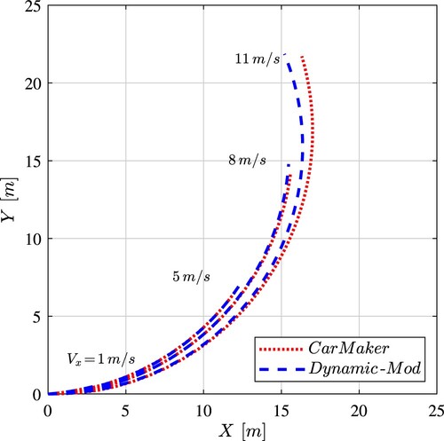
The single-track vehicle model with modified slip angle calculation has been also compared with an 18 dofs multibody vehicle model implemented in CarMaker environment. The results of the simulations are shown in Figure 4 where both models are subjected to a constant steering input $\delta =0.15rad$ at the front wheels and constant longitudinal velocities $V_x=\{1,5,8,11\}m/s$ for $3s$. At low velocities, the simplified 3 dofs model moves on trajectories that are very close to the ones of the more complex CarMaker model. As velocity increases, the single-track vehicle model predicts tighter curvature radii. This is due to the fact that the 3 dofs model does not account for the load transfers that cause a reduction of the tyre cornering stiffness [43]. The single-track vehicle trajectory at $11m/s$ has a curvature radius of $16.4m$, while a radius of $17.0m$ is obtained using the CarMaker model. It should be noted that this represents a pretty tough manoeuvre, that exploits approximately $73\mathrm{\%}$ of the tyre friction limit.

Figure 4. Comparison between CarMaker 18 dofs model and the dynamic single-track model with modified slip calculation C.o.M. trajectories for a fixed reference steering input $\delta =0.15rad$ at the front wheels and constant longitudinal velocities $V_x=\{1,5,8,11\}m/s$.

Since the trajectory planner has been designed for low to medium velocities in urban driving scenarios, the single-track vehicle model (1(1) $\begin{array}{rl}\dot{s}& ={\displaystyle \frac{V_x\cos (\xi )-V_y\sin (\xi )}{1-{\theta }_{cs}^{\mathrm{\prime }}y}}\\ \dot{y}& =V_x\sin (\xi )+V_y\cos (\xi )\\ \dot{\xi }& =\omega -{\theta }_{cs}^{\mathrm{\prime }}\dot{s}\\ \dot{V_x}& =\omega V_y+{\displaystyle \frac{F_{rl}}{M}}-{\displaystyle \frac{F_{fc}\sin (\delta )}{M}}-{\displaystyle \frac{F_{\mathrm{aero}}}{M}}\\ \dot{V_y}& =-\omega V_x+{\displaystyle \frac{F_{rc}}{M}}+{\displaystyle \frac{F_{fc}\cos (\delta )}{M}}\\ \dot{\omega }& ={\displaystyle \frac{1}{J_z}}(-F_{rc}{l}_r+F_{fc}{l}_f\cos (\delta ))\\ \dot{\delta }& =u_1\\ \dot{T_r}& =u_2\end{array}$(1) ) with the modified slip calculation (4(4) $\begin{array}{rl}{\alpha }_f& =\mathrm{atan}\left(\frac{[(V_y+\omega l_f)\cos (\delta )-V_x\sin (\delta )]V_x\tanh (\kappa V_x)}{[V_x\cos (\delta )+(V_y+\omega l_f)\sin (\delta )]V_x+{ϵ}_0}\right)\\ {\alpha }_r& =\mathrm{atan}\left(\frac{[V_y-\omega l_r]V_x\tanh (\kappa V_x)}{V_x^2+{ϵ}_0}\right)\end{array}$(4) ) represents a good approximation of the complex CarMaker model. Furthermore, differences between the estimated and the actual vehicle trajectories can be addressed by the feedback provided by the NMPC logic that, at each step, re-plans the optimal trajectory, compensating for small modelling errors and external disturbances.

2.3. Constraints

The OCP is subjected to both hard and soft constraints. In fact, soft constraints allow to obtain a smoother driving behaviour while improving the convergence of the solver and reducing the risk of hard constraints violations in the presence of modelling errors, external disturbances and uncertainties (eventually coming from sensors) related to obstacles' current and future estimated positions.

2.3.1. Box constraints on state and input variables

This set of constraints includes the physical limits of the vehicle model: (5) $\begin{array}{r}\{\begin{array}{lr}{\delta }_{min}\le \delta \le {\delta }_{max}& \text{(steering angle [rad])},\\ {T_r}_{min}\le T_r\le {T_r}_{max}& \text{(torque [Nm])},\\ {\dot{\delta }}_{min}\le \dot{\delta }\le {\dot{\delta }}_{max}& \text{(steering angular velocity [rad/s])},\\ {\dot{T_r}}_{min}\le \dot{T_r}\le {\dot{T_r}}_{max}& \text{(torque derivative [Nm/s])}.\end{array}\end{array}$(5)

Physical limits have been derived from the experimental vehicle presented in  [44,45] and they have been applied to both the simulated and the CarMaker multibody vehicle models as constraints. In this way, simulation results are already fitted on the real vehicle that, in a next phase of this work, will become the prototype on which this planner will be implemented.

The steering angle δ is limited by the geometry of the steering system while torque $T_r$ is bounded by the friction limit and the maximum torque that can be generated by the powertrain. The steering angular velocity $\dot{\delta }$ and the torque derivative $\dot{T_r}$ are limited according to the saturation limits of the actuators installed on the prototype vehicle. These constraints are handled by the active-set routine of the QP solver qpOASES [33].

2.3.2. Tyre force constraint

The coupling of the lateral and longitudinal tyre–road contact forces is indirectly accounted for by considering the coupling of the lateral and longitudinal accelerations through the equivalent friction ellipse constraint [46]: (6) $\begin{array}{r}\begin{array}{rl}{T}_r& \le R_{r}M[a_1\sqrt{1-\frac{{\dot{V}}_y^2}{b_1^2}}-[\omega V_y-\frac{F_{fc}\sin (\delta )}{M}-\frac{F_{\mathrm{aero}}}{M}]]\\ T_r& \ge R_{r}M[-a_2\sqrt{1-\frac{{\dot{V}}_y^2}{b_2^2}}-[\omega V_y-\frac{F_{fc}\sin (\delta )}{M}-\frac{F_{\mathrm{aero}}}{M}]]\end{array}\end{array}$(6) where coefficients $a_{\ast }$ and $b_{\ast }$ are fitted to approximate the ellipse-shaped envelope as a function of the estimated friction coefficient and road surface conditions. Note that the coefficients in the acceleration and braking phase can be different to account for the partitioning of the accelerating and braking torques between the two axles. Through (6(6) $\begin{array}{r}\begin{array}{rl}{T}_r& \le R_{r}M[a_1\sqrt{1-\frac{{\dot{V}}_y^2}{b_1^2}}-[\omega V_y-\frac{F_{fc}\sin (\delta )}{M}-\frac{F_{\mathrm{aero}}}{M}]]\\ T_r& \ge R_{r}M[-a_2\sqrt{1-\frac{{\dot{V}}_y^2}{b_2^2}}-[\omega V_y-\frac{F_{fc}\sin (\delta )}{M}-\frac{F_{\mathrm{aero}}}{M}]]\end{array}\end{array}$(6) ), the maximum total torque is constrained as a function of the lateral acceleration of the vehicle's C.o.M. This approach is acceptable in urban driving conditions (not in limit handling conditions) which in fact is the target for the proposed trajectory planner. This formulation can also be useful to enforce safety and improve robustness with respect to uncertain road conditions: as proposed in [47], the friction ellipse approximation could be artificially reduced with respect to the actual tyre-road friction limit to always maintain a safety margin. In the remainder of this work, only the nominal tyre-road friction parameters will be considered.

2.3.3. Presence of obstacles

Both static or moving obstacles (such as cars, trucks and motorcycles driving along the road as well as pedestrians crossing the road, vehicles parked on the road side, etc.) are taken into account. In the case of moving obstacles, it is fundamental to estimate not only the obstacle's current position, but also its future trajectory. The future obstacle's positions $s^{\mathrm{obs}}$ and $y^{\mathrm{obs}}$ in the local reference frame s-y are approximately obtained assuming constant obstacle's velocities $V_s^{\mathrm{obs}}$ and $V_y^{\mathrm{obs}}$ in the s and y-directions (simplest possible assumption) as in (7(7) $\begin{array}{r}\{\begin{array}{rl}{s}^{\mathrm{obs}}& =s_0^{\mathrm{obs}}+V_s^{\mathrm{obs}}t\\ y^{\mathrm{obs}}& =y_0^{\mathrm{obs}}+V_y^{\mathrm{obs}}t\end{array}\end{array}$(7) ). The adoption of the local s-y reference frame greatly simplifies the description of the obstacles' motion with respect to a more standard Cartesian reference system: two parameters are sufficient to reasonably approximate obstacles' motion even along twisty roads. (7) $\begin{array}{r}\{\begin{array}{rl}{s}^{\mathrm{obs}}& =s_0^{\mathrm{obs}}+V_s^{\mathrm{obs}}t\\ y^{\mathrm{obs}}& =y_0^{\mathrm{obs}}+V_y^{\mathrm{obs}}t\end{array}\end{array}$(7) Since Equations (7(7) $\begin{array}{r}\{\begin{array}{rl}{s}^{\mathrm{obs}}& =s_0^{\mathrm{obs}}+V_s^{\mathrm{obs}}t\\ y^{\mathrm{obs}}& =y_0^{\mathrm{obs}}+V_y^{\mathrm{obs}}t\end{array}\end{array}$(7) ) are time dependent, the equation $\dot{t}=1$ has been added to (1(1) $\begin{array}{rl}\dot{s}& ={\displaystyle \frac{V_x\cos (\xi )-V_y\sin (\xi )}{1-{\theta }_{cs}^{\mathrm{\prime }}y}}\\ \dot{y}& =V_x\sin (\xi )+V_y\cos (\xi )\\ \dot{\xi }& =\omega -{\theta }_{cs}^{\mathrm{\prime }}\dot{s}\\ \dot{V_x}& =\omega V_y+{\displaystyle \frac{F_{rl}}{M}}-{\displaystyle \frac{F_{fc}\sin (\delta )}{M}}-{\displaystyle \frac{F_{\mathrm{aero}}}{M}}\\ \dot{V_y}& =-\omega V_x+{\displaystyle \frac{F_{rc}}{M}}+{\displaystyle \frac{F_{fc}\cos (\delta )}{M}}\\ \dot{\omega }& ={\displaystyle \frac{1}{J_z}}(-F_{rc}{l}_r+F_{fc}{l}_f\cos (\delta ))\\ \dot{\delta }& =u_1\\ \dot{T_r}& =u_2\end{array}$(1) ) to integrate time along the prediction horizon. Note that the trajectory planner requires the knowledge of the obstacles' positions and velocities at each time sample. This information could be obtained from sensors installed on the vehicle (such as cameras, lidars and radars) [36,37].

One of the simplest yet effective ways to model the ego-vehicle and the obstacles is by means of multiple circles [26]. This method is highly flexible, as it allows to describe short vehicle (e.g. small city cars) and long vehicles (e.g. trams and trucks) by varying the number of circle used. If the ego-vehicle and the obstacle are both modelled with two circles, as shown in Figure 5, four circle-to-circle distance constraints are required for the collision constraint formulation. Most importantly, these can be easily reformulated as constraints on the distance between the centres of the circles, which can be practically approximated by the Euclidean distance in the s-y space. This is a fundamental advantage with respect to the description of the ego-vehicle and the obstacles by means of ellipses: while this method would only require one ellipse-to-ellipse distance constraint, it is not possible to obtain a closed-form analytic expression of such distance for arbitrary ego-vehicle and obstacle's orientations, preventing an efficient constraint implementation, thus ultimately affecting the solver usability.

Figure 5. Schematic representation of ego-vehicle and obstacle by means of multiple circles.

Each constraint is implemented both as a hard (8(8) $\begin{array}{rl}& (s_{c,\star }^{\mathrm{ego}}-s_{c,\star }^{\mathrm{obs}}{)}^2+(y_{c,\star }^{\mathrm{ego}}-y_{c,\star }^{\mathrm{obs}}{)}^2\ge ({\rho }^{\mathrm{ego}}+{\rho }^{\mathrm{obs}}{)}^2\end{array}$(8) ) and as a soft (9(9) $\begin{array}{rl}& C_{\mathrm{obs}}=e^{{\kappa }_{\mathrm{obs}}[({\rho }^{\mathrm{ego}}+{\rho }^{\mathrm{obs}}{)}^2-(s_{c,\star }^{\mathrm{ego}}-s_{c,\star }^{\mathrm{obs}}{)}^2-(y_{c,\star }^{\mathrm{ego}}-y_{c,\star }^{\mathrm{obs}}{)}^2]}\end{array}$(9) ) constraint: (8) $\begin{array}{rl}& (s_{c,\star }^{\mathrm{ego}}-s_{c,\star }^{\mathrm{obs}}{)}^2+(y_{c,\star }^{\mathrm{ego}}-y_{c,\star }^{\mathrm{obs}}{)}^2\ge ({\rho }^{\mathrm{ego}}+{\rho }^{\mathrm{obs}}{)}^2\end{array}$(8) (9) $\begin{array}{rl}& C_{\mathrm{obs}}=e^{{\kappa }_{\mathrm{obs}}[({\rho }^{\mathrm{ego}}+{\rho }^{\mathrm{obs}}{)}^2-(s_{c,\star }^{\mathrm{ego}}-s_{c,\star }^{\mathrm{obs}}{)}^2-(y_{c,\star }^{\mathrm{ego}}-y_{c,\star }^{\mathrm{obs}}{)}^2]}\end{array}$(9) where $s_{c,\star }$ and $y_{c,\star }$ (with $(\star )\in \{1,2\}$ indicating the two circles describing each car) represent the position of the centre of the circles of radii ${\rho }^{\mathrm{ego}}$ and ${\rho }^{\mathrm{obs}}$ . The position of the centres $s_{c,\star }$ and $y_{c,\star }$ is computed from the ego-vehicle and obstacle positions considering the ego-vehicle heading ψ and the approximated obstacle constant heading ${\psi }^{\mathrm{obs}}=\mathrm{atan}(V_y^{\mathrm{obs}}/V_s^{\mathrm{obs}})$, respectively. The soft constraint (9(9) $\begin{array}{rl}& C_{\mathrm{obs}}=e^{{\kappa }_{\mathrm{obs}}[({\rho }^{\mathrm{ego}}+{\rho }^{\mathrm{obs}}{)}^2-(s_{c,\star }^{\mathrm{ego}}-s_{c,\star }^{\mathrm{obs}}{)}^2-(y_{c,\star }^{\mathrm{ego}}-y_{c,\star }^{\mathrm{obs}}{)}^2]}\end{array}$(9) ) is implemented to improve the convergence speed of the solver, while the hard constraint is guarantees constraints satisfaction. The soft constraint is enforced by weighting $C_{\mathrm{obs}}$ in the cost function and it is designed to achieve a value of 1 when the hard constraint (8(8) $\begin{array}{rl}& (s_{c,\star }^{\mathrm{ego}}-s_{c,\star }^{\mathrm{obs}}{)}^2+(y_{c,\star }^{\mathrm{ego}}-y_{c,\star }^{\mathrm{obs}}{)}^2\ge ({\rho }^{\mathrm{ego}}+{\rho }^{\mathrm{obs}}{)}^2\end{array}$(8) ) is activated. The penalty term can be tuned by changing the value of the parameter ${\kappa }_{\mathrm{obs}}$ and by adjusting the weight in the cost function.

An extra soft constraint can be added as penalty in the cost function to enforce the minimum safety distance: (10) $\begin{array}{r}{C}_{\mathrm{safety}}=e^{{\kappa }_{\mathrm{safety}}[-d_s(s^{\mathrm{ego}}-s^{\mathrm{obs}}{)}^2-d_y(y^{\mathrm{ego}}-y^{\mathrm{obs}}{)}^2]}\end{array}$(10) This constraint is shaped as an ellipse in the s-y reference frame to guarantee to enforce the safety distance with respect to other vehicles also in tight curves as shown in Figure 5. The penalty term depends on the distance between the ego-vehicle position $s^{\mathrm{ego}}$–$y^{\mathrm{ego}}$ and the obstacle position $s^{\mathrm{obs}}$–$y^{\mathrm{obs}}$. Differently from the constraints (8(8) $\begin{array}{rl}& (s_{c,\star }^{\mathrm{ego}}-s_{c,\star }^{\mathrm{obs}}{)}^2+(y_{c,\star }^{\mathrm{ego}}-y_{c,\star }^{\mathrm{obs}}{)}^2\ge ({\rho }^{\mathrm{ego}}+{\rho }^{\mathrm{obs}}{)}^2\end{array}$(8) ) and (9(9) $\begin{array}{rl}& C_{\mathrm{obs}}=e^{{\kappa }_{\mathrm{obs}}[({\rho }^{\mathrm{ego}}+{\rho }^{\mathrm{obs}}{)}^2-(s_{c,\star }^{\mathrm{ego}}-s_{c,\star }^{\mathrm{obs}}{)}^2-(y_{c,\star }^{\mathrm{ego}}-y_{c,\star }^{\mathrm{obs}}{)}^2]}\end{array}$(9) ), the constraint  (10(10) $\begin{array}{r}{C}_{\mathrm{safety}}=e^{{\kappa }_{\mathrm{safety}}[-d_s(s^{\mathrm{ego}}-s^{\mathrm{obs}}{)}^2-d_y(y^{\mathrm{ego}}-y^{\mathrm{obs}}{)}^2]}\end{array}$(10) ) is meant to be used to actively promote a cautious and safer vehicle behaviour. This is done by the higher level behavioural layer that can adjust the ellipse parameters $d_s$, $d_y$, ${\kappa }_{\mathrm{safety}}$ and the penalty weight in the cost as a function of the ego-vehicle velocity, traffic conditions, visibility and maximum braking capability that usually depends on weather and road surface conditions. As an example, constraint (10(10) $\begin{array}{r}{C}_{\mathrm{safety}}=e^{{\kappa }_{\mathrm{safety}}[-d_s(s^{\mathrm{ego}}-s^{\mathrm{obs}}{)}^2-d_y(y^{\mathrm{ego}}-y^{\mathrm{obs}}{)}^2]}\end{array}$(10) ) can account for the uncertainty related to the obstacles' predicted velocities and future trajectories. In fact, while the obstacles' actual initial position estimation can be considered as being highly accurate (depending on the reliability of the sensors and of the estimation algorithms), the reliability of the prediction of future obstacles' positions relies on the assumption of constant velocities $V_s^{\mathrm{obs}}$ and $V_y^{\mathrm{obs}}$ . This uncertainty can be dealt with by reducing the weights $d_s$ and $d_y$ in Equation (10(10) $\begin{array}{r}{C}_{\mathrm{safety}}=e^{{\kappa }_{\mathrm{safety}}[-d_s(s^{\mathrm{ego}}-s^{\mathrm{obs}}{)}^2-d_y(y^{\mathrm{ego}}-y^{\mathrm{obs}}{)}^2]}\end{array}$(10) ), thus increasing the ellipse dimensions (e.g. as a function of time). In the remainder of this work, the weights $d_s$ and $d_y$ will be considered fixed and constant in time.

2.3.4. Road boundaries

The distance y of the road boundaries from the centreline as a function of the curvilinear abscissa s is described through third-order polynomials that are considered to be known as explained in Section 2.1. Similarly to the previous paragraph, the vehicle can be approximated with two circles of radius ${\rho }^{\mathrm{ego}}$. Therefore, for each of the two circles, the constraints of the left and right road boundaries can be written as: (11) $\begin{array}{r}\begin{array}{rl}& y_{c,\star }^{\mathrm{ego}}+{\rho }^{\mathrm{ego}}\le (K_{L,1}{s}^3+K_{L,2}{s}^2+K_{L,3}s+K_{L,4})\\ & y_{c,\star }^{\mathrm{ego}}-{\rho }^{\mathrm{ego}}\ge (K_{R,1}{s}^3+K_{R,2}{s}^2+K_{R,3}s+K_{R,4})\end{array}\end{array}$(11) with $K_{L,k}$ and $K_{R,k}$, k = 1, 2, 3, 4 coefficients of the left and right polynomials, respectively. Soft constraints are also implemented using an exponential function: (12) $\begin{array}{r}\begin{array}{rl}& C_{left,\star }=e^{{\kappa }_{\mathrm{road}}[y_{c,\star }^{\mathrm{ego}}+{\rho }^{\mathrm{ego}}-(K_{L,1}{s}^3+K_{L,2}{s}^2+K_{L,3}s+K_{L,4})]}\\ & C_{right,\star }=e^{{\kappa }_{\mathrm{road}}[-y_{c,\star }^{\mathrm{ego}}+{\rho }^{\mathrm{ego}}+(K_{R,1}{s}^3+K_{R,2}{s}^2+K_{R,3}s+K_{R,4})]}\end{array}\end{array}$(12) The penalty terms can be tuned by changing the value of the parameter ${\kappa }_{\mathrm{road}}$ and by adjusting the weight in the cost function.

2.4. Cost function

The cost function to be minimised is in the form of Bolza problem. Thus, it includes a quadratic integral term and a quadratic terminal term: (13) $\begin{array}{r}J=\frac{1}{2}{\int }_{t_0}^{t_f}(||\mathit{h}(\tau )-{\mathit{h}}_{\mathbf{r}\mathbf{e}\mathbf{f}}(\tau )|{|}_Q^2+||\mathit{u}(\tau )|{|}_R^2)d\tau +\frac{1}{2}||\mathit{h}(t_f)-{\mathit{h}}_{\mathbf{r}\mathbf{e}\mathbf{f}}(t_f)|{|}_P^2\end{array}$(13) where $||\bullet |{|}_{Q,R,P}^2$ denotes the Euclidean norm weighted with diagonal matrices Q, R or P. The input vector $\mathit{u}(t)\in {\mathbb{R}}^2$ accounts for the control actions, while ${\mathit{h}}^{\mathbf{\top }}(t)=[{\mathit{x}}^{\mathbf{\top }}(t),{\mathit{C}}^{\mathbf{s}\mathbf{o}\mathbf{f}\mathbf{t}\mathbf{\top }}(t)]$ is a time-dependent vector that contains the states $\mathit{x}(t)\in {\mathbb{R}}^8$ and the cost penalties ${\mathit{C}}^{\mathbf{s}\mathbf{o}\mathbf{f}\mathbf{t}}(t)\in {\mathbb{R}}^{N_{\mathrm{soft}}}$, and ${\mathit{h}}_{\mathbf{r}\mathbf{e}\mathbf{f}}(t)$ is the corresponding reference vector.

The elements of matrix Q that refer to the states are used to normalise the state error with respect to the maximum desired deviation $\mathrm{\Delta }{x}_{i_{max}}=x_{i_{max}}-h_{\mathrm{ref},i}$: (14) $\begin{array}{r}{Q}_{i,i}=\frac{1}{\mathrm{\Delta }{x}_{i_{max}}^2}\mathrm{for}i=1,\dots ,N_x.\end{array}$(14) In this way, the cost variation associated to an error equal to $\mathrm{\Delta }{x}_{i_{max}}$ is the same for all state variables. The remaining $N_{\mathrm{soft}}$ elements of the weight matrix Q are related to soft constraints. Recalling the definitions of soft constraints (9(9) $\begin{array}{rl}& C_{\mathrm{obs}}=e^{{\kappa }_{\mathrm{obs}}[({\rho }^{\mathrm{ego}}+{\rho }^{\mathrm{obs}}{)}^2-(s_{c,\star }^{\mathrm{ego}}-s_{c,\star }^{\mathrm{obs}}{)}^2-(y_{c,\star }^{\mathrm{ego}}-y_{c,\star }^{\mathrm{obs}}{)}^2]}\end{array}$(9) ) and (12(12) $\begin{array}{r}\begin{array}{rl}& C_{left,\star }=e^{{\kappa }_{\mathrm{road}}[y_{c,\star }^{\mathrm{ego}}+{\rho }^{\mathrm{ego}}-(K_{L,1}{s}^3+K_{L,2}{s}^2+K_{L,3}s+K_{L,4})]}\\ & C_{right,\star }=e^{{\kappa }_{\mathrm{road}}[-y_{c,\star }^{\mathrm{ego}}+{\rho }^{\mathrm{ego}}+(K_{R,1}{s}^3+K_{R,2}{s}^2+K_{R,3}s+K_{R,4})]}\end{array}\end{array}$(12) ), the values of the weights $Q_{i,i}$ for $i=N_x+1,\dots ,N_{\mathrm{soft}}$ represent the cost penalty associated with soft constraints with exponents equal to zero, i.e. the cost penalty associated with the activation of the corresponding hard constraints (8(8) $\begin{array}{rl}& (s_{c,\star }^{\mathrm{ego}}-s_{c,\star }^{\mathrm{obs}}{)}^2+(y_{c,\star }^{\mathrm{ego}}-y_{c,\star }^{\mathrm{obs}}{)}^2\ge ({\rho }^{\mathrm{ego}}+{\rho }^{\mathrm{obs}}{)}^2\end{array}$(8) ) and (11(11) $\begin{array}{r}\begin{array}{rl}& y_{c,\star }^{\mathrm{ego}}+{\rho }^{\mathrm{ego}}\le (K_{L,1}{s}^3+K_{L,2}{s}^2+K_{L,3}s+K_{L,4})\\ & y_{c,\star }^{\mathrm{ego}}-{\rho }^{\mathrm{ego}}\ge (K_{R,1}{s}^3+K_{R,2}{s}^2+K_{R,3}s+K_{R,4})\end{array}\end{array}$(11) ). This holds also for soft constraints that are not coupled with a hard constraint such as (10(10) $\begin{array}{r}{C}_{\mathrm{safety}}=e^{{\kappa }_{\mathrm{safety}}[-d_s(s^{\mathrm{ego}}-s^{\mathrm{obs}}{)}^2-d_y(y^{\mathrm{ego}}-y^{\mathrm{obs}}{)}^2]}\end{array}$(10) ).

The reference vector ${\mathit{h}}_{\mathbf{r}\mathbf{e}\mathbf{f}}$ is, in general, time dependent. All reference values related to soft constraints are set to zero. The reference for ξ, $V_y$, ω, δ, $T_r$ and all reference values related to soft constraints are set to zero. Instead, the reference value of y can be different from zero in case of roads with multiple lanes. Similarly, the reference value of $V_x$ is set to be equal to a desired speed profile while the reference value of the curvilinear position s is set to be equal to the time integral of the velocity or to an arbitrary value if the associated weight in matrix Q is null.

The weight matrix R can be chosen in the same way as done for the matrix Q considering that the references for both control actions is zero.

Finally, matrix P can be, for example, obtained as the solution of Riccati equation for the infinite time LQR problem considering the system's equations linearised around the steady-state condition $\mathit{x}=\mathbf{0}$ and weight matrices Q and R.

3. Algorithm implementation

3.1. Perceived and simulated spatial horizons

While developing a trajectory planner for autonomous driving, it is important to consider the difference between the horizon perceived by the sensors and the one simulated within the NMPC. In particular, the former depends on the range of the sensors (such as cameras, lidars and radars) while the latter is defined by two parameters: the time span of the optimisation horizon, which is generally fixed a priori, and the vehicle velocity, which is not known beforehand being a consequence of the optimisation process itself. It is clear that, for safety reasons, the simulated spatial horizon should be shorter than the perceived one, thus allowing to plan trajectories only within the ‘known’ environment. Limiting the simulated spatial horizon length by imposing a constraint on the maximum travelled distance s at the final time $t_f$ can be problematic. The combination of warm starting the solver with the previous step optimal trajectory coupled with quick changes in the perceived spatial horizon length (e.g. due to the scene understanding and vision algorithms) can result in an infeasible optimisation problem or in solver timeouts.

This issue can be addressed by transforming the OCP into a spatial dependent one as in [23,25]. As already pointed out, this approach implies strong assumptions on the velocity profile of the vehicle and cannot be easily integrated in a controller for urban driving.

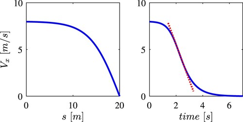
In order not to switch to a spatial OCP, the simulated spatial horizon is limited by imposing an extra inequality constraint on the velocity $V_x$ as a function of the curvilinear abscissa s as in (15(15) $\begin{array}{r}{V}_x\le V_{x_{max}}\tanh ({\kappa }_{\mathrm{vel}}(s-s_{max}))\end{array}$(15) ). The velocity profile constraint enforces a deceleration that achieves zero velocity at the desired abscissa $s_{max}$. (15) $\begin{array}{r}{V}_x\le V_{x_{max}}\tanh ({\kappa }_{\mathrm{vel}}(s-s_{max}))\end{array}$(15) The reference velocity $V_{x_{max}}$ is set by the behavioural layer as the maximum allowed speed considering road rules and estimated tyre-road friction coefficient. The parameter ${\kappa }_{vel}$ is used to limit the resulting maximum deceleration imposed by the velocity profile within comfort limits. In Figure 6 examples of spatial and temporal velocity profiles for $V_{x_{max}}=8m/s$ and $s_{max}=20m$ are shown. Differently from a constant deceleration, this profile provides a much smoother deceleration, especially toward the end of the braking phase, reducing harshness and improving passengers' comfort.

Figure 6. Spatial and temporal velocity profiles.

3.2. Driving modes

A driving mode is composed by a set of parameters comprising safety distance soft constraints coefficients such as ${\kappa }_{\mathrm{safety}}$, $d_s$, $d_y$, velocity constraints parameters $V_{x_{max}}$, $s_{max}$, ${\kappa }_{\mathrm{vel}}$, and weighting matrices matrices Q, R, P. The concept of driving mode has been developed to adapt the NMPC trajectory planner to a wide range of driving conditions. The driving mode is selected by the higher level behavioural layer considering road rules, traffic, visibility, weather and road surface conditions. The switching between modes is accomplished by gradually shifting from the parameters of one mode to ones of the other. In this way the continuity between subsequent solutions is maintained and sharp discontinuities are avoided, resulting in a more natural and comfortable driving behaviour.

Two driving modes will be considered in this work: the DRIVE and the OVERTAKE modes. The DRIVE mode is used to drive along the road, keeping the current lane and reducing the vehicle's velocity if a slower preceding vehicle is detected. The OVERTAKE mode, instead, is used to overtake slower preceding vehicles if possible. For the sake of exposition, the following numerical examples do not tackle the problem of mode selection and the selected mode is maintained throughout the whole manoeuvre.

3.3. Numerical solution

The resulting finite horizon OCP that has to be solved at each NMPC iteration is the following: (16a) $\begin{array}{rl}\underset{\mathit{u}(t)}{\mathrm{minimise}}& \frac{1}{2}{\int }_{t_0}^{t_f}(||\mathit{h}(\tau )-{\mathit{h}}_{\mathbf{r}\mathbf{e}\mathbf{f}}(\tau )|{|}_Q^2+||\mathit{u}(\tau )|{|}_R^2)d\tau \\ & +\frac{1}{2}||\mathit{h}(t_f)-{\mathit{h}}_{\mathbf{r}\mathbf{e}\mathbf{f}}(t_f)|{|}_P^2\end{array}$(16a) (16b) $\begin{array}{rl}\text{subject to:}& \dot{\mathit{x}}(t)=f(\mathit{x}(t),\mathit{u}(t))\end{array}$(16b) (16c) $\begin{array}{rl}& \mathit{x}(t_0)={\mathit{x}}_{\mathbf{0}}\end{array}$(16c) (16d) $\begin{array}{rl}& {\mathit{x}}_{\mathbf{min}}(t)\le \mathit{x}(t)\le {\mathit{x}}_{\mathbf{max}}(t)\end{array}$(16d) (16e) $\begin{array}{rl}& {\mathit{u}}_{\mathbf{min}}(t)\le \mathit{u}(t)\le {\mathit{u}}_{\mathbf{max}}(t)\end{array}$(16e) (16f) $\begin{array}{rl}& \mathit{g}(t)\le \mathbf{0}\end{array}$(16f)

The OCP is iteratively solved in an MPC framework using the open source ACADO toolkit software that implements Bock's multiple shooting method [48] coupled with Real-Time Iteration (RTI) scheme [49–51].

The RTI scheme is based on a sequential quadratic programming (SQP) method that performs only one iteration per sampling time, reinitialising the trajectory by shifting the old prediction. In particular, each RTI iteration is divided into a preparation and a feedback phase. The preparation phase is performed before the new sample is available and takes care of computationally expensive tasks, such as sensitivities generation and matrix condensation. The feedback phase is performed, as soon as the new sample is available, by solving the updated small-scale parametric QP problem. In this case, the small-scale QP problem has been solved with the QP solver qpOASES [33], an open source C++ implementation of an on-line active-set strategy based on a parametric quadratic programming approach [52].

The ACADO Code Generation tool produces a self-contained C-code. The computational speed is increased exploiting automatic differentiation and avoiding dynamic memory allocation by hard-coding all problem dimensions [32].

3.4. Improved robustness

Rapid changes in the constraints can easily make the previous time-step solution infeasible. Given that a shifted version of such solution is used as the warm-start initialisation for the next iteration, this might lead to a condition where the solver cannot recover an obstacle free path that satisfies the new constraints. This issue is related to the high nonlinearity of the problem and the extremely complex and non-convex feasible domain. A typical urban-driving scenario that can induce this type of infeasibility, causing a solver error, is the case of an obstacle that suddenly appears within the simulated spatial horizon, e.g. a pedestrian suddenly crossing the street or another vehicle performing a hazardous overtaking manoeuvre. For these reasons, it is necessary to set up a backup policy that allows, if possible, to find a feasible solution to the planning task, even in the presence of this edge-case scenarios.

A possibility could be to reinitialise, at each iteration, the solver warm-start trajectory with identical copies of the current estimated state along the whole prediction horizon. This method can be successfully applied for low-speed manoeuvres with short simulated spatial horizons in particularly crowded environments, such as a restart after a traffic stop light. Unfortunately, as the spatial horizon and the longitudinal velocity increase ($V_x⪆2m/s$), this method would require too many QP iterations to converge to a locally optimal solution.

An alternative approach is to have multiple identical sub-planners with different simulated spatial horizon lengths that work in parallel. This is achieved by enforcing to each sub-planner a different velocity constraint in the form (15(15) $\begin{array}{r}{V}_x\le V_{x_{max}}\tanh ({\kappa }_{\mathrm{vel}}(s-s_{max}))\end{array}$(15) ). Considering a configuration with three sub-planners, A, B and C, three velocity constraints are generated by imposing three different spatial horizon lengths $s_{max}^A>s_{max}^B>s_{max}^C$. For example $s_{max}^A$ could be set as the maximum available perceived spatial horizon length, while $s_{max}^C$ could correspond to the minimum stopping distance calculated considering the current vehicle's velocity and maximum admissible deceleration. The solution adopted is the one given by the sub-planner with the longest spatial horizon that obtained a feasible trajectory within a predefined computational time budget. The effectiveness of this approach will be further analyzed with a simulation example in the next section.

4. Simulation results

The NMPC described in previous sections is implemented considering a time horizon length of $3s$ discretised in N = 60 steps (thus $\mathrm{\Delta }t=0.05s$). The temporal horizon length is a design parameter that should be chosen considering the range of the sensors and the stopping distance of the vehicle (a function of tyre-road friction coefficient and velocity). The forward integration of the system's dynamics is accomplished by second order implicit Runge–Kutta method and two full sequential quadratic programming (SQP) iterations are performed per NMPC step. Thus, the vehicle's inputs are updated at a frequency of $20Hz$, applying the first of the 60 calculated optimal control actions.

All closed-loop simulations are performed considering a detailed 18 dofs CarMaker model. Ego-vehicle state and obstacles positions and velocities are directly computed by the simulator and assumed as known. In [53] a real implementation of and estimator for these quantities based on a Kalman filter algorithm that combines lidars and radars data is presented. Simulations are performed on a laptop featuring an Intel i7-3610QM CPU and 8 GB of RAM.

In the following, two relevant driving scenarios are considered.

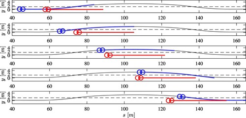
4.1. Overtaking of a single moving obstacle

In this first scenario, the ego-vehicle is required to overtake a moving obstacle positioned at a distance $\mathrm{\Delta }s=25m$, in the same lane as the ego-vehicle, with constant longitudinal velocity $V_{s_{\mathrm{obs}}}=10m/s$ and zero lateral velocity. The reference longitudinal velocity of ego-vehicle is set to $V_{x_{\mathrm{ref}}}=13m/s$ and a straight road is considered for the sake of representation clarity.

The weight matrix of the OVERTAKE mode and a sufficiently long perceived spatial horizon allow a safe overtaking manoeuvre, during which the safety distance from the obstacle is always maintained. The ego-vehicle and obstacle trajectories, together with the predictions along the optimisation horizon, are displayed in Figure 7.

Figure 7. Ego-vehicle and obstacle trajectories during the overtaking manoeuvre.

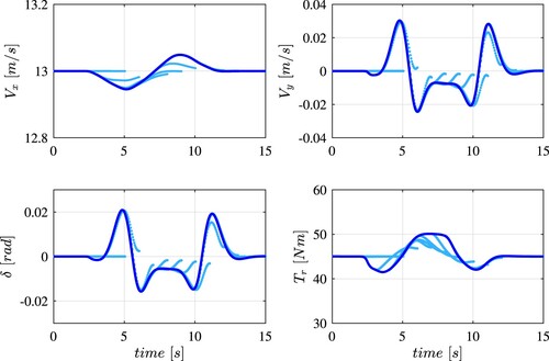
The velocities $V_x$ and $V_y$, the steering angle δ and the applied torque $T_r$ as functions of time are presented in Figure 8. The velocity of the ego-vehicle remains approximately constant and the lateral displacement is increased up to $y=3.4m$ to keep the appropriate safety distance from the obstacle during the overtaking manoeuvre.

Figure 8. Longitudinal velocity $V_x$, lateral velocity $V_y$, steering angle at the wheels δ and rear axle torque $T_r$ during the overtake manoeuvre. The closed-loop states trajectory is shown by the dark solid line, while the light dotted lines show the finite-length 60-steps optimal NMPC predictions. The controller runs at $20Hz$, but only one every 20 optimal predictions is shown to improve clarity.

The computational time required to solve each OCP is, on average, lower than $8ms$. Therefore, the real-time feasibility of the proposed trajectory planner can be stated.

4.2. Car suddenly exiting from a blind spot

The parallel sub-planners configuration proposed in Section 3.4 is now assessed considering three sub-planners, A, B and C with velocity constraints defined by a common $V_{x_{max}}=9m/s$ and spatial horizon lengths $s_{max}^A=30m$, $s_{max}^B=15m$ and $s_{max}^C=10m$, respectively. Aiming at reducing the computational burden of this configuration, only the sub-planner with the longest spatial horizon performs two full SQP iterations, while the other two implement only one SQP iteration. A maximum CPU-time of 10/ms is allowed for each sub-planner, if a sub-planner cannot provide a feasible solution within this time limit, a timeout occurs and the sub-planner is declared infeasible.

The simulation test is performed on a straight road along which the ego-vehicle is driving at the reference speed of $V_{x_{\mathrm{ref}}}=8m/s$. An obstacle suddenly appears from the right side of the road at a distance $\mathrm{\Delta }s=20m$. The obstacle travels at $3m/s$ and enters the ego-vehicle lane without observing the right of way prescribed by the yield sign as shown in Figure 9. Due to the presence of a building, the field of view of the ego-vehicle is obstructed and the other vehicle is detected only at $t=1.2s$. This causes an infeasibility in sub-planner A that cannot compute a feasible solution within the prescribed $10ms$ as shown in Figure 11. In these conditions, sub-planners B and C can still provide feasible solutions, thus, the planned optimal inputs of sub-planner B are adopted. For t>1.2s, sub-planned B becomes the leading planner and its spatial horizon is extended to $s_{max}^{B_{t>1.2}}=30m$ and will perform two SQP iterations, while sub-planner A is declassed to a spatial horizon equal to $s_{max}^{A_{t>1.2}}=15m$ and one SQP iteration.

Figure 9. Ego-vehicle and obstacle trajectories. The obstacle suddenly appears on the side of the ego-vehicle due to an obstruction of its field of view.

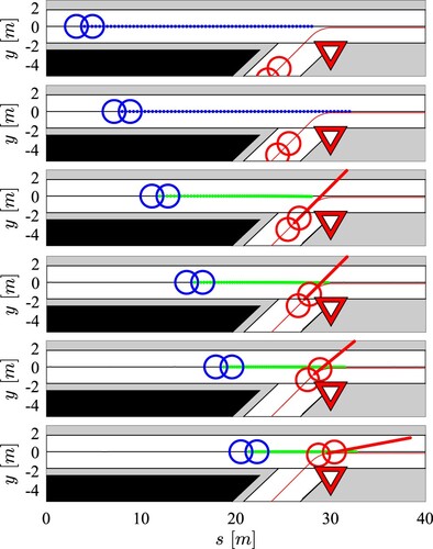
Figure 10. Longitudinal velocity $V_x$, lateral velocity $V_y$, steering angle at the wheels δ and rear axle torque $T_r$ during the emergency manoeuvre. At $t=1.2s$ sub-planner A cannot find a feasible solution. Thus, the solution provided by sub-planner B is used instead.

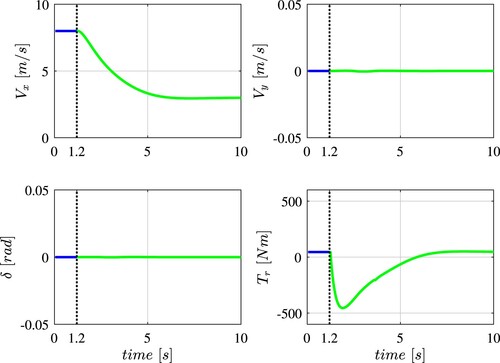
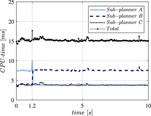
Figure 11. Sub-planner A, sub-planner B, sub-planner C and total trajectory planner CPU-time. After t = 1.2s sub-planner B becomes the leading planner with the longer spatial horizon and two SQP iterations per cycle.

The ego-vehicle and obstacle trajectories, together with their prediction along the optimisation horizon, are displayed in Figure 9. Note that, as explained in Section 2, the obstacle trajectory is approximated at each step with constant velocities in both longitudinal and lateral directions.

Figure 10, instead, shows the velocities $V_x$ and $V_y$, the steering angle δ and the applied torque $T_r$ during the braking manoeuvre. The longitudinal velocity is reduced to match the speed of the merging vehicle, generating a longitudinal deceleration of approximately $6.5m/s^2$, which is still within the adhesion limit of the tyres.

Figure 11 shows that, even without considering the possible sub-planner parallelisation, the total computational time, obtained by summing the three CPU-times as would be the case in a sequential implementation, is lower than $20ms$, thus well below the total iteration available time of $50ms$. Therefore, even this more complex configuration of the trajectory planner can be implemented within the real-time control framework of an autonomous vehicle.

5. Conclusions and future works

In this paper an NMPC trajectory planner for autonomous vehicles based on a direct approach has been presented. Thanks to the proposed modified slip calculation, the dynamic single-track vehicle model can be employed at both high and low velocities. This allows to have one single model that presents a kinematic-like behaviour at low velocities while keeping the standard dynamic single-track vehicle model behaviour at higher speeds. Obstacles' uncertainties have been taken into account through the implementation of coupled soft and hard constraints. The correlation between the simulated and perceived spatial horizon lengths has been enforced with a spatial-dependent velocity profile that has been imposed as an extra inequality constraint. The numerical solution is carried out using ACADO toolkit, coupled with the QP solver qpOASES. The trajectory planner performances have been checked in simulation, applying the controller to a nonlinear multibody model in CarMaker environment. The results coming from the simulations carried on two significant driving scenarios have been reported to highlight the effectiveness of the calculated trajectories. The particular formulation with continuous and differentiable analytic functions introduced for the dynamics, for the road geometry and boundaries and for the obstacles allowed to use automatic differentiation, and therefore efficiently exploit the high performance QP solver. The trajectory planner with three parallel sub-planners showed improved robustness, while the analysis of the computational times has confirmed that it can be feasibly implemented within the real-time control routine of an autonomous vehicle.

Ongoing and future works include an extensive experimental campaign to obtain an improved identification of the model parameters and further validation of the proposed algorithms on an experimental autonomous vehicle. Potential developments are the implementation of high-level logics based on finite state machines to deal with multiple urban-driving scenarios and the integration of state estimation and obstacles' behaviour uncertainties in the planning algorithm.

Acknowledgements

The Italian Ministry of Education, University and Research is acknowledged for the support provided through the Project ‘Department of Excellence LIS4.0 – Lightweight and Smart Structures for Industry 4.0’.

Disclosure statement

No potential conflict of interest was reported by the author(s).

References

- Harper CD, Hendrickson CT, Mangones S, et al. Estimating potential increases in travel with autonomous vehicles for the non-driving, elderly and people with travel-restrictive medical conditions. Transp Res C. 2016;72:1–9.
- Greenblatt JB, Shaheen S. Automated vehicles, on-demand mobility, and environmental impacts. Current Sustainable/renewable Energy Reports. 2015;2(3):74–81.
- Paden B, Čáp M, Yong SZ, et al. A survey of motion planning and control techniques for self-driving urban vehicles. IEEE Trans Intel Vehicles. 2016;1(1):33–55.
- Li X, Sun Z, Cao D, et al. Development of a new integrated local trajectory planning and tracking control framework for autonomous ground vehicles. Mech Syst Signal Process. 2017;87:118–137.
- Khatib O. Real-time obstacle avoidance for manipulators and mobile robots. Proceedings of the 1985 IEEE International Conference on Robotics and Automation. Vol. 2. IEEE; 1985. p. 500–505.
- Borenstein J, Koren Y. Real-time obstacle avoidance for fast mobile robots. IEEE Trans Syst Man Cybern. 1989;19(5):1179–1187.
- Borenstein J, Koren Y. The vector field histogram-fast obstacle avoidance for mobile robots. IEEE Trans Rob Autom. 1991;7(3):278–288.
- Koren Y, Borenstein J. Potential field methods and their inherent limitations for mobile robot navigation. Proceedings, 1991 IEEE International Conference on Robotics and Automation. IEEE; 1991, p. 1398–1404.
- Judd K, McLain T. Spline based path planning for unmanned air vehicles. AIAA Guidance, Navigation, and Control Conference and Exhibit; 2001. p. 4238.
- Fleury S, Soueres P, Laumond JP, et al. Primitives for smoothing mobile robot trajectories. IEEE Trans Rob Autom. 1995;11(3):441–448.
- LaValle SM. Rapidly-exploring random trees: a new tool for path planning. The Annual Research Report. 1998.
- Karaman S, Frazzoli E. Optimal kinodynamic motion planning using incremental sampling-based methods. 2010 49th IEEE Conference on Decision and Control (CDC). IEEE; 2010. p. 7681–7687.
- Berntorp K. Path planning and integrated collision avoidance for autonomous vehicles. 2017 American Control Conference (ACC). IEEE; 2017. p. 4023–4028.
- Pepy R, Lambert A, Mounier H. Path planning using a dynamic vehicle model. 2006 2nd International Conference on Information & Communication Technologies. Vol. 1. IEEE; 2006. p. 781–786.
- Nagy B, Kelly A. Trajectory generation for car-like robots using cubic curvature polynomials. Field and Service Robots. 2001;11:479–490.
- Chen C, He Y, Bu C, et al. Quartic bézier curve based trajectory generation for autonomous vehicles with curvature and velocity constraints. 2014 IEEE International Conference on Robotics and Automation (ICRA). IEEE; 2014. p. 6108–6113.
- Alia C, Gilles T, Reine T, et al. Local trajectory planning and tracking of autonomous vehicles, using clothoid tentacles method. 2015 IEEE Intelligent Vehicles Symposium (IV). IEEE; 2015. p. 674–679.
- De Doná J, Suryawan F, Seron M, et al. A flatness-based iterative method for reference trajectory generation in constrained NMPC. In: Nonlinear model predictive control. Springer; 2009. p. 325–333.
- Qian X, Navarro I, de La Fortelle A, et al. Motion planning for urban autonomous driving using bézier curves and MPC. 2016 IEEE 19th International Conference on Intelligent Transportation Systems (ITSC). IEEE; 2016. p. 826–833.
- Falcone P, Borrelli F, Asgari J, et al. Predictive active steering control for autonomous vehicle systems. IEEE Trans Control Syst Technol. 2007;15(3):566–580.
- Falcone P, Borrelli F, Asgari J, et al. Low complexity MPC schemes for integrated vehicle dynamics control problems. 9th International Symposium on Advanced Vehicle Control; 2008.
- Liniger A, Domahidi A, Morari M. Optimization-based autonomous racing of 1: 43 scale rc cars. Optim Control Appl Methods. 2015;36(5):628–647.
- Frasch JV, Gray A, Zanon M, et al. An auto-generated nonlinear MPC algorithm for real-time obstacle avoidance of ground vehicles. 2013 European Control Conference (ECC). IEEE; 2013. p. 4136–4141.
- Gray A, Gao Y, Lin T, et al. Predictive control for agile semi-autonomous ground vehicles using motion primitives. American Control Conference (ACC), 2012. IEEE; 2012. p. 4239–4244.
- Gao Y, Gray A, Frasch JV, et al. Spatial predictive control for agile semi-autonomous ground vehicles. Proceedings of the 11th International Symposium on Advanced Vehicle Control; 2012.
- Gutjahr B, Gröll L, Werling M. Lateral vehicle trajectory optimization using constrained linear time-varying MPC. IEEE Trans Intell Transp Syst. 2017;18(6):1586–1595.
- Kong J, Pfeiffer M, Schildbach G, et al. Kinematic and dynamic vehicle models for autonomous driving control design. Intelligent Vehicles Symposium; 2015. p. 1094–1099.
- Inghilterra G, Arrigoni S, Braghin F, et al. Firefly algorithm-based nonlinear MPC trajectory planner for autonomous driving. 2018 International Conference of Electrical and Electronic Technologies for Automotive; 2018. p. 1–6.
- Arrigoni S, Trabalzini E, Bersani M, et al. Non-linear MPC motion planner for autonomous vehicles based on accelerated particle swarm optimization algorithm. 2019 AEIT International Conference of Electrical and Electronic Technologies for Automotive (AEIT AUTOMOTIVE); 2019. p. 1–6.
- Arrigoni S, Braghin F, Cheli F. MPC trajectory planner for autonomous driving solved by genetic algorithm technique. Vehicle Syst Dyn [Internet]. 2021;1–26. Available from:https://doi.org/10.1080/00423114.2021.1999991.
- Pacejka HB, Bakker E. The magic formula tyre model. Vehicle Syst Dyn. 1992;21(S1):1–18.
- Houska B, Ferreau HJ, Diehl M. Acado toolkit–an open-source framework for automatic control and dynamic optimization. Optim Control Appl Methods. 2011;32(3):298–312.
- Ferreau HJ, Kirches C, Potschka A, et al. qpoases: a parametric active-set algorithm for quadratic programming. Math Program Comput. 2014;6(4):327–363.
- Carmaker 7.0.2. IPG Automotive GmbH. Karlsruhe, Germany. https://ipg-automotive.com/.
- Jo K, Lee M, Kim J, et al. Tracking and behavior reasoning of moving vehicles based on roadway geometry constraints. IEEE Trans Intell Transp Syst. 2017;18(2):460–476.
- Mentasti S, Matteucci M. Multi-layer occupancy grid mapping for autonomous vehicles navigation. 2019 International Conference of Electrical and Electronic Technologies for Automotive. IEEE; 2019.
- Kocić J, Jovičić N, Drndarević V. Sensors and sensor fusion in autonomous vehicles. 2018 26th Telecommunications Forum (TELFOR). IEEE; 2018. p. 420–425.
- Braghin F, Cheli F, Leo E, et al. Dinamica dell'autoveicolo. 2009.
- Shim T, Ghike C. Understanding the limitations of different vehicle models for roll dynamics studies. Vehicle Syst Dyn. 2007;45(3):191–216.
- Rajamani R. Vehicle dynamics and control. Springer Science & Business Media; 2011.
- Nilsson NJ. Shakey the robot. 1984. (Technical Report, no. 323). Available from https://ci.nii.ac.jp/naid/10004211424/en/.
- Micaelli A, Samson C. Trajectory tracking for unicycle-type and two-steering-wheels mobile robots [PhD dissertation]. INRIA; 1993.
- Ploechl M. Road and off-road vehicle system dynamics handbook (G. Mastinu, editor) (1st ed.). CRC Press; 2014. https://doi.org/10.1201/b15560.
- Arrigoni S, Mentasti S, Cheli F, et al. Design of a prototypical platform for autonomous and connected vehicles. 2021 AEIT International Conference on Electrical and Electronic Technologies for Automotive (AEIT AUTOMOTIVE); 2021. p. 1–6.
- Vignati M, Tarsitano D, Cheli F. On how to transform a commercial electric quadricycle into a full autonomously actuated vehicle. 14th International Symposium on Advanced Vehicle Control (AVEC'18); 2018. p. 1–7.
- Brach RM, Brach RM. Modeling combined braking and steering tire forces. SAE Technical Paper; 2000. (Tech. Rep.).
- Brach R, Brach M. The tire-force ellipse (friction ellipse) and tire characteristics. SAE Technical Paper; 2011. (Tech. Rep.).
- Bock HG, Plitt KJ. A multiple shooting algorithm for direct solution of optimal control problems. IFAC Proceedings Volumes. 1984;17(2):1603–1608.
- Diehl M, Bock HG, Schlöder JP, et al. Real-time optimization and nonlinear model predictive control of processes governed by differential-algebraic equations. J Process Control. 2002;12(4):577–585.
- Diehl M, Bock HG, Schlöder JP. A real-time iteration scheme for nonlinear optimization in optimal feedback control. SIAM J Control Optim. 2005;43(5):1714–1736.
- Diehl M, Findeisen R, Allgöwer F. A stabilizing real-time implementation of nonlinear model predictive control. In: Real-time PDE-constrained optimization. SIAM; 2007. p. 25–52.
- Best MJ. An algorithm for the solution of the parametric quadratic programming problem. In: Applied mathematics and parallel computing. Springer; 1996. p. 57–76.
- Bersani M, Mentasti S, Dahal P, et al. An integrated algorithm for ego-vehicle and obstacles state estimation for autonomous driving. Rob Auton Syst. 2021;139. Article Id 103662. Available from: https://www.sciencedirect.com/science/article/pii/S0921889020305029.