Replacement optimization of ageing infrastructure under differential inflation

Abstract

Ageing public infrastructure assets necessitate economic replacement analysis. A common replacement problem concerns an existing asset challenged by a replacement option. Classic techniques obtained from the domain of engineering economics are the mainstream approach to replacement optimization in practice. However, the validity of these classic techniques is built on the assumption that life cycle cash flows of a replacement option are repetitive. Differential inflation undermines this assumption and therefore more advanced replacement optimization techniques are required under these circumstances. These techniques are found in the domain of operations research and require linear or dynamic programming (LP/DP). Since LP/DP techniques are complex and time-consuming, the current study develops an alternative model for replacement optimizations under differential inflation. This approach builds on the classic capitalized equivalent replacement technique. The alternative model is validated by comparison with a DP model showing to be equally accurate for a case with characteristics that apply to many infrastructure assets.

Keywords:

• Replacement decisions
• public infrastructure assets
• differential inflation
• asset management
• optimization

Introduction

Public sector organizations confront ageing infrastructure assets. Infrastructure assets, once built, often need to be replaced at the end of their economic or functional life, whichever comes first. The economic life is determined by a life cycle cost calculation. An asset is at the end of its economic life when it becomes less expensive to replace it with an equivalent alternative (Park 2011, Hartman and Tan 2014). In contrast, functional life is reached when an asset is not able to fulfil its original function (Lemer 1996). In addition, the functional service life designates the time-period in which a certain function such as transportation, high water protection or water crossing should be provided. In this context, the functional service life is the life cycle of a users’ system which incorporates multiple successive infrastructure assets’ life cycles (Wasson 2016).

Replacement decisions are time-variant optimization challenges of such a system. The purpose of an economic replacement analysis is to assess whether postponing a replacement justifies the cost of lifetime extension, major overhauls and renovations and for how long. This type of replacement problem is commonly designated a defender-challenger replacement analysis. A defender is the existing asset that can remain in service for a limited number of years with a major overhaul or renovation; a challenger is the replacement option.

Replacement analyses are a special class of problems in the field of engineering economics, and the literature offers an array of fundamental and advanced calculation approaches that are applicable under specific circumstances. However, for cost engineers, economic replacement analysis is challenging for such reasons as selecting the correct calculation technique in relation to the specific circumstances and understanding of inflationary effects (Korpi and Ala-Risku 2008). Moreover, circumstances such as inflation require advanced replacement approaches with underlying linear programming (LP) or dynamic programming (DP) techniques. These techniques require case-specific modelling, are complex and time-consuming to apply and are often not known to practitioners (Hartman and Murphy 2006). The current study evaluates the applicability of existing replacement analysis techniques for infrastructure assets.

Moreover, this study investigates the presence and impact of differential inflation (the difference between total inflation and general inflation) for public sector organizations and develops a pragmatic approach for inclusion in a common class of infrastructure replacement challenges, as an alternative for deployment of advanced LP or DP techniques.

The outline of this paper is as follows. First, the literature on classic and advanced replacement analysis techniques is reviewed. The different techniques are evaluated for their applicability on infrastructure assets under different circumstances. Hereafter, differential inflation is defined, supported with an illustrative quantitative analysis of long-term values for common infrastructure cost groups in the Netherlands. The subsequent section presents the method development and results in a set of practical equations.

The alternative method is demonstrated in a case study and compared with the full DP calculation. The current study is finalized with the conclusion that care should be taken when differential inflation is present, as it can lead to sub-optimal replacement times. The developed method offers a pragmatic solution for a common class of public infrastructure replacement problems, as opposed to complex dynamic programming modelling.

Literature review

Price developments affect decisions on infrastructure assets. For example, in establishing service payments contracts in long-term Design Build Finance Maintain and Operate (DBFMO) public-private partnerships. Another example is the long-term operational and capital expenditure planning of infrastructure owners. Mirzadeh et al. (2014) and Yu and Ive (2011) emphasize the significance of a proper assessment of price developments in Swedish road infrastructure and UK construction industry respectively.

The current study confirms these findings for the Dutch construction industry based on an analysis of historic price developments, which is provided after the literature review. Such price developments have consequences for replacement decisions and their underlying mathematics.

Replacement decisions are dealt with in the domains of engineering economics and operations research. Engineering economics offers classic techniques to compare the discounted time-variant life cycle cost of an existing asset (a defender) with a new asset (a challenger). These classic techniques are generally used in practice. However, these classic techniques are founded on a repeatability assumption of the cash flows of the challenger. When this repeatability assumption does not hold, i.e. because of price developments, advanced techniques like linear and dynamic programming are required which are found in the domain of operations research. The disadvantage of these advanced techniques is their complexity in practice.

The following literature review is structured along the two domains. The research gap identified by the current study is a replacement analysis technique that can handle price increases in a fundamental defender-challenger replacement problem without the need for dynamic programming.

Based on the domains engineering economics and operations research, the current study categorizes defender-challenger analyses in two classes:

• Engineering economics: classic defender-challenger replacement analysis with a repetitive challenger’s cash flows or a possibility for truncation of the challenger’s cash flows;

• Operations research: advanced defender-challenger replacement analysis with a non-repetitive challenger’s cash flows.

Classic defender-challenger replacement analysis

A classic defender-challenger replacement analysis is the mainstream approach to replacement problems. An existing asset is compared with a replacement option. The comparison answers the question: “what is the best time to replace the current asset with its challenger?” Several approaches are available for a classic defender-challenger analysis: present value analysis over a bounded time horizon, economic life comparison, marginal analysis and the capitalized equivalent analysis. The classic literature on engineering economics offers practical guidelines for their application. Essential work is provided by Blank and Tarquin (2012), Newnan et al. (2016), Park (2011) and Sullivan et al. (2012). In the classic literature, replacement decisions are treated as a special topic in engineering economics. For the convenience of the reader, a short mathematical review of classic approaches is provided as Supplemental material, Appendix A and a descriptive review and evaluation is provided next.

The first classical method is a present value analysis over a bounded time horizon. This technique originates from the traditional investment analysis comparison where alternatives are compared based on least present value (in a cost model) or least equivalent annual costs (EAC) when alternatives have unequal lives (Blank and Tarquin 2012). The EAC is a discounted annual average cost and is found by transforming the conventional present value to EAC over the service life of a scenario.

An application of the EAC comparison is provided by Farahani e al. (2018) who compared maintenance and renovation scenarios of housing plans with unequal lives. Another application is provided by van den Boomen et al. (2017) who used EAC comparison to find optimal age and interval replacement intervals. Also, Safi et al. (2013) used this technique for comparison of life cycle scenarios of bridges with unequal lives. This technique, however, is not suitable for replacement optimization affected by price increases or decreases as its underlying assumption is that EAC values of alternatives are comparable. EAC values are only comparable when they remain constant over time and this incorporates a repeatability assumption of life cycle cash flows (Newnan et al. 2016). Price developments undermine this assumption of a constant EAC as future life cycle cash flows will be affected by these price developments.

The second classic technique is the economic service life comparison which compares the minimum equivalent annual cost (EAC*) over the remaining economic life of a defender with the minimum EAC* over the economic life of a challenger. When the EAC* of a defender is less than the EAC* of a challenger (in a cost model), there is no reason to replace a defender immediately because it is cheaper to keep it. Instead, the defender should be kept in service for at least its remaining economic life. This approach also assumes that the EAC* of the challenger remains constant over infinity, irrespectively of its instalment year. Navon and Maor (1995) provide a clear implementation of an economic service life comparison for navel equipment.

The third classic technique, the marginal analysis, tells how long the defender should be kept beyond its economic life before replacing it by the challenger. The marginal analysis compares the year-by-year cost of keeping a defender in service with the EAC* of the challenger. The defender should be replaced as soon as the marginal (year) costs exceed the EAC* of the challenger.

Newnan et al. (2009) clearly point to a constraint of the marginal analysis. This technique only works with gradually increasing operational expenditures of a defender. Major overhauls disrupt gradually increasing operational expenditures. Park (2011) provides a solution for this problem in replacement decisions and introduces the concept of the capitalized equivalent. The capitalized equivalent approach first transforms the EAC* of a challenger to a total present value over infinity and ‘truncates’ the time-variant cash flows of the defender with this challenger’s present value. The capitalized equivalent approach is implicitly a traditional NPV analysis over an infinite time horizon.

The applicability of these four classic calculation approaches depends on the validity of the underlying assumptions. Two in the literature prominent characteristics that reject the repeatability assumption of the challenger’s cash flows are technology change and differential inflation. Both lead to the following main class of defender-challenger replacement analysis.

Advanced defender-challenger replacement analysis

The second class of a defender-challenger replacement problem is a situation where a defender is challenged by a repetitive challenger or a chain of challengers with different life cycle cash flows. Both technology changes and differential inflation cause the non-repeatability of the future life cycle cash flows of a challenger. In this case, the optimal replacement time of a defender is influenced by all the optimal replacement times of future challengers and requires case-specific modelling and advanced techniques such as DP or LP.

These approaches for replacement decisions are described as a shortest path problem in the domain of operations research. All possible defender-challenger replacement scenarios are visualized in a network in which nodes represent states and arcs between the nodes, the cost of transferring from one state to another. Backward induction (a DP-solution algorithm) or solving a set of linear equations with multiple unknowns (LP) is applied to find the shortest path or least-cost route in such a network.

Numerous authors have studied this type of replacement problem. Bellman (1955) laid a foundation by developing a functional equation and suggested to solve this equation by successive approximations based upon an initial policy space approximation (a DP-approach). Wagner (1975) is one of the first authors who provided a pragmatic and accessible dynamic programming solution to calculate economic service lives of successive challengers. This approach is provided in Supplemental material, Appendix A and can also be found in Hillier and Lieberman (2010).

Only few authors explicitly dealt with inflation. Karsak and Tolga (1998) handled inflation and developed a DP model to optimize maintain and replace strategies in a case study of an industrial plant. The authors stressed the importance of recognizing the impact of inflation. Regnier et al. (2004) also included inflation and technology change in their case-specific DP model and concluded that applying classic replacement techniques under these circumstances will lead to errors. Mardin and Arai (2012) proposed a simplified approach for the model provided by Regnier et al. (2004) based on restricting the optimization objective to minimizing the EAC of two successive assets and used LP to solve the objective function. This slight simplification of DP modelling was originally introduced by Christer and Scarf (1994) and elaborated on by Scarf et al. (2007) who demonstrated that for their specific case studies, the cash flows of two challengers’ optimal life cycles are sufficient for determining the optimal replacement time of a defender.

Other DP and LP replacement models incorporating technological change, variable utilization and parallel asset replacements have been developed by Büyüktahtakın and Hartman (2016) and Hartman (2004). These authors again stress the importance of DP and LP modelling in replacement analysis opposed to classical engineering economics techniques as the latter will result in errors when future life cycle cash flows are non-stationary.

Brekelmans et al. (2012), Zwaneveld and Verweij (2014) and Dupuits et al. (2017) provided LP models for the optimization of intervention strategies for coastal flood defence systems. Inflation was not taken into account but, in contrast to most other DP/LP studies, these authors dealt with a long calculation horizon of 300 years. As public discount rates are low, this is realistic for public infrastructure but also enlarges the modelling state space.

van den Boomen, van den Berg, et al. (2019) developed a nested DP model to optimize a sequence of multiple intervention strategies under differential inflation. However, such model has a large state space and needs more data and intermediate calculations. Moreover, it may be overqualified for a common generic case dealing with only two intervention strategies: maintain or replace.

DP techniques also underlie real options and decision tree analysis. In real option analysis, the non-repeatability of future cash flows is caused by flexibility or the option to choose between future favourable and unfavourable developments. A case-specific replacement model incorporating real options based on DP techniques is provided by van den Boomen, Spaan, et al. (2019).

The literature shows that DP or LP techniques are required to optimize replacement decisions when the successive challengers’ cash flows are non-repeatable. Various circumstances can cause non-repeatability such as price developments, technology change, changing demands and the option to choose.

Moreover, the studies demonstrate the assumptions underlying the estimation of future cash flows, such as the chain of challengers, cash flow growth or decline, selection of calculation horizons and cash flow truncation methods, require a case-specific type of DP or LP modelling. Each DP or LP model is different. The literature does not offer a generalization for a common case. The closest is the DP-approach presented by Wagner (1975) to determine the optimal cost route for a new investment, to be replaced by itself, in a bounded time horizon (Supplemental material, Appendix A). The complexity of DP or LP modelling makes this optimization approach difficult to apply in practice (Hartman and Murphy 2006).

The available replacement analysis techniques are summarized in Table 1. The current study is interested in the extension of the classic defender-challenger replacement analysis with differential inflation and ageing without the need for applying complex DP modelling. This case is generic for many infrastructure assets with long economic or functional lives (whatever comes first) for which there is not a reason to incorporate technology change in the first life cycle. Once built, it is often extremely costly to replace infrastructure assets prematurely because better technology becomes available during its lifespan.

Table 1. Overview of classic and advanced replacement techniques.

Classic replacement techniques	Underlying assumptions	Limitations
EAC comparison when traditional NPV replacement scenarios have unequal lives	Assumes that the EAC’s of different replacement scenarios are comparable which means an underlying repeatability assumption of the combined cash flows of the defender and challenger.	Cannot handle differential inflation, technology change, multiple different successive challengers.
Economic service life comparison	Repeatability assumption of the challenger’s life cycle cash flows.	Cannot handle differential inflation, technology change, multiple different successive challengers.
Marginal analysis	Repeatability assumption of the challenger’s life cycle cash flows. Gradually increasing operating marginal expenditures of the defender.	Cannot handle differential inflation, technology change, multiple different successive challengers. Cannot handle fluctuating operational marginal expenditures of a defender caused by e.g. major overhauls.
Capitalised equivalent approach	Repeatability assumption of the challenger’s life cycle cash flows.	Cannot handle differential inflation, technology change, multiple different successive challengers.
Advanced replacement techniques
Case-specific DP or LP modelling	No mathematical assumptions. Can handle non-repeatable cash flows caused by whatever reason.	Complex and time consuming in its application.

The following section shows that differential inflation significantly affects the present value calculations in organizations that use low discount rates. Therefore, the current study is particularly interested in determining a generic solution for a defender-challenger replacement problem: an approach to an inflation adjusted defender-challenger analysis for public infrastructure assets.

Differential inflation

This section defines differential inflation and discusses its importance in infrastructure asset management based on a quantitative long-term analysis of producer price indices (PPI) of common engineering goods and services and consumer price indices (CPI). As an example, publicly available Dutch PPI and CPI data are analyzed to demonstrate the magnitude and impact of differential inflation. Each government and related financial institutions publish PPI and CPI data.

Differential inflation ($d$) is the variation between general inflation ($f$) and total inflation ($f_{\mathit{tot}}$) on prices of specific goods and services (Sullivan et al. 2012). Certain goods and services have higher or lower price increases than general inflation. The relationship between total inflation, general inflation and differential inflation is defined by Equation 1(1) $$d=\mathrm{ }\frac{f_{\mathit{tot}}-f}{1+f}$$(1) . (1) $$d=\mathrm{ }\frac{f_{\mathit{tot}}-f}{1+f}$$(1)

In present value calculations, real cash flows are inflated with differential inflation and discounted with a real discount rate ($r$). An equal alternative is to inflate the cash flows with the total inflation and discount the cash flows with the nominal discount rate ($r_{\mathit{nom}}$), which is defined by Equation 2(2) $$r_{\mathit{nom}}=r+f+r\cdot f$$(2) . (2) $$r_{\mathit{nom}}=r+f+r\cdot f$$(2)

In the current study, the first approach is systematically applied. Cash flows are expressed in real values, in the literature also referred to as constant currency, and discounted with a real discount rate. By definition (Equations 1(1) $$d=\mathrm{ }\frac{f_{\mathit{tot}}-f}{1+f}$$(1) and 2(2) $$r_{\mathit{nom}}=r+f+r\cdot f$$(2) ) differential inflation is included in real cash flows while total inflation is included in nominal cash flows. In the literature, nominal cash flows are also referred to as actual currency. To demonstrate equivalence relationships, a small example is provided.

Assume a general inflation rate of 1.8% (economy wide) and a total inflation rate of 3% for a specific good or service, in this example, an investment. The real interest rate is 6%. What is the present value of this investment when this investment is made 5 years from now? The same investment today would cost 1,000 (the current price level).

In a nominal expression (actual currency), the investment is inflated with total inflation and discounted with the nominal discount rate. To obtain the nominal discount rate Equation 2(2) $$r_{\mathit{nom}}=r+f+r\cdot f$$(2) is used: $r_{\mathit{nom}}=6\mathrm{\%}+1.8\mathrm{\%}+6\mathrm{\%}·1.8\mathrm{\%}=7.91\mathrm{\%}.$ The present value is now calculated as: $$P=1,000\mathrm{*}{\left(\frac{1+3\mathrm{\%}}{1+\left(6\mathrm{\%}+1.8\mathrm{\%}+6\mathrm{\%}·1.8\mathrm{\%}\right)}\right)}^5=792.35.$$

Alternatively, in a real expression (constant currency), the investment is inflated with differential inflation only and discounted with a real discount rate. To obtain the differential inflation rate, Equation 1(1) $$d=\mathrm{ }\frac{f_{\mathit{tot}}-f}{1+f}$$(1) is used: $d=\frac{3\mathrm{\%}-1,8\mathrm{\%}}{1+1.8\mathrm{\%}}=1.18\mathrm{\%}.$

The present value now follows from: $$P=1,000\mathrm{*}{\left(\frac{1+\left(\frac{3\mathrm{\%}-1,8\mathrm{\%}}{1+1.8\mathrm{\%}}\right)}{1+6\mathrm{\%}}\right)}^5=792.35.$$

As present value is literally a present value, both calculation approaches by definition lead to the same result as is illustrated with this example.

Total inflation rates can be obtained from PPI data. The general inflation rate is obtained from CPI data. The differential inflation follows from Equation 1(1) $$d=\mathrm{ }\frac{f_{\mathit{tot}}-f}{1+f}$$(1) . In the Netherlands, the Central Bureau for Statistics (CBS, a governmental organization) publishes quarterly CPI data and aggregated PPI data for some cost groups relevant for civil engineering. CBS data are publicly available. In addition, private sector organizations collect and publish more specific quarterly PPI data on engineering cost groups and projects.

For public infrastructure assets with long life cycles, the interest lies in the long-term development of PPI and CPI data. In the Netherlands, official quarterly and yearly CPI data are published from 1996 onwards. A suitable PPI data set for construction works is published from 2000 onwards. Both data sets are obtained to investigate the magnitude and impact of differential inflation for organizations that use low discount rates. These data are presented in Figure 1. The results of the analysis are presented in Table 2.

Figure 1. Typical engineering PPI and CPI developments in the Netherlands during 2000–2018.

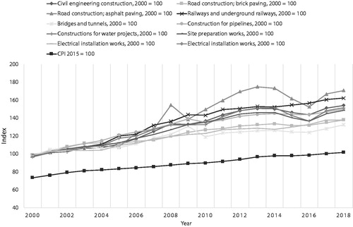
Table 2. Long-term differential inflation rates and their impact on discounting.

	1	2	3	4	5	6	7	8	9
Total inflation	2.6%	1.9%	3.1%	2.8%	1.7%	2.3%	2.5%	2.3%	1.9%
General inflation	1.8%	1.8%	1.8%	1.8%	1.8%	1.8%	1.8%	1.8%	1.8%
Differential inflation	0.7%	0.0%	1.3%	1.0%	−0.2%	0.5%	0.7%	0.4%	0.1%
Real discount rate A	5.0%	5.0%	5.0%	5.0%	5.0%	5.0%	5.0%	5.0%	5.0%
Net discount rate A	4.2%	5.0%	3.7%	4.0%	5.2%	4.5%	4.3%	4.5%	4.9%
Deviation for A	15.2%	0.7%	26.9%	20.6%	−3.4%	10.6%	14.2%	9.3%	1.5%
Real discount rate B	3.0%	3.0%	3.0%	3.0%	3.0%	3.0%	3.0%	3.0%	3.0%
Net discount rate B	2.3%	3.0%	1.7%	2.0%	3.2%	2.5%	2.3%	2.5%	2.9%
Deviation for B	24.8%	1.1%	44.0%	33.7%	−5.5%	17.4%	23.3%	15.3%	2.5%

1. Civil engineering construction (weighted average).

2. Road construction; brick paving.

3. Road construction; asphalt paving.

4. Railways and underground railways.

5. Bridges and tunnels.

6. Construction of pipelines.

7. Construction for water projects.

8. Site preparation works.

9. Electrical installation works.

The top part of Table 2 shows the total inflation rates, general inflation rates and differential inflation rates for nine aggregated civil engineering cost components. The magnitude of the differential inflation rates ranges from −0.2% to 1.3% for these data sets.

In the Netherlands, public sector organizations use real discount rates between 3% and 5%. The middle part of Table 2 shows the impact of the differential inflation rates on net discounting for an organization A that uses a real discount rate of 5%. The impact of differential inflation on discounting follows the ratio: $(1+d)/(1+r)=1/(1+r_{\mathit{net}}),$ where $r_{\mathit{net}}$ = net discount rate in real terms (opposed to nominal). For organization A, differential inflation changes the effective real discount rate from 5% to a range of 3.7% to 5.2%. This results in deviations from the real discount rate from −3.4% to 26.9%. The deviation is calculated by $1-r_{\mathit{net}}/r.$

The bottom part of Table 2 shows the same analysis for organization B which uses a real discount rate of 3%. In this situation, the net discount rate ranges between 1.7% and 3.2% and the deviations from the real discount range between -5.5% and 44%.

From the analysis, two conclusions are drawn. First, the differential inflation rates between cost components differ and can be positive or negative values. Second, for organizations that use low real discount rates, this differential inflation can significantly affect the net discounting in present value calculations. Present value calculations are known to be sensitive to changes in discount rates. Therefore, the presence of differential inflation should be carefully assessed.

The analysis is conducted with publicly available aggregated data that levels off values for specific subgroups and the impact of local circumstances. This type of aggregated data should be used with caution. Non-aggregated data fitting local circumstances are also available but not publicly published because this information is often confidential or competitive.

Although not similar in objective, a UK study on the development of construction output prices illustrates the significance of inflationary effects in UK construction industry (Yu and Ive 2011). A study by Mirzadeh et al. (2014) emphasize a proper assessment of differential inflation rates reflecting specific circumstances. This study provides a model for such assessment for road infrastructure in Sweden.

Research method

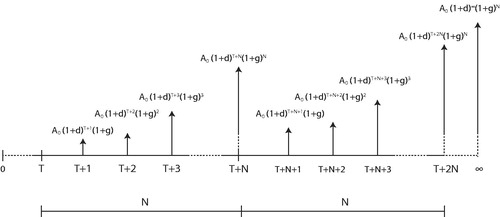
The previous section demonstrates differential inflation and how it affects the net discounting in present value calculations. Classic replacement analysis techniques cannot handle differential inflation because differential inflation undermines the repeatability assumption of the challenger’s cash flows. Therefore, the approach to infrastructure replacement analysis under differential inflation is based on the capitalized equivalent approach with adjustments to ageing and differential inflation.

The capitalized equivalent approach compares the present values of defender-challenger replacement scenarios over an infinite time horizon. For a cost model: let $T$ be the time for replacing the defender in number of years starting from zero, then, the objective is to identify the value of $T^{\mathrm{*}}$ that minimises the total present value of the combined keep-replace scenarios according to Equation 3(3) $$\underset{}{P^{*}}=\underset{T}{\min }\left(\sum _{i=0}^T\frac{F_i}{{(1+r)}^i}+\sum _{k=T}^{\infty }\frac{F_k}{{(1+r)}^k}\right),$$(3) . (3) $$\underset{}{P^{*}}=\underset{T}{\min }\left(\sum _{i=0}^T\frac{F_i}{{(1+r)}^i}+\sum _{k=T}^{\infty }\frac{F_k}{{(1+r)}^k}\right),$$(3) where $P^{\mathrm{*}}$ = minimum present value of a keep-replace scenario over an infinite time horizon; $F_i$ = real cash flow of the defender in year $i;$ $F_k$ = real cash flow of the challenger(s) in year $k,$ $T$ = year of replacement of a defender relative to starting year zero and $r$ = real interest rate.

The following sections derive generic mathematical relationships to perform the present value calculations for different types of life cycle activities subject to ageing and differential inflation for the defender and challenger. Combining these mathematical equations allows for a relatively compact spreadsheet calculation as opposed to complex DP-modelling, which will be used for comparison. The restrictions of this approach are twofold. First, this approach assumes, the inflation adjusted perpetuity of the first challenger’s cashflows is a suitable approximation of all future cash flows.

The second restriction is the assumption that the economic life of the challenger remains unchanged when evaluated in the future and is approximated by its forecasted functional life. Differential inflation can cause changes in economic lives when evaluated on future dates. However, because of high investment costs and relatively low operational expenditures combined with long functional lives (e.g. 100 years), the potential impact of changing economic lives is not differential for determining the optimal first replacement time, which is demonstrated in the case study.

Life cycle activities consist of investments, major overhauls and operation and maintenance (O&M) expenditures. For the capitalized equivalent approach, the cumulative cash flows of the defender are combined with the perpetuities of the challenger’s cash flows. In the following paragraphs, formulae are derived including differential inflation and ageing for both the defender and challenger. For readability, differential inflation $\left(d\right),$ ageing $\left(g\right)$ and interval $\left(n\right)$ are not indexed for specific cost components in the generic derivations. In the specific application of the formulae, different cost components will have different values for differential inflation, ageing and intervals.

Cumulative present values of the defender’s cash flows subject to differential inflation and ageing

The cash flows of the defender generally consist of an initial renovation, intermediate major overhauls and yearly O&M costs. The defender is replaced by a challenger at a future time $T$ relative to year zero. Potential salvage values, scrap and demolition values of a defender are considered part of the investment costs of the challenger.

Present values of the defender’s major overhauls subject to differential inflation

The cumulative present values of the initial renovation and major overhauls of a defender follow traditional discounting. The cash flows of the renovation and major overhauls are inflated with differential inflation and discounted using a real discount rate. In general, major overhauls are not subject to ageing; however, ageing can be included in the cash flows if required.

For example, the present value of a defender’s major overhaul with a current price level $M_0,$ starting at time $t\le T,$ with an interval $n,$ which is repeated $z$ times within period $\left[t,T\right]$ with $t+\mathit{zn}\le T$ is calculated as Equation 4(4) $$P_D^M{[0,T]}_t=\hspace{0.17em}{M}_0{\left(\frac{1+d}{1+r}\right)}^t+M_0{\left(\frac{1+d}{1+r}\right)}^{t+n}+M_0{\left(\frac{1+d}{1+r}\right)}^{t+2n}+\dots +M_0{\left(\frac{1+d}{1+r}\right)}^{t+\mathit{zn}}.$$(4) . (4) $$P_D^M{[0,T]}_t=\hspace{0.17em}{M}_0{\left(\frac{1+d}{1+r}\right)}^t+M_0{\left(\frac{1+d}{1+r}\right)}^{t+n}+M_0{\left(\frac{1+d}{1+r}\right)}^{t+2n}+\dots +M_0{\left(\frac{1+d}{1+r}\right)}^{t+\mathit{zn}}.$$(4)

Including ageing with a yearly percentage growth of $g$ would require substituting $\left(1+d\right)$ with $\left(1+d\right)\left(1+g\right).$

Present values of defender’s annuities subject to differential inflation and ageing

More interesting is the calculation of the cumulative present values of the regular yearly O&M expenditures due to different possibilities of ageing and differential inflation. Three situations are noted: operation expenditures are an annuity subject to (1) differential inflation only, (2) ageing only and (3) ageing and differential inflation. The engineering economics toolbox provides the standard geometric gradient series formula for discrete compounding (Park 2011), which is adapted to include differential inflation and ageing. This standard formula calculates the present value of an annuity starting at year 1, growing with $x\mathrm{\%}$ per year, and is given by Equation 5(5) $$P{[0,T]}_1=A_0(1+x)\cdot \frac{1-{\left(\frac{1+x}{1+r}\right)}^T}{r-x}\forall x\ne r,$$(5) . (5) $$P{[0,T]}_1=A_0(1+x)\cdot \frac{1-{\left(\frac{1+x}{1+r}\right)}^T}{r-x}\forall x\ne r,$$(5) with $P[0,T]$= present value at $t\mathrm{ }=\mathrm{ }0$ of an annuity starting at year 1 and ending in year $T;$ $A_0$ = year zero price level of the annuity; $x$ = the percentage of yearly growth; $A_0\left(1+x\right)$ = the first year cost of the annuity; and $r$ = the real discount rate.

The percentage of yearly growth $x$ in Equation 5(5) $$P{[0,T]}_1=A_0(1+x)\cdot \frac{1-{\left(\frac{1+x}{1+r}\right)}^T}{r-x}\forall x\ne r,$$(5) can be substituted with differential inflation $d$ or ageing $g.$ However, including both differential inflation $d$ and ageing $g$ simultaneously requires substituting $\left(1+x\right)$ with $\left(1+d\right)\left(1+g\right)$ and consequently:$\mathrm{ }x=\left(1+d\right)\left(1+g\right)-1.$

Performing these substitutions results in the following relationship (Equation 6(6) $$P_D^A{[0,T]}_1=A_0(1+d)(1+g)\cdot \frac{1-{\left(\frac{(1+d)(1+g)}{1+r}\right)}^T}{r-(1+d)(1+g)+1},$$(6) ) to calculate the present value of a defender’s annuity over time $[0,T],$ subject to both differential inflation and ageing: (6) $$P_D^A{[0,T]}_1=A_0(1+d)(1+g)\cdot \frac{1-{\left(\frac{(1+d)(1+g)}{1+r}\right)}^T}{r-(1+d)(1+g)+1},$$(6) with $P_D^A{\left[0,T\right]}_1$= present value of a defender’s annuity starting at year 1 and ending in year $T;$ $A_0$ = year zero price level of the annuity; $d$ = differential inflation; $g$ = yearly growth percentage for ageing; $A_0\left(1+d\right)\left(1+g\right)$ = first year cost of the annuity; and $r$ = the real discount rate.

With generic Equations 4 and 6(6) $$P_D^A{[0,T]}_1=A_0(1+d)(1+g)\cdot \frac{1-{\left(\frac{(1+d)(1+g)}{1+r}\right)}^T}{r-(1+d)(1+g)+1},$$(6) , the present values of the cash flows of a defender in time interval $\left[0,T\right]$ are calculated. The following section develops mathematical equations to calculate the present values of the challenger’s cash flows occurring in interval $\left[T,\mathrm{\infty }\right].$

Present values of the challenger’s perpetual cash flows subject to differential inflation and ageing

This section develops equations to calculate the present values ($t=0$) of the cash flows of the challenger $P_C\mathrm{ }{\left[0,\mathrm{\infty }\right]}_T$ for cash flows occurring in interval $\left[T,\mathrm{\infty }\right].$ The challenger is installed at time $T$ and perpetually replaced over its life cycle $N.$

Present values of the challenger’s perpetual investment and major overhauls costs

Activities such as the initial investment and major overhauls are perpetuities with intervals of $N$ and $n,$ respectively, and are generally subject to differential inflation only. In exceptional cases, major overhauls may also be subject to ageing. However, in these cases, it is easier to consider the ageing major overhauls as different activities with their own repeating intervals than to derive a mathematical equation that includes differential inflation and ageing.

The cash flows of a perpetuity of the initial investment $I_0$ (price level year 0) starting at time $T$ relative to start year zero, with interval $N$ and subject to differential inflation $d,$ are depicted in Figure 2.

Figure 2. Cash flows of a perpetuity of investment $I_0$ with interval $N,$ starting at time $T$ and subject to differential inflation.

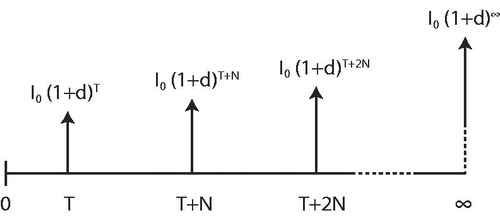
The present value of this challenger’s investment perpetuity is given by straightforward discounting as in Equation 7(7) $$P_C^I{[0,\infty ]}_T={\left(\frac{1}{1+r}\right)}^T\cdot (I_0{(1+d)}^T+I_0{(1+d)}^T{(\frac{1+d}{1+r})}^N+I_0{(1+d)}^T{(\frac{1+d}{1+r})}^{2N}+\dots .),$$(7) . (7) $$P_C^I{[0,\infty ]}_T={\left(\frac{1}{1+r}\right)}^T\cdot (I_0{(1+d)}^T+I_0{(1+d)}^T{(\frac{1+d}{1+r})}^N+I_0{(1+d)}^T{(\frac{1+d}{1+r})}^{2N}+\dots .),$$(7) where $P_C^I{\left[0,\mathrm{\infty }\right]}_T$ = the present value at $t=0$ of a perpetuity of the challenger’s investment; $I_0$ is the cost of the investment at price level 0; $T$ is the start time of the investment; $N$ is the interval of the investment; $d$ is the differential inflation specific for this investment; and $r$ is the real interest rate.

The coefficients in Equation 7(7) $$P_C^I{[0,\infty ]}_T={\left(\frac{1}{1+r}\right)}^T\cdot (I_0{(1+d)}^T+I_0{(1+d)}^T{(\frac{1+d}{1+r})}^N+I_0{(1+d)}^T{(\frac{1+d}{1+r})}^{2N}+\dots .),$$(7) are a geometric series. Therefore, Equation 7(7) $$P_C^I{[0,\infty ]}_T={\left(\frac{1}{1+r}\right)}^T\cdot (I_0{(1+d)}^T+I_0{(1+d)}^T{(\frac{1+d}{1+r})}^N+I_0{(1+d)}^T{(\frac{1+d}{1+r})}^{2N}+\dots .),$$(7) can be rewritten as Equation 8(8) $$P_C^I{[0,\infty ]}_T=I_0\cdot \frac{{\left(\frac{1+d}{1+r}\right)}^T}{1-{\left(\frac{1+d}{1+r}\right)}^N}.$$(8) . (8) $$P_C^I{[0,\infty ]}_T=I_0\cdot \frac{{\left(\frac{1+d}{1+r}\right)}^T}{1-{\left(\frac{1+d}{1+r}\right)}^N}.$$(8)

Let: (9) $$K=\left(\frac{1+d}{1+r}\right),$$(9)

Then, Equation 8(8) $$P_C^I{[0,\infty ]}_T=I_0\cdot \frac{{\left(\frac{1+d}{1+r}\right)}^T}{1-{\left(\frac{1+d}{1+r}\right)}^N}.$$(8) simplifies to Equation 10(10) $$P_C^I{[0,\infty ]}_T=I_0\cdot \frac{K^T}{1-K^N}.$$(10) . (10) $$P_C^I{[0,\infty ]}_T=I_0\cdot \frac{K^T}{1-K^N}.$$(10)

Summarizing: Equation 10(10) $$P_C^I{[0,\infty ]}_T=I_0\cdot \frac{K^T}{1-K^N}.$$(10) calculates the present value at $t=0$ of an investment starting at time $T,$ repeating itself with an interval $N$ and subject to differential inflation $d.$

For the present values of a perpetuity of a major overhaul, two situations are considered. The first and most common situation is the interval $n$ of the major overhaul is a common multiple in the functional life $N$ of the challenger, for example $n\mathrm{ }=\mathrm{ }20\mathrm{ }\mathrm{years}$ and $N\mathrm{ }=\mathrm{ }100\mathrm{ }\mathrm{years}.$ In that case, the present value of a major overhaul $M_0$ starting at year $t=T+n,$ with an interval $n$ is calculated similar to the perpetuity of the investment. Additionally, a perpetuity of this major overhaul with interval $N$ starting at time $T+N$ (time of second investment) needs to be subtracted to prevent the simultaneous occurrence of a major overhaul with successive investments. Hence, a challenger’s present value with major overhauls starting at $t\mathrm{ }=\mathrm{ }T+n,$ with an interval $n$ that is a common multiple in the challenger’s functional life $N,$ is computed by Equation 11(11) $$P_C^M{[0,\infty ]}_{T+n}=M_0\cdot \left(\frac{K^{T+n}}{1-K^n}-\frac{K^{T+N}}{1-K^N}\right).$$(11) . (11) $$P_C^M{[0,\infty ]}_{T+n}=M_0\cdot \left(\frac{K^{T+n}}{1-K^n}-\frac{K^{T+N}}{1-K^N}\right).$$(11)

For the readers’ convenience, $K$ as defined in Equation 9(9) $$K=\left(\frac{1+d}{1+r}\right),$$(9) is not substituted with another symbol in Equation 11(11) $$P_C^M{[0,\infty ]}_{T+n}=M_0\cdot \left(\frac{K^{T+n}}{1-K^n}-\frac{K^{T+N}}{1-K^N}\right).$$(11) . However, in the application of the formula, the value of $K$ depends on the specific differential inflation of a cost component.

The second situation, which is less common, encompasses major overhauls with an interval $n$ that is not a common multiple in the challenger’s functional life $N.$ For example, $N\mathrm{ }=\mathrm{ }100\mathrm{ }\mathrm{years}$ and $n\mathrm{ }=\mathrm{ }40\mathrm{ }\mathrm{years}.$ Interval $n$ may not be stationary. The approach in this situation is to calculate the relative present value $P_C^M{\left[T,T+N\right]}_{T+n}$ at time T of the major overhauls occurring in the first challenger’s life cycle (analogous to Equation 4) and treat this value as a perpetuity starting at time $T$ with interval $N,$ such as investment $I_0,$ thus, analogous to Equation 10(10) $$P_C^I{[0,\infty ]}_T=I_0\cdot \frac{K^T}{1-K^N}.$$(10) . Consequently, the challenger’s present value with major overhauls with an interval $n$ that is not a common multiple in the functional life $N$ is computed by Equation 12(12) $$P_C^M{[0,\infty ]}_{T+n}=P_C^M{[T,T+N]}_{T+n}\cdot \left(\frac{K^T}{1-K^N}\right).$$(12) . (12) $$P_C^M{[0,\infty ]}_{T+n}=P_C^M{[T,T+N]}_{T+n}\cdot \left(\frac{K^T}{1-K^N}\right).$$(12)

Present values of perpetuities of the challenger’s yearly operational expenditures

Operational expenditures of the challenger are modelled as yearly costs A₀ (price level year 0), starting at year $t\mathrm{\hspace{0.17em}}=T+1,$ and grow each year with a factor. Again, three situations are considered: (1) differential inflation only, (2) ageing only or (3) differential inflation and ageing. In contrast to the approach followed for the defender, differential inflation and ageing cannot be treated similarly for the challenger’s operational perpetuities. This finding is illustrated in the cash flow diagrams in Figures 3, 4 and 5, which depict the situations for differential inflation only, ageing only and differential inflation and ageing, respectively.

Figure 3. Cash flows of a perpetuity of an annuity starting at year $t=T+1$ and subject to differential inflation $d.$

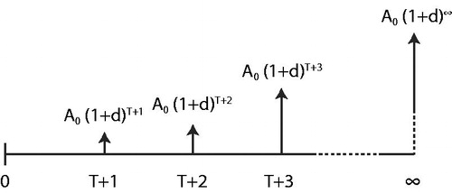
Figure 4. Cash flows of a perpetuity of an annuity starting at year $t=T+1$ and subject to ageing.

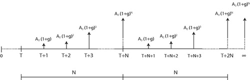
Figure 5. Cash flows of a perpetuity of an annuity starting at year $t=T+1$ and subject to differential inflation and ageing.

Considering differential inflation only

The calculation of the present value of a perpetuity of yearly expenditures subject to only differential inflation follows the same approach as Equation 10(10) $$P_C^I{[0,\infty ]}_T=I_0\cdot \frac{K^T}{1-K^N}.$$(10) . Operational expenditures are a perpetuity with an interval of $n=1$ and subject to differential inflation. The cash flows are depicted in Figure 3.

The present value of a perpetuity of yearly operational expenditures starting at year $t\mathrm{\hspace{0.17em}}=\mathrm{ }T+1$ and subject to only differential inflation $d$ follows from Equation 13(13) $$P_C^{A,\hspace{0.17em}d\hspace{0.17em}\mathit{only}}{[0,\infty ]}_{T+1}=A_0\cdot \frac{K^{T+1}}{1-K}.$$(13) . (13) $$P_C^{A,\hspace{0.17em}d\hspace{0.17em}\mathit{only}}{[0,\infty ]}_{T+1}=A_0\cdot \frac{K^{T+1}}{1-K}.$$(13)

Considering ageing only

The second case concerns an operational activity subject to only ageing (no differential inflation) due to increasing corrective maintenance. The calculation of the present value of the perpetuity follows a different approach. After replacement of the challenger, the corrective maintenance expenditures will start at their first-year level again. The cash flows are depicted in Figure 4. $N$ is the life cycle of the challenger, installed at time $T,$ and $t\mathrm{ }=\mathrm{ }T+1$ are the first year of the annual cost.

The relative present value of yearly expenditures subject to ageing over one life cycle $N$ of a challenger is independent of the challenger’s start time $T.$ The first-year costs for ageing will always be $A_0\left(1+g\right).$ Therefore, the relative present value of a challenger’s annuity subject to only ageing follows directly from Equation 8(8) $$P_C^I{[0,\infty ]}_T=I_0\cdot \frac{{\left(\frac{1+d}{1+r}\right)}^T}{1-{\left(\frac{1+d}{1+r}\right)}^N}.$$(8) , where $x$ is substituted with the ageing growth factor $g$ and is given by Equation 14(14) $$P_C^{A,\hspace{0.17em}g\hspace{0.17em}\mathit{only}}{[T,T+N]}_{T+1}=A_{{}_0}(1+g)\frac{1-{\left(\frac{1+g}{1+r}\right)}^N}{r-g}.$$(14) . (14) $$P_C^{A,\hspace{0.17em}g\hspace{0.17em}\mathit{only}}{[T,T+N]}_{T+1}=A_{{}_0}(1+g)\frac{1-{\left(\frac{1+g}{1+r}\right)}^N}{r-g}.$$(14)

$P_C^{A,\mathrm{ }g\mathrm{ }\mathit{only}}{\left[T,T+N\right]}_{T+1}$ is a relative present value at time $T$ of annuities subject to ageing over life cycle $N.$ This relative present value will repeat itself with an interval $N$ (the challenger’s life cycle). In accordance with the approach of Equation 8(8) $$P_C^I{[0,\infty ]}_T=I_0\cdot \frac{{\left(\frac{1+d}{1+r}\right)}^T}{1-{\left(\frac{1+d}{1+r}\right)}^N}.$$(8) with $d=0,$ the present value of its perpetuity for only ageing (without differential inflation) becomes Equation 15(15) $$P_C^{A,\hspace{0.17em}g\hspace{0.17em}\mathit{only}}{[0,\infty ]}_{T+1}= P_C^{A,\hspace{0.17em}g\hspace{0.17em}\mathit{only}}{[T,T+N]}_{T+1}\cdot \frac{{\left(\frac{1}{1+r}\right)}^T}{1-{\left(\frac{1}{1+r}\right)}^N}=A_{{}_0}(1+g)\frac{{\left(\frac{1}{1+r}\right)}^T}{r-g}$$(15) . (15) $$P_C^{A,\hspace{0.17em}g\hspace{0.17em}\mathit{only}}{[0,\infty ]}_{T+1}= P_C^{A,\hspace{0.17em}g\hspace{0.17em}\mathit{only}}{[T,T+N]}_{T+1}\cdot \frac{{\left(\frac{1}{1+r}\right)}^T}{1-{\left(\frac{1}{1+r}\right)}^N}=A_{{}_0}(1+g)\frac{{\left(\frac{1}{1+r}\right)}^T}{r-g}$$(15)

Equation 15(15) $$P_C^{A,\hspace{0.17em}g\hspace{0.17em}\mathit{only}}{[0,\infty ]}_{T+1}= P_C^{A,\hspace{0.17em}g\hspace{0.17em}\mathit{only}}{[T,T+N]}_{T+1}\cdot \frac{{\left(\frac{1}{1+r}\right)}^T}{1-{\left(\frac{1}{1+r}\right)}^N}=A_{{}_0}(1+g)\frac{{\left(\frac{1}{1+r}\right)}^T}{r-g}$$(15) calculates the present value at $t=0$ of the challenger’s perpetuity of yearly operational costs, starting at time $T+1,$ subject to only ageing.

Ageing and differential inflation

The third case concerns yearly operational expenditures subject to differential inflation and ageing. The cash flows are shown in Figure 5. The approach is to calculate the current present value of an annuity subject to differential inflation and ageing over one life cycle $N,$ assuming an immediate instalment of the challenger. This present value is calculated with Equation 6(6) $$P_D^A{[0,T]}_1=A_0(1+d)(1+g)\cdot \frac{1-{\left(\frac{(1+d)(1+g)}{1+r}\right)}^T}{r-(1+d)(1+g)+1},$$(6) . Second, the present value is considered an infinite repetitive activity with interval $N,$ which can start at any time $T$ and is subject to differential inflation, analogous to the calculation of the perpetuity of the investment in Equation 8(8) $$P_C^I{[0,\infty ]}_T=I_0\cdot \frac{{\left(\frac{1+d}{1+r}\right)}^T}{1-{\left(\frac{1+d}{1+r}\right)}^N}.$$(8) .

The present value of the first life cycle of cash flows occurring over period $N$ for an annuity subject to differential inflation and ageing is calculated as Equation 16(16) $$P_C^{A,\hspace{0.17em}d\hspace{0.17em}\&\hspace{0.17em}g}{[0,N]}_1= A_{{}_0}(1+d)(1+g)\cdot \left(\frac{1-{\left(\frac{(1+d)(1+g)}{1+r}\right)}^N}{r-(1+d)(1+g)+1}\right).$$(16) (analogous to Equation 6(6) $$P_D^A{[0,T]}_1=A_0(1+d)(1+g)\cdot \frac{1-{\left(\frac{(1+d)(1+g)}{1+r}\right)}^T}{r-(1+d)(1+g)+1},$$(6) ). (16) $$P_C^{A,\hspace{0.17em}d\hspace{0.17em}\&\hspace{0.17em}g}{[0,N]}_1= A_{{}_0}(1+d)(1+g)\cdot \left(\frac{1-{\left(\frac{(1+d)(1+g)}{1+r}\right)}^N}{r-(1+d)(1+g)+1}\right).$$(16)

The present value (at $t\mathrm{\hspace{0.17em}}=\mathrm{\hspace{0.17em}}0$) of its perpetuity with interval $N,$ starting at an arbitrary time $T+1$ and subject to differential inflation, is calculated as Equation 17(17) $$P_C^{A,d\hspace{0.17em}\&\hspace{0.17em}g}{[0,\infty ]}_{T+1}= A_{{}_0}(1+d)(1+g)\cdot \left(\frac{1-{\left(\frac{(1+d)(1+g)}{1+r}\right)}^N}{r-(1+d)(1+g)+1}\right)\cdot \left(\frac{{\left(\frac{1+d}{1+r}\right)}^T}{1-{\left(\frac{1+d}{1+r}\right)}^N}\right).$$(17) . (17) $$P_C^{A,d\hspace{0.17em}\&\hspace{0.17em}g}{[0,\infty ]}_{T+1}= A_{{}_0}(1+d)(1+g)\cdot \left(\frac{1-{\left(\frac{(1+d)(1+g)}{1+r}\right)}^N}{r-(1+d)(1+g)+1}\right)\cdot \left(\frac{{\left(\frac{1+d}{1+r}\right)}^T}{1-{\left(\frac{1+d}{1+r}\right)}^N}\right).$$(17)

The last expression in Equation 17(17) $$P_C^{A,d\hspace{0.17em}\&\hspace{0.17em}g}{[0,\infty ]}_{T+1}= A_{{}_0}(1+d)(1+g)\cdot \left(\frac{1-{\left(\frac{(1+d)(1+g)}{1+r}\right)}^N}{r-(1+d)(1+g)+1}\right)\cdot \left(\frac{{\left(\frac{1+d}{1+r}\right)}^T}{1-{\left(\frac{1+d}{1+r}\right)}^N}\right).$$(17) represents the differential inflation when a challenger is installed at time $T$ instead of time zero. Using the same notation, Equation 17(17) $$P_C^{A,d\hspace{0.17em}\&\hspace{0.17em}g}{[0,\infty ]}_{T+1}= A_{{}_0}(1+d)(1+g)\cdot \left(\frac{1-{\left(\frac{(1+d)(1+g)}{1+r}\right)}^N}{r-(1+d)(1+g)+1}\right)\cdot \left(\frac{{\left(\frac{1+d}{1+r}\right)}^T}{1-{\left(\frac{1+d}{1+r}\right)}^N}\right).$$(17) can be simplified to Equation 18(18) $$P_C^{A,\hspace{0.17em}d\hspace{0.17em}\&\hspace{0.17em}g}{[0,\infty ]}_{T+1}=P_C^{A,\hspace{0.17em}d\hspace{0.17em}\&\hspace{0.17em}g}{[0,N]}_1\cdot \frac{K^T}{1-K^N}.$$(18) . (18) $$P_C^{A,\hspace{0.17em}d\hspace{0.17em}\&\hspace{0.17em}g}{[0,\infty ]}_{T+1}=P_C^{A,\hspace{0.17em}d\hspace{0.17em}\&\hspace{0.17em}g}{[0,N]}_1\cdot \frac{K^T}{1-K^N}.$$(18)

Equation 17(17) $$P_C^{A,d\hspace{0.17em}\&\hspace{0.17em}g}{[0,\infty ]}_{T+1}= A_{{}_0}(1+d)(1+g)\cdot \left(\frac{1-{\left(\frac{(1+d)(1+g)}{1+r}\right)}^N}{r-(1+d)(1+g)+1}\right)\cdot \left(\frac{{\left(\frac{1+d}{1+r}\right)}^T}{1-{\left(\frac{1+d}{1+r}\right)}^N}\right).$$(17) is generic for the three situations of differential inflation only, ageing only and differential and ageing. Setting $d$ or $g$ equal to zero and making proper substitutions results in Equations 13(13) $$P_C^{A,\hspace{0.17em}d\hspace{0.17em}\mathit{only}}{[0,\infty ]}_{T+1}=A_0\cdot \frac{K^{T+1}}{1-K}.$$(13) and 15(15) $$P_C^{A,\hspace{0.17em}g\hspace{0.17em}\mathit{only}}{[0,\infty ]}_{T+1}= P_C^{A,\hspace{0.17em}g\hspace{0.17em}\mathit{only}}{[T,T+N]}_{T+1}\cdot \frac{{\left(\frac{1}{1+r}\right)}^T}{1-{\left(\frac{1}{1+r}\right)}^N}=A_{{}_0}(1+g)\frac{{\left(\frac{1}{1+r}\right)}^T}{r-g}$$(15) , respectively.

The formulae for calculating the present values of the defender and challenger subject to ageing and differential inflation are combined in the capitalized equivalent approach. The proper substitutions are verified by discounting forecasted cash flows subject to differential inflation and age-related growth on a time horizon that approximates infinity. Forecasting cash flows subject to differential inflation and ageing for all combined keep-replace scenarios is much more time consuming and prone to mistakes.

Demonstration of an inflation adjusted capitalized equivalent replacement analysis

For demonstration of the method, an existing case study in the Netherlands is used, a steel bridge owned by a governmental organization. Based on the current condition, the expected maximum useful life is 35 years after a thorough and expensive renovation, including reinforcement. If replaced, the bridge will be replaced by a concrete bridge with an expected useful life of 100 years. The asset owner is interested in the optimal replacement time of the existing bridge for several reasons.

First, the immediate decision for a renovation or replacement is justified. Second, the current bridge is part of a larger asset portfolio. The analysis directly contributes to the long-term capital investment planning and the required budget forecasts. Moreover, the analysis is directly applicable to other bridges in the asset portfolio. Only changes of input values are required.

Data

The cost estimates are provided by the asset owner (Table 3) and proportionally adjusted for confidentiality. This proportional adjustment does not affect the interpretation of results and the presented cost values could be valid for another situation.

Table 3. Data for defender – challenger analysis under differential inflation and ageing.

	Start year first cycle (year)	Interval $n\mathrm{ }$(year)	Ageing $g\mathrm{ }$(%/year)	Differential inflation $d\mathrm{ }$(%/year)	Costs in price level year 0^a (€)
Defender
Renovation	0	–	–	–	€ 3,000,000
O&M	1	1	0.50%	0.85%	€ 26,250
Major overhauls steel	10	20	–	0.96%	€ 1,500,000
Major overhauls concrete	20	20	–	0.80%	€ 425,000
Major overhauls asphalt	10	10	–	1.44%	€ 62,500
Challenger
Investment	0	100	–	0.12%	€ 8,300,000
O&M	1	1	0.20%	0.85%	€ 7,500
Major overhauls steel	20	20	–	0.96%	€ 178,750
Major overhauls concrete	20	20	–	0.80%	€ 175,000
Major overhauls asphalt	10	10	–	1.44%	€ 62,500

^aCosts begin at start year of a cycle and repeat with interval $n.$

The estimates for differential inflation rates are obtained from analyzing specific producer price indices (PPI) and the consumer price index (CPI) from 1995 to 2017. The publicly available CPI data is found in the data disclosure statement at the end of this paper. The raw PPI data used for this case study is obtained from a specialized knowledge centre (CROW 2018).

The average yearly general inflation rate over this period, 1.87%, is derived from the CPI. The slight difference in general inflation rate, in comparison with the illustrative analysis in the section on differential inflation, is caused by a more extensive data set from the same source that allows for a longer analysis period. Due to the long-life cycles of infrastructure assets, preference goes to the longest period available.

The total inflation for different cost components in the case study is in consultation with the asset owner, derived from the respective PPI’s and proportionally combined in baskets where appropriate (e.g. a combination of labour and materials). The values deviate from the values in the section on differential inflation because other cost groups are analyzed, and less aggregated data are used. Equation 1(1) $$d=\mathrm{ }\frac{f_{\mathit{tot}}-f}{1+f}$$(1) is used to calculate the differential inflation, as depicted in Table 3.

The estimates for cost development as a consequence of ageing are made in consultation with cost and maintenance engineers.

Calculation

First, the economic life of the challenger as if installed today is calculated as explained in the literature on engineering economics (Park 2011, Sullivan et al. 2012, Hastings 2015, Newnan et al. 2016), which results in $N^{\mathrm{*}}=N=100$ years with an ${\mathit{EAC}}_C^{\mathrm{*}}\mathrm{ }\left(t=0\right)$ of €448,910. Currently, the economic life is bounded by the challenger’s functional life $N.$

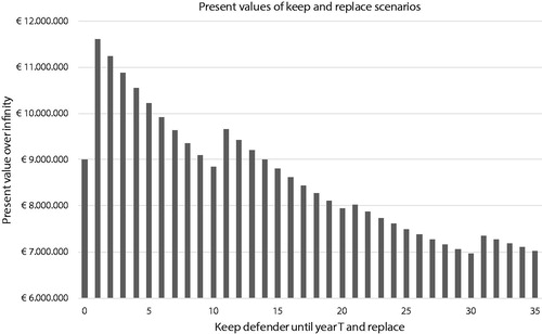
Under the assumption the challenger’s future life cycle costs are a perpetuity with interval $N,$ the defender-challenger analysis is reduced to a spreadsheet calculation using the derived formulae. The combined present values for the 35 keep-replace scenarios are depicted in Figure 6 and Supplemental material, Appendix B, Table B1. The results of underlying calculations (including equations used) for the defender and challenger are presented in Supplemental material, Appendix B, Appendix B and B3.

Figure 6. Present values for keep-replace scenarios subject to differential inflation and ageing.

Analysis of results

The spikes in Figure 6 are caused by the defender’s major overhauls. The lowest present value occurs for scenario 30; keeping the defender for 30 years and replacing the defender at the end of the 30th year, immediately before the defender’s planned major overhaul. However, more conclusions can be derived. For example, the defender’s renovation is only sensible if the defender can be kept in service for at least another 10 years, until then, there is no financial gain.

If an asset owner is not certain about a functional life exceeding 10 years, and the preferable 15 years in this case study, the best option may be to replace the defender immediately. Similarly, replacing the defender in year 30 is the cheapest option because its useful life is bounded by 35 years. However, if there is reason to believe the remaining life of the defender exceeds 35 years, the calculations should be extended to incorporate more maintain-replace scenarios. A graph such as Figure 6 supports a decision maker constructing motivated short- and long-term capital investment planning.

As discussed in the literature review, a classic capitalized equivalent analysis ignores differential inflation. This analysis is quickly simulated by letting the values for differential inflation be approximately zero in the inflation adjusted model. For the case study, this results in an optimal replacement in year 35 instead of year 30. Differential inflation makes the concrete replacement option more attractive and the steel defender less attractive, which is motivated by the relative high differential inflation rate for steel and the defender’s expensive major overhauls for steel.

Practical implications

From a practical point of view, a replacement decision in 30 years or 35 years may not seem of immediate interest. This, however, is also an answer to the question of this authority. Although a concrete bridge is cheaper in maintenance, replacing it for that reason would economically not be a wise decision in this case study. From a life cycle costs point of view, it is better to invest in a renovation and to incur the higher maintenance costs of the current steel bridge for at least another 10 and preferably 30 years.

Another practical use of this replacement optimization method is that this bridge is not a stand-alone case. This authority owns over thousand bridges. Most were built around 1960–1970 and since then subject to increasing traffic intensity. Inspection and structural safety assessments determine the useful remaining life. The economic optimization method efficiently determines the economic remaining life of an existing asset which is less than or bounded by its useful life. Moreover, this method accounts for differential inflation, which grows in importance because of the low discount rates used by public sector organizations. This method directly supports the long-term capital investment planning of infrastructure in a fast and efficient manner. In this context, the current research shows that ignoring differential inflation will lead to a less accurate estimate of the long-term capital investment planning.

In general, low discount rates and long lives stress the importance of a careful assessment of the presence and impact of differential inflation. Historic PPI data are publicly available at, for example, a bureau of labour statistics. The developed formulae allow a rapid inclusion of differential inflation in a common defender-challenger replacement challenge. This research provides a pragmatic alternative to classic approaches that cannot handle inflation and case-specific DP-modelling. The inflation adjusted capitalized equivalent approach will by definition provide more accurate results than the classic capitalized equivalent approach. The assumption of a challenger’s constant life $\mathrm{N}$ underlies both approaches. The developed inflation adjusted capitalised equivalent approach also easily accounts for ageing, which can be modelled with an underlying stochastic process. Mathematically, the application of the method is comparable to classic approaches.

Comparison with DP-solution

The DP-solution to this defender-challenger problem relaxes the assumption of a constant challenger’s $N$ since it optimises the entire challenger’s replacement chain, including future economic lives. The approach of Wagner (1975) is used for comparison with the approach developed in the current research. Wagner’s approach is explained in Supplemental material, Appendix A.

A disadvantage of a DP-solution is that an infinite calculation horizon is approximated by a bounded calculation horizon, sufficiently long to capture the future cash flows that contribute to the total present value (Wagner 1975; Regnier et al. 2004). The difficulty of applying the DP-solution to an approximated infinite calculation horizon is the size of the solution space, which is reflected in a cost matrix that contains all possible keep – maintain scenarios for the challenger’s replacement chain.

Approximating infinity with a calculation horizon of 300 years requires a cost matrix with approximately 45,000 calculations of cumulative present values. Second, the DP-approach requires solving this solution matrix with a DP-algorithm to determine the least-cost route. This recursive calculation is not easily applied in practice with a spreadsheet. For efficient implementation, a recursive DP solution requires programming.

Comparison of the DP calculation described by Wagner (1975) is performed over a calculation horizon of 300 years to determine the challenger’s optimal replacement chain for the case study. The results of the comparison with the differential inflation adjusted capitalized equivalent approach are presented in Table 4. The results of the comparison for the case study are the following:

Table 4. Comparison of the differential inflation adjusted capitalized equivalent approach with a DP-solution for the challenger’s replacement chain starting at T = 30 years.

	Differential inflation adjusted capitalized equivalent approach	DP-approach
Primary feature	Challenger’s replacement chain with fixed life N	Challenger’s replacement chain optimised for economic lives N*(t)
Calculation horizon	Infinite	Approximation of infinity by 300 years
Result: economic lives of successive challengers	Cyclic: 100 years	Optimised economic lives by applying a shortest path algorithm, for case study calculated at 100 – 100 – 70 years.
Result: present value	$P_C{\left[0,\mathrm{\infty }\right]}_{T=30}=\mathrm{€}\mathrm{ }2,203,435\mathrm{ }$(see Table B1 or B3)	$P_C{\left[0,300\right]}_{T=30}=\mathrm{€}\mathrm{ }2,203,424$

• Both methods deliver the same optimal defender’s replacement time.

• The optimal economic lives of the challenger within the calculation period of 300 years do not differ from the fixed assumption used in the adjusted capitalised equivalent approach. The third 70-year cycle in the DP-optimization is simply a consequence of the bounded time horizon.

• The total present values of the replacement chains for both methods are nearly equal with a difference of €9. In fact, the DP-approach underestimates the total present value due to the bounded time horizon (approximation error caused by truncation of cash flows).

The case study shows that relaxing the assumption of a constant $N$ and the application of a DP-solution does not lead to differences compared to the differential inflation adjusted capitalised equivalent approach. This is explained by the long functional life of the challenger and the high ratio between investment and O&M costs. Since this is a common characteristic in most infrastructure assets, the inflation adjusted capitalized equivalent approach will provide accurate results without requiring a DP model. However, DP-solutions are unavoidable when challengers have shorter economic lives or when multiple challengers are involved (for example, combinations of maintain, renovate or replace).

Conclusions

Public infrastructure assets are ageing and need to be replaced at the optimal time. The current study found that investments and operational expenditures of infrastructure assets are subject to differential inflation (price increases and decreases). Public sector organizations use low discount rates which magnifies the impact of differential inflation on replacement decisions.

The presence of differential inflation undermines the application of mainstream classic replacement optimization techniques because of their underlying assumption of a repeatability of future life cycle cash flows of a replacement option. Under these circumstances, advanced linear or dynamic programming (LP/DP) techniques are required, but these approaches ask for case-specific modelling, are time consuming and complex in their application in practice.

The literature does not offer a quick solution for a generic case in infrastructure replacement optimization: an existing asset to be replaced at the optimal time by a new asset where both assets are subject to their own ageing and differential inflation rates. The current study develops a set of mathematical equations equally accurate as a full DP calculation. The alternative method builds on the classic but lesser-known capitalized equivalent approach which allows for fluctuating operational expenditures caused by major overhauls.

The benefit of this approach is twofold. First, it provides, by definition, accurate results compared to classic approaches which cannot handle differential inflation due to their underlying assumption. Second, the alternative method reduces a complex DP approach to a relatively easy spreadsheet solution.

The limitation of the alternative approach is the assumption that the useful life of the replacement option equals its economic life, whether it is installed now or anytime in the future. However, this assumption, in general, holds for infrastructure assets which are characterized by high investment costs, long technical lives and relatively low operation and maintenance expenditures.

As a practical recommendation, the current study proposes to assess the presence and impact of differential inflation based on an analysis of construction sector producer price indices and consumer price indices. In the presence of differential inflation, the current study recommends professionals to use the developed method to determine the optimal replacement time of existing infrastructure assets challenged by a replacement option, instead of using classic methods or DP methods.

As further research is proposed to investigate the wider application of the proposed method to other asset types with shorter technical lives and different life cycle cash flow patterns than infrastructure assets, in comparison to advanced DP solutions.

Data availability statement

The PPI data that support the findings of this study are openly available in CBS Statline at https://opendata.cbs.nl/statline/#/CBS/en/dataset/81139eng/table?ts=1527152344968

The CPI data that support the findings of this study are openly available in CBS Statline at https://opendata.cbs.nl/statline/#/CBS/en/dataset/83131ENG/table?ts=1542629902989

Disclosure statement

This research received no specific grant from funding agencies in the public, commercial or not-for-profit sectors. No potential conflict of interest is reported by the authors.

References

- Bellman, R., 1955. Equipment replacement policy. Journal of the society for industrial and applied mathematics, 3 (3), 133–136.
- Blank, L.T. and Tarquin, A.J., 2012. Engineering economy. New York: McGraw-Hill Education.
- Brekelmans, R.C.M., et al., 2012. Safe dike heights at minimal costs: the nonhomogeneous case. Operations research, 60 (6), 1342–1355.
- Büyüktahtakın, İ.E. and Hartman, J.C., 2016. A mixed-integer programming approach to the parallel replacement problem under technological change. International journal of production research, 54 (3), 680–695.
- Christer, A.H. and Scarf, P.A., 1994. A robust replacement model with applications to medical equipment. The journal of the operational research society, 45 (3), 261–275.
- CROW. 2018. Indexen Risicoregelingen GWW. Retrieved from Kennisplatform CROW, Ede, The Netherlands: https://www.crow.nl/publicaties/indexen-risicoregelingen-gww
- Dupuits, E.J.C., Schweckendiek, T., and Kok, M., 2017. Economic optimization of coastal flood defense systems. Reliability engineering and system safety, 159, 143–152.
- Farahani, A., Wallbaum, H., and Dalenbäck, J.-O., 2018. Optimized maintenance and renovation scheduling in multifamily buildings – a systematic approach based on condition state and life cycle cost of building components. Construction management and economics, 1–17. DOI:10.1080/01446193.2018.1512750
- Hartman, J.C., 2004. Multiple asset replacement analysis under variable utilization and stochastic demand. European Journal of operational research, 159 (1), 145–165.
- Hartman, J.C. and Murphy, A., 2006. Finite-horizon equipment replacement analysis. IIE transactions, 38 (5), 409–419.
- Hartman, J.C. and Tan, C.H., 2014. Equipment replacement analysis: a literature review and directions for future research. The engineering economist, 59 (2), 136–153.
- Hastings, N.A.J., 2015. Physical asset management. London; New York: Springer.
- Hillier, F.S. and Lieberman, G.J., 2010. Introduction to operations research. 9th ed. Boston, MA: McGraw-Hill.
- Karsak, E.E. and Tolga, E., 1998. An overhaul-replacement model for equipment subject to technological change in an inflation-prone economy. International journal of production economics, 56–57, 291–301.
- Korpi, E. and Ala-Risku, T., 2008. Life cycle costing: a review of published case studies. Managerial auditing journal, 23 (3), 240–261.
- Lemer, A.C., 1996. Infrastructure obsolescence and design service life. Journal of infrastructure systems, 2 (4), 153–161.
- Mardin, F. and Arai, T., 2012. Capital equipment replacement under technological change. The engineering economist, 57 (2), 119–129.
- Mirzadeh, I., et al., 2014. Life cycle cost analysis based on the fundamental cost contributors for asphalt pavements. Structure and infrastructure engineering, 10 (12), 1638–1647.
- Navon, R. and Maor, D., 1995. Equipment replacement and optimal size of a civil engineering fleet. Construction management and economics, 13 (2), 173–183.
- Newnan, D.G., Eschenbach, T.G., and Lavelle, J.P., 2009. Engineering economic analysis. 10th ed. New York: Oxford University Press.
- Newnan, D.G., Lavelle, J.P., and Eschenbach, T.G., 2016. Engineering economy analysis. New York: Oxford University Press.
- Park, C.S., 2011. Contemporary engineering economics. 5th ed. New Jersey: Pearson.
- Regnier, E.V.A., Sharp, G., and Tovey, C., 2004. Replacement under ongoing technological progress. IIE transactions, 36 (6), 497–508.
- Safi, M., et al., 2013. Development of the Swedish bridge management system by upgrading and expanding the use of LCC. Structure and infrastructure engineering, 9 (12), 1240–1250.
- Scarf, P., et al., 2007. Asset replacement for an urban railway using a modified two-cycle replacement model. The journal of the operational research society, 58 (9), 1123–1137.
- Sullivan, W.G., Wicks, E.M., and Koeling, C.P., 2012. Engineering economy. Boston: Pearson, Prentice Hall.
- van den Boomen, M., Schoenmaker, R., and Wolfert, A.R.M., 2017. A life cycle costing approach for discounting in age and interval replacement optimisation models for civil infrastructure assets. Structure and infrastructure engineering, 14 (1), 1–13.
- van den Boomen, M., et al., 2019. Untangling decision tree and real options analyses: a public infrastructure case study dealing with political decisions, structural integrity and price uncertainty. Construction management and economics, 37 (1), 24–43.
- van den Boomen, M., van den Berg, P.L., and Wolfert, A.R.M., 2019. A dynamic programming approach for economic optimisation of lifetime-extending maintenance, renovation, and replacement of public infrastructure assets under differential inflation. Structure and infrastructure engineering, 15 (2), 1–13.
- Wagner, H.M., 1975. Principles of operations research: with applications to managerial decisions. 2nd ed. London: Prentice-Hall.
- Wasson, C.S., 2016. System engineering analysis, design, and development. Hoboken, NJ: John Wiley & Sons Inc.
- Yu, M.K.W. and Ive, G., 2011. Orders and output in UK construction statistics: new methodology and old problems. Construction management and economics, 29 (7), 653–658.
- Zwaneveld, P.J. and Verweij, G., 2014. Safe dike heights at minimal costs – an integer programming approach. CPB Netherlands Bureau for Economic Policy Analysis, Den Haag. At 2019/01/10 retrieved from https://www.cpb.nl/sites/default/files/publicaties/download/cpb-discussion-paper-277-safe-dike-heights-minimal-costs-integer-programming-approach.pdf