A time-expanded network design model for staff allocation in mail centres

Abstract

We consider a staff allocation problem at a sequential sorting facility. In this facility, staff need to be assigned to work areas, through which commodities flow sequentially to be processed. Assigning staff optimally involves a trade-off between several different objectives, such as minimising the overall number of workers, as well as having fewer changes in the staff levels over time. While optimising for these, many operational requirements need to be met, including minimum processing volumes, correct ordering/processing of the commodities, and not exceeding staff resource constraints. We develop a deterministic time-expanded network flow model to solve the staff allocation problem. The model addresses the problem at a more granular timescale and with more operational constraints than previously used models. We use a lexicographical approach to deal with the multiple objectives. To demonstrate the model’s value, we apply it to a staff problem of a UK mail centre, showing that in the majority of cases, our model improves on current staffing practises on both objectives. We also show how the model performs in several different scenarios, including increasing total mail volumes and changing the proportion of letters and parcels to be sorted.

Keywords:

• Staff allocation
• rostering
• network flow model
• mixed integer programming
• lexicographic optimisation
• multi-objective optimisation

1. Introduction

Running any large facility requires rostering staff and resources (Van den Bergh et al., 2013). We consider facilities that process large quantities of different streams of materials, which have to pass through a series of different work areas (WAs) to be processed. Operational workforce planning is difficult because changes in staff levels and processing rates at upstream WAs will have large effects on downstream WAs. This may be further complicated by additional factors, such as some WAs not being able to operate simultaneously, flows of materials being split between several areas, arrivals of streams at the facility at different times, and deadlines for processing.

The shift manager often has multiple objectives to balance when setting staff levels. Firstly, staff and resources are costly, so the manager wants to minimise the costs of resources used. Secondly, the decision maker may need to consider the impact of shift patterns on staff. In particular, it is preferable for a worker to not change WAs too often during a shift. Hence, the decision maker could aim to minimize the number of changes in the roster for a WA to achieve a smooth shift pattern.

As an example of such a facility, we consider mail centres. These are facilities where mail is processed (i.e., sorted) by both type and destination as part of the delivery process. This application is particularly important as due to increases in electronic communication, there are increased pressures on the mail industry, which requires them to plan their workforce operations as efficiently as possible.

In a mail centre, the streams consist of different combinations of mail types (e.g., letters and parcels of different sizes) and priorities (e.g., first class, second class, tracked/untracked, etc.). There are many tasks required to sort mail, such as

1. Receiving mail as it arrives at the mail centre.

2. Within letters and parcels, segregating items:

   • Sorting letters by size [e.g., regular-sized envelopes, flats (larger envelopes), and other sizes].

   • Sorting parcels of different dimensions for automatic sorting machines.

   • Separating non-machinable items to be sorted manually [e.g., address not recognizable by machine, damaged items, parcels of irregular shapes (e.g., tubes), or exceeding standard dimensions].

3. Arranging and stacking items to be fed into the automatic sorting machines.

4. Sorting items by destination. This can involve:

   • Sorting into outward mail (mail that needs to go to another mail centre in the country) or inward mail (mail that is addressed to a destination nearby, needing to go to a nearby delivery office).

   • Sorting inward mail into postcodes/destinations. This can involve multiple stages of sorting, with mail being disaggregated into finer regions at each stage.

   • Sequencing mail within postcodes, so they are in order of delivery and ready for post officers to deliver them.

5. Sending mail to onward destinations.

These tasks are performed sequentially by different WAs. For the majority of mail, these tasks are carried out automatically by machines. Mail that cannot be sorted by machines (e.g., because the address cannot be read) needs to be processed manually at other WAs.

As a universal service, there are strict service levels that a postal system has to meet (OFCOM, 2012). Meeting these qualities of service targets depends heavily on both the number of letters/parcels that need to be sorted and the number of staff rostered to sort them. Additional complications which arise in this context are that there are different mail types with different sorting requirements, and operational requirements given the start and finish times of the different WAs.

The appropriate number and placement of staff need to be determined for each day the centre operates. Existing approaches either do not consider sorting deadlines, they are set at a much longer time scale than required (multiple years, as opposed to a single day), or do not adequately model the splitting of flow between different WAs—a key aspect of our setting.

In this paper, we contribute a new staff scheduling model to address optimal staffing in sequential sorting facilities with high volumes of heterogeneous products. We assess the benefits of the new model by applying it to a mail centre in the United Kingdom. We model this as a design problem on a multi-commodity network (Ahuja et al., 1994), and consider minimising both the maximum number of staff required in the mail centre over a shift, as well as the number of changes in staff levels between the different time periods. This approach builds upon previous models in the literature, but with a more fine-grained time scale (as opposed to the strategic long-term focus of previous work), emphasis on smoothness of shifts, and new operational constraints, such as split flows and tethered WAs.

The outline of the paper is as follows. Section 2 provides a review of the relevant literature. Section 3 defines the problem and gives an overview of our specific application for a mail centre. Section 4 explains our mathematical model in detail. Section 5 presents computational results of our model for a real-world case study. Finally, Section 6 discusses these results in context, as well as limitations and further research.

2. Literature review

Staff scheduling is important in almost every industry. It has been studied in fields including healthcare (Devesse et al., 2022), transport (Tello et al., 2019), telecommunications (Louly, 2013), education (Kabiru et al., 2017), and security (Restrepo et al., 2012). Extensions of the problem have been made to account for complexities in the available workforce. These include variation in employee skills and effectiveness (De Bruecker et al., 2015), contract type and duration (Bard et al., 2003), job precedence (Zhang et al., 2009; Zhang & Bard, 2005), and shift time flexibility (Brunner et al., 2009; Ni & Abeledo, 2007).

Staff scheduling can cover several different aspects (Ernst et al., 2004). These include:

• Demand modelling—determining the number of staff needed to complete all required tasks on a shift. This has been used in airport security screening (Li et al., 2018) and bus crew scheduling (Paias et al., 2021).

• Days off scheduling—determining the number of rest days required for staff between work days, also covered by Paias et al. (2021).

• Shift scheduling—assigning which staff from a pool of employees to tasks that need to be completed, with examples in physician scheduling (Devesse et al., 2022; Tapkan et al., 2022).

• Line of work construction—creating repeating cyclic rosters for staff. An example of this is given by Xie and Suhl (2015), to create rosters for bus crews.

• Task or staff assignment—the assignment of tasks to different staff members, or staff to different lines of work. Andreatta et al. (2014) use this in scheduling airport crews.

The large variety of problems also requires different techniques for solving these models. Devesse et al. (2022) use a mixed-integer-programming formulation to solve the physician scheduling problem in emergency rooms. Li et al. (2018) design different networks of security screening for airports and use simulation to test which networks are the most effective. Tapkan et al. (2022) used column generation and constraint programming to devise crew schedules for a railway system. Network models are another technique used to organise scheduling. Andreatta et al. (2014) staff airport ground crews by visualising tasks as a graph in which different nodes represent different aspects of a task (staff member to complete it or equipment to be used), and the flows represent different tasks that use these resources. Paias et al. (2021) and Xie and Suhl (2015) look at scheduling bus crews using network flows. In their example, the flows represent workers to complete various duties (nodes).

Within the mail industry, there is a wide variety of approaches to optimal staff scheduling. Bard et al. (2003) and Jarrah et al. (1994b) both calculate how many staff are required for each shift and determine who works from a pool of available workers. However, this ignores mail sorting deadlines, as well as job precedence constraints.

Other approaches do incorporate sorting deadlines and job precedence. Qi and Bard (2006), Zhang and Bard (2005), and Zhang et al. (2009) consider both staff rostering and equipment scheduling. In these studies, which machines to schedule and how many staff members to roster on are treated as different decision variables while taking job precedence into account. In particular, Zhang and Bard (2005) and Zhang et al. (2009) examine the scheduling of both equipment and workers, characterising it as a multi-level lot sizing problem. In this problem, they schedule when mail is sent between different WAs, to optimise when equipment is scheduled to run, and when to allocate staff. However, the main focus of these problems is when to set-up and run machines. The question of when to allocate staff is only dealt with as an auxiliary problem after the equipment schedules have been decided.

Another approach is by Bard et al. (1993) and Jarrah et al. (1994a), who minimise the equipment and staffing costs of setting up a USPS General Mail Facility (GMF). They model the GMF as a network design problem, with mail passing between WAs representing the flows in the model. Furthermore, they use a time-expanded network to include deadline constraints in sorting this mail. However, the authors consider fewer WAs and streams than needed to deal with present-day mail centres. They also omit more specific operational constraints, such as split flows of commodities, and focus on more strategic planning time-horizons (i.e., years, rather than hours or days).

An important aspect is to consider the smoothness of a shift. Here, “smoothness” refers to how often and how much the number of rostered workers changes during a shift. A smoother shift has fewer and smaller changes in the number of staff working between the time periods. This is desirable for the staff, as they do not have to change WAs unnecessarily during a shift. Furthermore, it has been shown that task-switching can lead to higher error rates in multiple fields (Skaugset et al., 2016). Shift smoothness is common in scheduling/rostering problems (Brucker & Knust, 2012), but generally is not considered when using network design problems to determine staff levels. Specifically to mail sorting, Jarrah et al. (1994a) is the only previous study to look at smoothness, but only as a secondary priority compared to other objectives.

Looking at the literature, there is little research on using networks to solve staffing problems for sequential sorting facilities—particularly considering multiple objectives. Furthermore, our problem can be thought of as a demand modelling problem—determining the number of staff required at various times to account for “demand” (in this case, materials to be sorted). Network design models also do not appear to have been used for this type of shift scheduling. To bridge this gap, we analyse the effect of different objectives and priorities. Closest to ours is the work by Jarrah et al. (1994a), who use a network design to organise a mail centre, but they do not evaluate the trade-offs between competing objectives and their priorities. Also, they take a long-term strategic view, rather than a day-to-day operational view. Another novelty of our model is that we consider indirect streams and tethering, which are important aspects of the sorting facilities we analyse.

3. Problem description

3.1. General problem overview

We consider a facility that processes large quantities of different types of items. which we call streams and may have different properties and requirements. Each stream must pass through several different WAs where items are processed, and subsequently forwarded to the next one until they have been entirely processed.

3.1.1. Mappings

Each stream has a known path(s) through the work areas of the facility. The stages of these paths are known as mappings. Mappings are pairs of work areas giving where the stream is coming from and where it is going. There are two types of mappings. Direct mappings mean that the whole stream passes between the two work areas. Indirect mappings mean that only a certain proportion of the stream passes between the two work areas. The remainder goes to other work areas, given by different indirect mappings.

3.1.2. Work plans

Workers are needed to run the work areas. This could be to either operate machines that sort the materials or to sort the materials by hand themselves. The facility manager needs to decide on a work plan, showing how many staff to assign to each WA over the course of a day. Staff levels are linked to the processing as the more staff assigned to a WA, the more items that can be processed in a given time interval.

Our aim is to create a work plan for a whole day. Note that the work day is divided into shifts. If a worker is required for part of a shift, then they must be paid for the whole shift. Under the assumption that a worker can be reassigned to any other work area over the course of a shift, the number of workers required for a shift is the maximum number of workers assigned to work areas over the course of the shift.

3.1.3. Priorities

The time by which an item is processed is important as companies are often subject to contracts that require them to meet deadlines. In our specific example, these deadlines are enforced through assigned priorities in each work area. The priority gives the volume of flow that the work area has to process in a given shift. In this problem, we have 3 types of priority:

1. All—that is, all flow entering this work area needs to be processed this shift.

2. 0—that is, no flow is to be processed, which means that this work area is not open during this shift, and will not be staffed.

3. A given mail volume $r>0$—this means that at least r units of flow must be processed and leave the work area during the shift.

3.1.4. Operational constraints

The number of staff that can work on a WA during a time interval is subject to operational constraints. WAs can have different start or finish times for different shifts. Often these are given as set times. However, some work areas cannot start until another one has finished. These work areas are referred to as being tethered, which is a common occurrence in scheduling problems (Brucker & Knust, 2012). Another general constraint could be the maximum number of staff that can be rostered in a work area at a given time—for example, due to a limited amount of floor space.

The main aim when creating a work plan is to minimize the costs of workers while meeting all required deadlines. Also important is the shift pattern, that is, how the number of workers at a WA changes over time. A shift pattern with many large and frequent changes will be less practical for the workers compared to a shift pattern with fewer changes.

3.2. Mail sorting centre example

In Figure 1, we show a simplified version of a mail centre as an illustrative example. In reality, mail centres are much larger with many more types of mail than shown here. This is a closed system, where all mail that enters the network passes through WAs and then leaves the network. There are four mail types in the illustrative example, which need to move between eight WAs to be sorted. WA 1 would sort letters from parcels, and remove letters/parcels that cannot be mechanically sorted. The mechanical sort letters and parcels would then pass to WAs 2 and 4, respectively. These would be automated sorting machines and would perform the majority of destination sorting. A small proportion of the mechanically sorted letters/parcels would be unable to be read by a machine and so would be passed to WAs 5 and 6 where they would join the other manually sorting letters/parcels. WA 3 would take the letters/parcels which cannot be processed by a machine, and sort them into letters vs parcels. At WAs 5 and 6, the letters/parcels that need to be manually sorted (including those rejected by the automatic sorting machines) will be manually sorted by destination. WA 7 acts as a sequencing WA. Finally, all sorted mail would move to WA 8, which is a consolidation WA, where the mail is prepared to be sent to its next destination.

The arrows show the mappings of the commodities between the different WAs. The majority of mappings are direct mappings, indicating all flow of a commodity passes between the two WAs—such as the mapping for mechanically sorted letters (Mech Letters) from WA 1 to WA 2. There are several indirect mappings which are labelled on the relevant commodities. For example, there is an indirect mapping between WA 5 and WA 7, indicating that 27% of all commodities that leave WA 5 need to go to WA 7. The remaining 73% will go straight to WA 8.

The different WAs need staff to operate them. Either to operate the automatic sorting machines (in WAs 2, 4, and 7), sort by hand (WAs 5 and 6), or send onwards (WA 8). The shift manager needs to decide how many workers are needed in each WA at each time.

4. Mathematical model

4.1. Overview of network design problem

We model the sequential processing facility as a network design problem by first constructing a base network describing the mappings $\mathcal{E}$ between the different WAs $w\in \mathcal{W}$ in the facility. The base network for the small example of the mail centre shown in Figure 1 is given in Figure 2.

The base network does not include any concept of time. However, there are strict deadlines for processing all streams. Therefore, we construct a time-expanded network to incorporate time. Let $\mathcal{T}=\{1,\dots ,T\}$ represent a discretisation of time over the course of a day. Each $t\in \mathcal{T}$ corresponds to a short time interval, e.g., 10 min. In a time-expanded network, we have a node $(w,t)$ for each WA $w\in \mathcal{W}$ and $t\in \mathcal{T},$ as well as source and sink nodes to represent points where streams enter and leave the system. Flows in this network will represent the movement of a commodity stream through the WAs in the facility over time.

The arcs in the time-expanded network consist of the following:

• $((w,t),(w,t+1))$ for $w\in \mathcal{W},t\in [1,T-1]:$ flow travelling along these arcs represents material that is held in WA w from time t to time $t+1.$

• $((w_1,t),(w_2,t+1))$ where $(w_1,w_2)$ is an arc in the base network and $t\in [1,T-1]:$ flow travelling along these arcs represent material that is processed at $w_1$ in time t and then sent on to $w_2.$

• $(s,(w,t))$ where s is a source node, and $w\in \mathcal{W},t\in \mathcal{T}:$ flow along these arcs represent points at which streams enter the system.

• $((w,t),e))$ where $w\in \mathcal{W},t\in \mathcal{T}$ and e is a sink node: flow along these arcs represent streams leaving the system.

The time-expanded version of the base network from Figure 2 is shown in Figure 3. For this example, we have only one source node linked to WA 1 at time period 1 which means in this case that all streams to be processed arrive there at the beginning of the day. For convenience, we also add a dummy “completion” WA. This WA signifies flow that has been completely processed and is waiting to be shipped out of the facility. The sink node is then linked to the completion WA in the final time period. Adding the completion WA is useful, as we can easily keep track of which flow has been processed (as it arrives in the sink via this completion area) and which has been delayed (arrives at the sink via different arcs). This helps adhere to WA priorities, mentioned earlier. We therefore add “Completion” as a WA in the network, and add it to the set $\mathcal{W}.$ There is also only one sink node which is linked to every WA at the final time period. In doing this, we allow for the case where not all of a stream is processed over the course of a day. This will mean our optimization model below will remain feasible even if it is not possible to process everything within the given time limit. Although we only have one source and sink in this example, it is possible to have multiple. Additional sources would represent additional times and WAs where streams arrive, and additional sink nodes may be used to represent different deadlines for processing.

4.2. Mathematical formulation

The problem of staffing at a sequential sorting facility can be formulated as network design problem on the time-expanded network presented above. Flow on this network represents the movement of material as it is processed over the course of a day. The design element comes from the fact that we must decide the number of workers to allocate to each WA over time, determining the flow capacity on arcs between WAs.

We use the following notation to describe our model.

4.2.1. Sets and indices

• $\mathcal{W}:$ set of WAs indexed by w.

• $\mathcal{E}:$ set of mappings between WAs.

• $\mathcal{I}:$ set of indirect mappings.

• $\mathcal{H}:$ set of tethered WAs.

• $\mathcal{J}:$ set of shifts, indexed by j.

• $\mathcal{T}:$ set of time periods, indexed by t.

• ${\mathcal{T}}_j:$ set of time periods associated with shift j. Note, ${\mathcal{T}}_j\subset \mathcal{T}.$

• $\mathcal{N}:$ set of nodes in the time expanded network, indexed by i.

• $\mathcal{A}:$ set of arcs in the time expanded network, indexed by a.

• ${\mathit{\delta }}^{+}(i)$ and ${\delta }^{-}(i):$ sets of outgoing and incoming arcs for node i, respectively.

• $\mathcal{K}:$ set of commodities, indexed by k.

• $w_O(a)$ and $w_D(a):$ origin and destination WAs associated with arc a.

• $t_O(a)$ and $t_D(a):$ origin and destination times associated with arc a.

• $I{D}^{+}(w,w^{\prime },t):=\left\{a\right|w_O(a)=w,w_D(a)=w^{\prime },t_O(a)>t,t_D(a)=t_O(a)+1\}:$ a set of all the arcs originating at WA w and finishing at $w^{\prime },$ originating at a time later than t. This is used in defining constraints to enforce the indirect steams.

• $I{D}^{-}(w):=\left\{a\right|w_O(a)\ne w,w_D(a)=w\}:$ a set of all the arcs originating at different WAs, and finishing at WA w. This is also used to define the indirect stream constraints.

4.2.2. Parameters

• $c_w:$ number of staff members required to operate one processing unit in WA w.

• $b_i^k:$ demand for commodity i and node k. For the majority of nodes and commodities, this will be 0—that is, flow simply passing through here. At the source nodes, this will be positive, as this is where flow enters the network. For sink nodes, this will be negative, indicating where flow leaves the network.

• $v_a^k:$ commodity specific capacity for arc a and commodity k. These are used to enforce that the commodities follow the correct mappings.

• ${\rho }_{w,w^{\prime }}:$ proportion of total flow passing from WA w to WA $w^{\prime }$ from indirect mapping $(w,w^{\prime })\in \mathcal{I}.$

• $u_w:$ total WA processing capacity per time period per processing unit for WA w.

• $C_{wt}:$ processing units limit for WA w in time t.

4.2.3. Decision variables

• $x_a^k:$ amount of commodity k sent along arc a.

• $y_{wt}:$ number of processing units rostered in WA w for time t. Here, we use the term “processing unit” to describe one either person or machine that is used to sort the commodity in a WA.

• $g_j:$ auxiliary continuous variable, giving the number of workers required for shift j.

• $S_{wt}$ and $F_{wt}:$ auxiliary binary variables indicating if WA w has started and finished in or before time t, respectively.

4.2.4. Formulation

(1) $$\begin{array}{cc}\min \hfill & \sum _{j\in \mathcal{J}}{g}_j\hfill \end{array}$$(1) (2) $$s.t.g_j\ge \sum _{w\in \mathcal{W}}{c}_w{y}_{wt},\forall t\in {\mathcal{T}}_j,\forall j\in \mathcal{J}$$(2) (3) $$\sum _{a\in {\delta }^{+}(i)}{x}_a^k-\sum _{a\in {\delta }^{-}(i)}{x}_a^k=b_i^k,\forall k\in \mathcal{K},i\in \mathcal{N}$$(3) (4) $$x_a^k\le v_a^k,\forall a\in \mathcal{A},\forall k\in \mathcal{K}$$(4) (5) $$\sum _{k\in \mathcal{K}}\sum _{a|(w,W_d(a))\in \mathcal{E}}{x}_a^k\le y_{wt}{u}_w,\forall w\in \mathcal{W}$$(5) (6) $$\sum _{a\in I{D}^{+}(w,w^{\prime },t)}{x}_a^k={\rho }_{w_1{w}_2}\sum _{a\in I{D}^{-}(w)}{x}_a^k,\forall k\in \mathcal{K},\forall (w,w^{\prime })\in \mathcal{I},\forall t\in \mathcal{T}$$(6) (7) $$y_{wt}\le C_{wt},\forall w\in \mathcal{W},t\in \mathcal{T}$$(7) (8) $$y_{wt}\le C_{wt}{S}_{wt},\forall w\text{ s}\text{.t}\text{. }\exists w^{\prime }\in \mathcal{W}\hspace{0.17em}|\hspace{0.17em}(w^{\prime },w)\in \mathcal{H}$$(8) (9) $$y_{wt}\le C_{wt}(1-F_{wt}),\forall w\text{ s}\text{.t}\text{. }\exists w^{\prime }\in \mathcal{W}\hspace{0.17em}|\hspace{0.17em}(w,w^{\prime })\in \mathcal{H}$$(9) (10) $$S_{wt}\le S_{w,t+1},\forall t\in 2,\dots ,T,$$(10) (11) $$F_{wt}\le F_{w,t+1},\forall t\in 2,\dots ,T$$(11) (12) $$F_{wt}\ge S_{w^{\prime }t+1},\forall t\in 2,\dots ,T,(w,w^{\prime })\in \mathcal{H}$$(12) (13) $$x_a^k\ge 0,\forall a\in \mathcal{A},k\in \mathcal{K}$$(13) (14) $$y_{wt}\in {\mathbb{N}}_0,\forall w\in \mathcal{W},t\in \mathcal{T}$$(14) (15) $$S_{wt},F_{wt}\in \{0,1\},\forall w\in \mathcal{W},t\in \mathcal{T}$$(15)

The objective (1)(1) $$\begin{array}{cc}\min \hfill & \sum _{j\in \mathcal{J}}{g}_j\hfill \end{array}$$(1) is to minimise the total number of workers scheduled over a given day. When we are counting the number of workers in the facility at a time, we are counting the number of processing units in the manual WAs, plus the number of processing units in the machine WAs multiplied by the number of workers needed to work one machine in this WA.

Constraint (2)(2) $$s.t.g_j\ge \sum _{w\in \mathcal{W}}{c}_w{y}_{wt},\forall t\in {\mathcal{T}}_j,\forall j\in \mathcal{J}$$(2) forces the g variables to take the value of the maximum number of workers in the WAs over the shifts.

The mass balance constraint (3)(3) $$\sum _{a\in {\delta }^{+}(i)}{x}_a^k-\sum _{a\in {\delta }^{-}(i)}{x}_a^k=b_i^k,\forall k\in \mathcal{K},i\in \mathcal{N}$$(3) ensures that all mail that enters the network leaves the network and that the inflow equals the outflow in all nodes (except for the source and sink nodes).

Constraints (4)(4) $$x_a^k\le v_a^k,\forall a\in \mathcal{A},\forall k\in \mathcal{K}$$(4) –(6)(6) $$\sum _{a\in I{D}^{+}(w,w^{\prime },t)}{x}_a^k={\rho }_{w_1{w}_2}\sum _{a\in I{D}^{-}(w)}{x}_a^k,\forall k\in \mathcal{K},\forall (w,w^{\prime })\in \mathcal{I},\forall t\in \mathcal{T}$$(6) enforce limits on the amount of flow travelling along arcs but with slightly different purposes. (4)(4) $$x_a^k\le v_a^k,\forall a\in \mathcal{A},\forall k\in \mathcal{K}$$(4) limits the commodity specific flow along each arc. This is used to ensure flow stays along the correct mappings. By contrast, Constraint (5)(5) $$\sum _{k\in \mathcal{K}}\sum _{a|(w,W_d(a))\in \mathcal{E}}{x}_a^k\le y_{wt}{u}_w,\forall w\in \mathcal{W}$$(5) ensures that the flow leaving a node in a time period is limited by the number of processing units assigned to that WA in that time period. This links our staff rostering levels with our processing capacity. Constraint (6)(6) $$\sum _{a\in I{D}^{+}(w,w^{\prime },t)}{x}_a^k={\rho }_{w_1{w}_2}\sum _{a\in I{D}^{-}(w)}{x}_a^k,\forall k\in \mathcal{K},\forall (w,w^{\prime })\in \mathcal{I},\forall t\in \mathcal{T}$$(6) ensures that the correct proportion of flow follows the indirect mappings.

The number of processing units assigned to each WA in each time period is limited to its capacity by Constraint (7)(7) $$y_{wt}\le C_{wt},\forall w\in \mathcal{W},t\in \mathcal{T}$$(7) .

Constraints (8)(8) $$y_{wt}\le C_{wt}{S}_{wt},\forall w\text{ s}\text{.t}\text{. }\exists w^{\prime }\in \mathcal{W}\hspace{0.17em}|\hspace{0.17em}(w^{\prime },w)\in \mathcal{H}$$(8) –(12)(12) $$F_{wt}\ge S_{w^{\prime }t+1},\forall t\in 2,\dots ,T,(w,w^{\prime })\in \mathcal{H}$$(12) are used to enforce tethering. Constraints (8)(8) $$y_{wt}\le C_{wt}{S}_{wt},\forall w\text{ s}\text{.t}\text{. }\exists w^{\prime }\in \mathcal{W}\hspace{0.17em}|\hspace{0.17em}(w^{\prime },w)\in \mathcal{H}$$(8) and (9)(9) $$y_{wt}\le C_{wt}(1-F_{wt}),\forall w\text{ s}\text{.t}\text{. }\exists w^{\prime }\in \mathcal{W}\hspace{0.17em}|\hspace{0.17em}(w,w^{\prime })\in \mathcal{H}$$(9) ensure that no processing units are assigned in WAs before they start or after they finish. Constraints (10)(10) $$S_{wt}\le S_{w,t+1},\forall t\in 2,\dots ,T,$$(10) and (11)(11) $$F_{wt}\le F_{w,t+1},\forall t\in 2,\dots ,T$$(11) are used to ensure that once a WA has started or finished for the day, it does not start or finish again. Constraint (12)(12) $$F_{wt}\ge S_{w^{\prime }t+1},\forall t\in 2,\dots ,T,(w,w^{\prime })\in \mathcal{H}$$(12) ensures that if WAs w and $w^{\prime }$ are tethered, then w must finish before $w^{\prime }$ starts.

Finally, we define the types of decision variables used (including non-negativity) in Constraints (13)(13) $$x_a^k\ge 0,\forall a\in \mathcal{A},k\in \mathcal{K}$$(13) –(15)(15) $$S_{wt},F_{wt}\in \{0,1\},\forall w\in \mathcal{W},t\in \mathcal{T}$$(15) .

4.3. Alternative objectives

Another objective is to ensure that shifts are as smooth as possible, which we achieve by minimising the total number of changes in workers between consecutive time periods in each WA. Let the decision variable $h_{wt},w\in \mathcal{W},t\in 2,\dots ,T$ define the change in processing units between time periods $t-1$ and t at WA w. To calculate $h_{wt},$ we then add the following constraints to the model: (16) $$y_{w,t}-y_{w,t-1}\le h_{wt},\forall w\in \mathcal{W},\forall t\in 2,\dots ,T,$$(16) (17) $$-(y_{w,t}-y_{w,t-1})\le h_{wt},\forall w\in \mathcal{W},\forall t\in 2,\dots ,T.$$(17)

Constraints (16)(16) $$y_{w,t}-y_{w,t-1}\le h_{wt},\forall w\in \mathcal{W},\forall t\in 2,\dots ,T,$$(16) and (17)(17) $$-(y_{w,t}-y_{w,t-1})\le h_{wt},\forall w\in \mathcal{W},\forall t\in 2,\dots ,T.$$(17) force $h_{wt}$ to be greater than or equal to the change in processing units in WA w between the time periods t and $t-1.$

The objective to minimise the total number of changes in processing unit numbers between consecutive time periods is therefore: (18) $$\min \sum _{w\in \mathcal{W}}\sum _{t\in \mathcal{T}}{c}_w{h}_{wt}$$(18)

We also deal with meeting priorities as a soft constraint here. From the priorities listed previously, there are two types of priorities we need to consider—“All” and r priorities. For any WA with “All” as priority, we penalise any flow along the arc linking this WA at time T to the sink node. Mathematically, we write this as (19) $$\sum _{a\in {\mathcal{A}}_{\mathit{All}}}\sum _{k\in \mathcal{K}}{x}_a^k$$(19) where ${\mathcal{A}}_{\mathit{All}}$ is the set of all arcs that start at a WA with “All” priority in time T and finish at the sink node.

The r priority WAs are more complex. For these WAs, we need to calculate the volume of flow processed over a shift, and then penalise any shortfall. To do this, we first introduce a variable $d_w\ge 0$ to represent the delayed flow in WA $w\in W.$ This is defined through the constraint: (20) $$\sum _{t<T}\sum _{a\in {\mathcal{A}}_{wt}}{x}_a^k+d_w\ge r_w,w\in {\mathcal{W}}_R$$(20) where ${\mathcal{A}}_{wt}$ is the set of all arcs originating at node w, t and terminating at $(w^{\prime },t+1)$ where $(w,w^{\prime })\in \mathcal{E},$ ${\mathcal{W}}_R$ is defined as the set of WAs with an r priority, and $r_w$ is the target value for WA $w\in {\mathcal{W}}_R.$ Priorities can then be enforced by minimizing the total delayed flow: (21) $$\sum _{a\in {\mathcal{A}}_{\mathit{All}}}\sum _{k\in \mathcal{K}}{x}_a^k+\sum _{w\in {\mathcal{W}}_R}{d}_w$$(21)

There are various approaches to balancing multiple objective functions in optimisation. In the case where there is a strict order of importance for the objectives, a natural approach to use is lexicographic optimisation. In lexicographical optimisation, the model is first solved with one objective. Then, it is solved with the second objective, subject to keeping the first objective at its best value, and so on with other objectives. This is the approach we shall use in our numerical tests, in which, in particular, we will experiment with the order in which we optimise the maximum workers and smoothness objectives.

5. Results and discussion

To test our model, we applied it to data collected from a mail centre based in the United Kingdom (UKMC). We solved this model using four approaches, balancing the objectives differently in each. We compared our results to the actual workplans the UKMC would use, given the same forecasts of mail volume. We also use our model to investigate the effect of different mail scenarios has on staffing levels, as well as investigating the effect of the time granularity on our model has on outcomes.

5.1. Data and setting

We collected data from the mail centre for a three month period (June 29 to September 30, 2020). This data contained multiple data sets consisting of the following:

• Arrival volumes of each stream for each day.

• Origin WA, destination WA, and stream for each mapping in the mail centre. For indirect mappings, the ratio of mail passing to that destination WA was also given.

• Capacity for the number of workers for each WA.

• Throughput for each WA.

• Sorting priority for each WA on each shift on each day.

• Number of workers in each WA for each 10-min interval on each day suggested by the UKMC.

We used this date to build a network of the mail centre, then time-expanded this network out with 144 different time periods (a 24 h day split into 10 min intervals, starting at 6:00 am) with three 8 h shifts (6:00 am to 2:00 pm, 2:00 pm to 10:00 pm, and 10:00 pm to 6:00 am), and added the required sources and sinks. This new network contains 8,127 nodes, connected by 45,163 edges. Note that in later experiments, we change the number of time periods we use to time-expand the network.

5.2. Experimental set-up

The shift manager faces a number of objectives. Since the throughput of mail sorted is the priority, we will minimize the delayed mail objective in (21)(21) $$\sum _{a\in {\mathcal{A}}_{\mathit{All}}}\sum _{k\in \mathcal{K}}{x}_a^k+\sum _{w\in {\mathcal{W}}_R}{d}_w$$(21) first, before any other. For the maximum number of workers and smoothness objectives in (1)(1) $$\begin{array}{cc}\min \hfill & \sum _{j\in \mathcal{J}}{g}_j\hfill \end{array}$$(1) and (18)(18) $$\min \sum _{w\in \mathcal{W}}\sum _{t\in \mathcal{T}}{c}_w{h}_{wt}$$(18) , we test four approaches:

1. Minimising the maximum number of workers only (MMWT).

2. Minimising the total changes in staff levels at WAs between time periods (MC) only.

3. Lexicographically first minimising the maximum number of workers, then minimising the total changes (Lex 1).

4. Lexicographically first minimising the total changes, then minimising the maximum number of workers (Lex 2).

We also performed some experiments where we optimised the primary objective, with varying bounds (not at the optimal value) on the secondary objective. From these experiments, this was deemed to not be a suitable approach to this problem. See Appendix A.4.

We implement and solve all optimisation models using the Python interface to the Gurobi solver (version 9.0.0) (Gurobi Optimization, LLC, 2022) on a High Performance Computing Facility. For each day, we ran the model using 1 core and 3 h per objective. For a full breakdown of the computational performance of the model, see Appendix A.1. For the lexicographical approaches, if the model does not converge in this time limit, we take the current best objective value found and use this as the RHS for the lexicographical constraint.

5.3. Comparison between approaches, and with the UKMC

Firstly, we compare how the different approaches perform under each objective by solving the model for every day (excluding Sundays) for the three month period we consider. These were compared to each other and to staff levels suggested by the UK mail company (UKMC). The UKMC sets their workplans with a basic algorithm. The details of this algorithm are given in Appendix A.2.

Figures 4 and 5 show the maximum workers and changes (respectively) required for each day for the different approaches, as well as those recommended by the UKMC. Across both metrics, the broad picture is the same. Firstly, the approaches designed for a given metric (MMWT and Lex 1 for max. workers, MC and Lex 2 for changes) perform much better than those that do not. What is more noteworthy is how much better MC and Lex 2 perform regarding max. workers than MMWT and Lex 1 do regarding changes. This seems to be because there are already some constraints [e.g., Constraint (7)(7) $$y_{wt}\le C_{wt},\forall w\in \mathcal{W},t\in \mathcal{T}$$(7) ] to limit how many workers are in WAs at different times. However, there are no constraints limiting changes. Therefore, if left unchecked, there is more scope for a model to schedule many changes than to schedule many workers. Secondly, there are many instances of our approaches outperforming the UKMC. While this occurs for any approach designed for a specific objective (e.g., MMWT or Lex 1 for max. workers), we see that Lex 2 outperforms UKMC on both metrics, showing the value of this approach. Note that to see the differences in the changes between the approaches more clearly, we re-create Figure 5 without MMWT or Lex 1. This is shown in Appendix A.3.

5.4. Increasing mail volumes

As well as producing work plans, the proposed optimisation model can be used to investigate the effect of different scenarios. One scenario is a potential increase in total mail traffic, which happened, for example, during the COVID-19 pandemic. In this experiment, we look at the effect of increasing mail volumes by 10 and 20% using our optimisation approach.

The effect of increasing mail volumes on max. workers and changes is shown in Figures 6 and 7, respectively. Broadly, both max. workers and changes increase as the mail volumes increase. However, the proportional increases are less than those of the mail volume increases. For example, Looking at MMWT and Lex 1 with respect to max. workers, the median max workers increase from 253 to 276.5 and 296.5 for 10 and 20% increases, respectively. This is a 9 and 17% increase—showing that the workers become more efficient as the mail volumes are increased. We also see this for MC (∼9 and 12% increases) and Lex 2 (∼7 and 12% increases). Changes show a similar pattern. We see a ∼6 and 11% increase in changes for MC and Lex 2, and an 8 and 14% increase for MMWT for the respective 10 and 20% increases in mail volumes. An exception to this pattern is the result for Lex 1 with respect to changes. In this case, the median changes seem to decrease as mail volumes are increased, albeit with increasing spread. For the other three approaches, however, the pattern is clear.

5.5. Changing proportion of letters vs. parcels

Another scenario is a reduction in the proportion of the mail volumes which are letters, rather than parcels. This scenario mimics the current long-term decline in the number of letters sent and an increase in the number of parcels. In our sample, an average day consists of roughly 80% letters and 20% parcels. In this experiment, we explore what happened if (while keeping the total volumes the same), we reduced to proportion of letters to 50 and 20%, along with the corresponding increase in parcels.

For MMWT, Lex 1, and Lex 2, there is a clear increase in the maximum workers required when the proportion of letters decreases (see Figure 8). This suggests that parcels are more labour-intensive and that workforces need to take this into account going forward. The trend for MC is harder to see from Figure 8, but the median max workers also increase with an increase in parcels (464, 642, and 775 workers for 80% letters, 50% letters, and 20% letters, respectively).

The relationship between changes and the proportion of letters/parcels is shown in Figure 9. Again, we see an unusual pattern in the Lex 1 results, in that the median seems to decrease while the spread increases. However, for the other three approaches, the pattern is clear. The changes increase as the number of parcels is increased. Given that the max. workers increase with more parcels, this means that there is more scope to have large changes in numbers.

5.6. Reducing the time granularity

Given the complexity of the model, there were some computational challenges. In order to ease these, we also examined how the model behaved when using only 48 or 24 time periods (half hourly and hourly time intervals, respectively) when time-expanding the model.

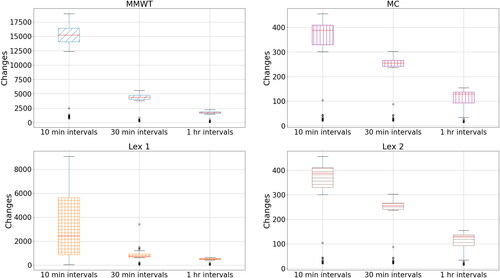
The results are shown in Figures 10 and 11. There are two important aspects to note. Firstly, the number of changes strongly reduces as the length of the time periods increases, across all approaches. Going from 10 min intervals (144 time periods) to 30 min intervals (48 time periods) gives reductions in changes ranging from 34% (MC and Lex 2) to 71% (MMWT). Going from 10 min to 1 h intervals (24 time periods) results in reductions ranging from 67% (MC and Lex 2) and 88% (MMWT). If there are fewer distinct time periods, there are fewer chances to change worker numbers.

However, this comes at the cost of increasing the max. workers. For example, the max. workers required for MC increased from a median of 464 to 555.5 (20% increase), when decreasing from 144 to 24 time periods. We also observe an 11% increase for Lex 2 (333 workers to 370), and a 3% decrease for MMWT and Lex 1. This is important—by considering longer time intervals, we reduce changes, but this requires more max. workers (though proportionally less) when considering MC and Lex 2 and sometimes even decreasing maximum workers required (for MMWT and Lex 1) because there is a more balanced spread of workers across the WAs due to the longer time intervals (i.e., a worker stays on for longer at the same WA).

6. Conclusion

Staffing in sequential sorting facilities is important, as upstream delays will propagate through the facility. We present a new model to solve this problem for several objectives that are important in practice. This is based on a network flow model but incorporates additional complexity, such as indirect streams and tethered WAs. We also account for time-dependency in sorting deadlines using a time-expanded network, at a very fine-grained timescale. This poses additional challenges as it increases the size of the network, and hence the model complexity.

We apply this model to data collected at a mail sorting facility over a time period of 3 months. The data includes daily mail volumes for different streams of mail (e.g., first class letters, second class letters), suggested staff workplans provided by the company, and details on sorting constraints for each stream. We compared the different approaches with each other, as well as against staff levels suggested by the UKMC. We also examined how the model performs under different scenarios. Namely, when mail volumes are increased, when the split between letters and parcels changes, and when the level of time discretisation is decreased.

When comparing all objectives, we naturally found that MMWT and Lex 1 were the best approaches regarding maximum workers, and MC and Lex 2 were the best regarding changes. However, Lex 2 consistently outperformed the UKMC on both considered objectives.

Increasing mail volumes resulted in more workers required, but the proportional increase in workers was less than that of the increase in mail. Changes also showed increases as the mail volumes increased.

The proportion of parcels vs letters also had an interesting effect on the results. Both max workers and changes increased as the proportion of parcels increased. This suggests that parcels are more labour-intensive to sort. Given the long term increasing trend in parcel volumes (and decreasing trend in letter volumes), this is important information for practitioners.

Finally, when changing the time granularity, reducing the number of time periods has differing effects, depending on the approach used. For Lex 2 and MC, there is a trade-off when reducing the time granularity, between reducing the number of changes, but increasing the max. workers. For Lex 1 and MMWT, the number of changes reduces, but there is also a slight reduction in the max. workers. This shows that there can be benefits to having a reduced time discretisation, but it is approach-dependent.

While the results are positive, there are some limitations to this work. We assume that the mail volumes are known before staff allocation. This is often unrealistic in practise. An avenue for future research would be to relax this assumption. For example, this could be formulated as a stochastic problem, with mail volumes treated as random variables, and including probabilistic constraints. Such an approach would need greater computational power to solve the model. Using or developing more sophisticated optimisation techniques to solve this is another area for future research.

We contribute to the staff rostering literature by showing the value of using network models to set short-term operational staff levels for sequential sorting facilities. We also highlight the importance of examining the priorities of differing objectives.

From a managerial perspective, our model allows decision makers to determine work plans balancing several objectives for their day to day operations. By analysing several scenarios and potential future trends, such as decreasing letter and increasing parcel volumes, decision makers can assess whether their current setup is appropriate to meet future challenges or whether adaptations are required.

Acknowledgements

We thank Marcos Charalambides and Tim Flack for their advice and support throughout this work. We would also like to acknowledge the High End Computing service at Lancaster University.

Disclosure statement

No potential conflict of interest was reported by the author(s).

Additional information

Funding

This paper is based on work completed while Hamish Thorburn was part of the EPSRC funded STOR-i centre for doctoral training (EP/S022252/1).

Appendix A

A.1 Computational performance

To examine the computational performance of the model, we report the optimality gap for each objective for each day. Given the effect that the level of time discretisation should have on these gaps, we plot them against time granularity, split by objective in Figure A1.

Note that the gaps for 10-min intervals should be representative of the gaps for all other experiments. We see that the gaps are very large for the Lex 1 objective, and (while smaller) are also still large for Lex 2. The gaps for MMWT and MC are much smaller, with MMWT having a median gap of 1.2%.

We see significant improvement in the gaps for MC, Lex 1, and Lex 2 as the level of time granularity is decreased (MMWT does not improve, primarily given how well it performs already).

A.2 UKMC algorithm for setting staff levels

The UKMC sets their workplans with an algorithm which:

1. Smooths the arrival of mail evenly between all time periods between its arrival time and the arrival time of the next delivery of mail.

2. Calculates the amount of mail going through each work area at each time period.

3. Divides the calculated mail traffic by the given throughput per processing unit (in this case, sorting machines) to obtain the number of machines.

4. Multiplies the number of machines by the number of workers required to work one machine to calculate the final number of workers in each time period in each work area.

A.3 Results with omissions

Figure A2 shows the total changes for the MC and Lex 2 objectives, along with those suggested by the UKMC. It is now clear that MC and Lex 2 show lower changes than the UKMC.

A.4 Constraining the secondary objective

We examine the effect of applying a bound on the secondary objective at various levels when minimising the first objective. This prevents the model from finding solutions that, while performing well on one objective, are extremely poor regarding the other. We set the constraints to be at most 50, 100, 500, and 1000% worse than the optimal value for the secondary objective. We then look at how much proportionally worse the primary objective becomes relative to its optimal value (which we found previously) when imposing this constraint.

As can be expected, tightening the bound on changes causes the minimum maximum number of workers to become worse (see Figure A3). This shows that while we can limit how many changes the model sets, this does come at a cost. The median increase in the max workers is 0.3% when the changes have to be within 500% of the minimum, $3\%$ if the changes have to be within 100%, and $8\%$ when the changes have to be within $50\%.$ We see similar results when changes is the primary objective. The main difference is that the bound on max workers needs to be much tighter to start affecting the number of changes (Figure A4). For 100, 500, and 1000% bounds, the median increase in the optimal number of changes is 0%. This shows that the minimum number of changes is less sensitive to these constraints on the max workers. We also included a bound of a 10% increase in the maximum workers, to see when the bound was tight enough to start affecting the workers. With the 10% increase, the median changes were 26% above their lowest possible values, showing that at this point, the bound is tight enough to start affecting the changes. While this can be useful in practice, an important question is which value for a bound is appropriate to avoid setting it arbitrarily. For this decision to be made, the whole optimisation model would need to be run first. In contrast, lexicographical optimisation ensures that (given the priorities of the objectives) we are achieving the lowest possible on one objective, and conditionally the lowest possible value on the second objective.

Figure A1. Optimality gap of the models vs. time granularity, split by objective.

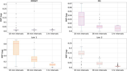
Figure A2. Boxplot of changes for the different objectives with MMWT and Lex 1 removed, for easier comparison.

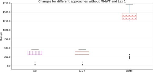
Figure A3. Increase in max workers by allowable increase in changes.

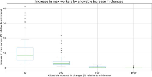
Figure A4. Increase in changes by allowable increase in max workers.

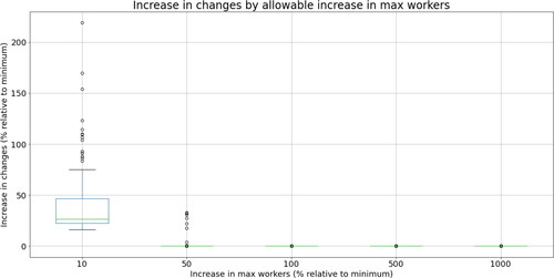
Figure 1. Diagram of a small example mail centre (Mech.: mechanically sorted; Man.: manually sorted).

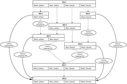
Figure 2. Base network of a small example of a mail centre.

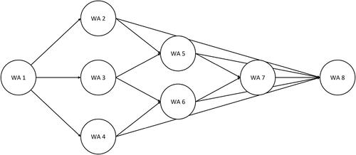
Figure 3. Time-expanded version of the base network from Figure 2 for eight time periods.

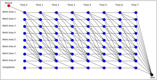
Figure 4. Boxplots of maximum workers for each day for the different approaches, as well as those recommended by the UKMC.

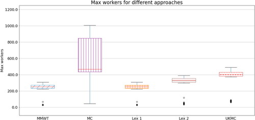
Figure 5. Boxplots of changes required for each day for the different approaches, as well as those recommended by the UKMC.

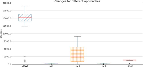
Figure 6. Max workers vs. mail volume increase for different approaches.

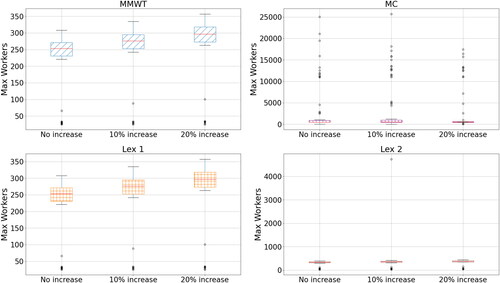
Figure 7. Changes vs. mail volume increase for the different approaches.

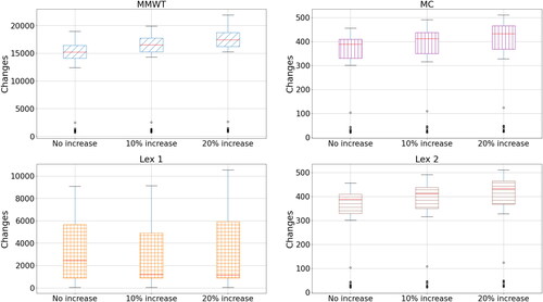
Figure 8. Max workers vs. proportion of letters. Eighty percent letters is the current baseline.

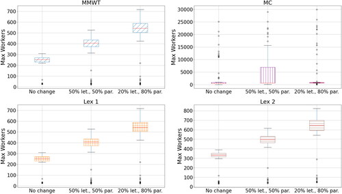
Figure 9. Changes vs. proportion of letters. Eighty percent letters is the current baseline.

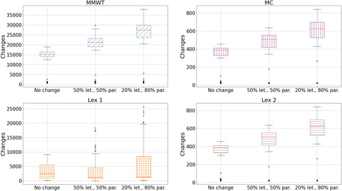
Figure 10. Max workers vs. different levels of time discretisation, split by approach.

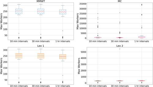
Figure 11. Changes vs. different levels of time discretisation, split by approach.

References

- Ahuja, R. K., Magnanti, T. L., & Orlin, J. B. (1994). Network flows: Theory, algorithms and applications (Vol. 50). Elsevier B.V.
- Andreatta, G., De Giovanni, L., & Monaci, M. (2014). A fast heuristic for airport ground-service equipment–and–staff allocation. Procedia-Social and Behavioral Sciences, 108, 26–36. https://doi.org/10.1016/j.sbspro.2013.12.817
- Bard, J. F., Binici, C., & deSilva, A. H. (2003). Staff scheduling at the United States Postal Service. Computers & Operations Research, 30(5), 745–771. https://doi.org/10.1016/S0305-0548(02)00048-5
- Bard, J. F., DeSilva, A., Feo, T. A., & Wert, S. D. (1993). Design of semi-automated mail processing facilities. IIE Transactions, 25(4), 88–101. https://doi.org/10.1080/07408179308964307
- Brucker, P., & Knust, S. (2012). Complex scheduling. Springer.
- Brunner, J. O., Bard, J. F., & Kolisch, R. (2009). Flexible shift scheduling of physicians. Health Care Management Science, 12(3), 285–305. https://doi.org/10.1007/s10729-008-9095-2
- De Bruecker, P., Van den Bergh, J., Beliën, J., & Demeulemeester, E. (2015). Workforce planning incorporating skills: State of the art. European Journal of Operational Research, 243(1), 1–16. https://doi.org/10.1016/j.ejor.2014.10.038
- Devesse, V. A. P. A., Akartunalı, K., Arantes, M. d S., & Toledo, C. F. M. (2022). Linear approximations to improve lower bounds of a physician scheduling problem in emergency rooms. Journal of the Operational Research Society, 74(3), 888–904. https://doi.org/10.1080/01605682.2022.2125841
- Ernst, A. T., Jiang, H., Krishnamoorthy, M., Owens, B., & Sier, D. (2004). An annotated bibliography of personnel scheduling and rostering. Annals of Operations Research, 127(1–4), 21–144. https://doi.org/10.1023/B:ANOR.0000019087.46656.e2
- Gurobi Optimization, LLC (2022). Gurobi optimizer reference manual. Retrieved from https://www.gurobi.co
- Jarrah, A. I. Z., Bard, J. F., & deSilva, A. H. (1994a). Equipment selection and machine scheduling in general mail facilities. Management Science, 40(8), 1049–1068. https://doi.org/10.1287/mnsc.40.8.1049
- Jarrah, A. I. Z., Bard, J. F., & deSilva, A. H. (1994b). Solving large-scale tour scheduling problems. Management Science, 40(9), 1124–1144. https://doi.org/10.1287/mnsc.40.9.1124
- Kabiru, S., Saidu, B. M., Abdul, A. Z., & Ali, U. A. (2017). An optimal assignment schedule of staff-subject allocation. Journal of Mathematical Finance, 7(4), 805–820. https://doi.org/10.4236/jmf.2017.74042
- Li, Y., Gao, X., Xu, Z., & Zhou, X. (2018). Network-based queuing model for simulating passenger throughput at an airport security checkpoint. Journal of Air Transport Management, 66, 13–24. https://doi.org/10.1016/j.jairtraman.2017.09.013
- Louly, M. (2013). A goal programming model for staff scheduling at a telecommunications center. Journal of Mathematical Modelling and Algorithms in Operations Research, 12(2), 167–178. https://doi.org/10.1007/s10852-012-9200-x
- Ni, H., & Abeledo, H. (2007). A branch-and-price approach for large-scale employee tour scheduling problems. Annals of Operations Research, 155(1), 167–176. https://doi.org/10.1007/s10479-007-0212-2
- OFCOM (2012). Communications market report 2012. Key Non Parliamentary Papers Ofcom (Office of Communications). Retrieved from https://www.ofcom.org.uk/_data/assets/pdf file/0013/20218/cmruk2012.pdf
- Paias, A., Mesquita, M., Moz, M., & Pato, M. (2021). A network flow-based algorithm for bus driver rerostering. OR Spectrum, 43(2), 543–576. https://doi.org/10.1007/s00291-021-00622-3
- Qi, X., & Bard, J. F. (2006). Generating labor requirements and rosters for mail handlers using simulation and optimization [Part special issue: Anniversary focused issue of Computers & Operations Research on tabu search]. Computers & Operations Research, 33(9), 2645–2666. https://doi.org/10.1016/j.cor.2005.02.022
- Restrepo, M. I., Lozano, L., & Medaglia, A. L. (2012). Constrained network-based column generation for the multi-activity shift scheduling problem. International Journal of Production Economics, 140(1), 466–472. https://doi.org/10.1016/j.ijpe.2012.06.030
- Skaugset, L. M., Farrell, S., Carney, M., Wolff, M., Santen, S. A., Perry, M., & Cico, S. J. (2016). Can you multitask? Evidence and limitations of task switching and multitasking in emergency medicine. Annals of Emergency Medicine, 68(2), 189–195. https://doi.org/10.1016/j.annemergmed.2015.10.003
- Tapkan, P., Kulluk, S., Özbakır, L., Bahar, F., & Gülmez, B. (2022). A constraint programming based column generation approach for crew scheduling: A case study for the Kayseri railway. Journal of the Operational Research Society, 74(9), 2028–2042. https://doi.org/10.1080/01605682.2022.2125843
- Tello, F., Jiménez-Martín, A., Mateos, A., & Lozano, P. (2019). A comparative analysis of simulated annealing and variable neighborhood search in the ATCo work-shift scheduling problem. Mathematics, 7(7), 636. https://doi.org/10.3390/math7070636
- Van den Bergh, J., Beliën, J., De Bruecker, P., Demeulemeester, E., & De Boeck, L. (2013). Personnel scheduling: A literature review. European Journal of Operational Research, 226(3), 367–385. https://doi.org/10.1016/j.ejor.2012.11.029
- Xie, L., & Suhl, L. (2015). Cyclic and non-cyclic crew rostering problems in public bus transit. OR Spectrum, 37(1), 99–136. https://doi.org/10.1007/s00291-014-0364-9
- Zhang, X., Chakravarthy, A., & Gu, Q. (2009). Equipment scheduling problem under disruptions in mail processing and distribution centres. Journal of the Operational Research Society, 60(5), 598–610. https://doi.org/10.1057/palgrave.jors.2602581
- Zhang, X., & Bard, J. F. (2005). Equipment scheduling at mail processing and distribution centers. IIE Transactions, 37(2), 175–187. https://doi.org/10.1080/07408170590885657