Assessment of the MODIS global evapotranspiration algorithm using eddy covariance measurements and hydrological modelling in the Rio Grande basin

Abstract

Remote sensing is considered the most effective tool for estimating evapotranspiration (ET) over large spatial scales. Global terrestrial ET estimates over vegetated land surfaces are now operationally produced at 1-km spatial resolution using data from the Moderate Resolution Imaging Spectroradiometer (MODIS) and the MOD16 algorithm. To evaluate the accuracy of this product, ground-based measurements of energy fluxes obtained from eddy covariance sites installed in tropical biomes and from a hydrological model (MGB-IPH) were used to validate MOD16 products at local and regional scales. We examined the accuracy of the MOD16 algorithm at two sites in the Rio Grande basin, Brazil, one characterized by a sugar-cane plantation (USE), the other covered by natural savannah vegetation (PDG) for the year 2001. Inter-comparison between 8-day average MOD16 ET estimates and flux tower measurements yielded correlations of 0.78 to 0.81, with root mean square errors (RMSE) of 0.78 and 0.46 mm d^-1, at PDG and USE, respectively. At the PDG site, the annual ET estimate derived by the MOD16 algorithm was 19% higher than the measured amount. For the average annual ET at the basin-wide scale (over an area of 145 000 km²), MOD16 estimates were 21% lower than those from the hydrological model MGB-IPH. Misclassification of land use and land cover was identified as the largest contributor to the error from the MOD16 algorithm. These estimates improve significantly when results are integrated into monthly or annual time intervals, suggesting that the algorithm has a potential for spatial and temporal monitoring of the ET process, continuously and systematically, through the use of remote sensing data.

Editor D. Koutsoyiannis; Associate editor T. Wagener

Citation Ruhoff, A.L., Paz, A.R., Aragao, L.E.O.C., Mu, Q., Malhi, Y., Collischonn, W., Rocha, H.R., and Running, S.W., 2013. Assessment of the MODIS global evapotranspiration algorithm using eddy covariance measurements and hydrological modelling in the Rio Grande basin. Hydrological Sciences Journal, 58 (8), 1658–1676.

Résumé

La télédétection est considérée comme l’outil le plus efficace pour estimer l’évapotranspiration (ET) sur de grandes échelles spatiales. Les estimations globales d’ET terrestre sur les surfaces végétalisées sont aujourd’hui produites de manière opérationnelle à une résolution kilométrique en utilisant les données du spectroradiomètre imageur à résolution moyenne (Moderate Resolution Imaging Spectroradiometer – MODIS) et l’algorithme MOD16. Pour évaluer la justesse de ce produit, nous avons utilisé des mesures au sol des flux d’énergie provenant à la fois de sites de covariance de la turbulence, installés dans des biomes tropicaux, et d’un modèle hydrologique (MGB-IPH), afin de valider les produits MOD16 aux échelles locale et régionale. Nous avons examiné l’exactitude de l’algorithme MOD16 sur deux sites au sein du bassin du Rio Grande, au Brésil, l’un correspondant à une plantation de canne à sucre (USE), l’autre étant couvert par une végétation de savane naturelle (PDG), pour l’année 2001. La comparaison entre les estimations MOD16 d’ET moyennées sur huit jours et les mesures de tours à flux a donné des corrélations de 0,78 à 0,81, avec des valeurs de la racine de l’erreur quadratique moyenne (RMSE) de 0,78 et 0,46 mm j^-1 respectivement sur les sites PDG et USE. Sur le site PDG, l’estimation de l’ET annuelle obtenue par l’algorithme MOD16 était de 19% supérieure à la quantité mesurée. Pour l’ET moyenne annuelle à l’échelle du bassin entier (d’une superficie de 145 000 km²), les estimations MOD16 étaient de 21% inférieures à celles du modèle hydrologique MGB-IPH. Les erreurs de classification de l’occupation des sols et du couvert végétal ont été identifiées comme la principale source d’erreur de l’algorithme MOD16. Ces estimations s’améliorent de manière significative lorsque les résultats sont intégrés sur des intervalles de temps mensuels ou annuels, ce qui suggère que l’algorithme a un potentiel pour le suivi spatial et temporel du processus d’ET, de manière continue et systématique, grâce à l’utilisation de données issues de la télédétection.

Key words:

• evapotranspiration
• hydrological modelling
• MGB-IPH
• MOD16
• MODIS

Mots clefs:

• évapotranspiration
• modélisation hydrologique
• MGB-IPH
• MOD16
• MODIS

1 INTRODUCTION

Estimations of evapotranspiration (ET) are essential for quantifying the responses of terrestrial ecosystem dynamics to climate (Churkina et al. 1999, Nemani et al. 2002). Evapotranspiration is strongly related to the energy transfer processes. Therefore, monitoring this process at both spatial and temporal scales is critical for improving our understanding of interactions between the land and atmosphere. This knowledge can be applied for: monitoring and predicting drought events (McVicar and Jupp 1998, Mu et al. 2013), managing water resources for agriculture (Gowda et al. 2009), and studying regional-scale hydrological processes (Kustas and Norman 1996, Rango and Shalaby 1998). Much effort has been devoted to improving spatial and temporal estimates of ET using remotely sensed data, at local scales (Bastiaanssen et al. 1998, Su 2002, Tasumi et al. 2005), regional scales (Venturini et al. 2008, Mallick et al. 2009, Bhattacharya et al. 2010, Jang et al. 2010), continental (Nishida et al. 2003, Cleugh et al. 2007) and global scales (Mu et al. 2007, Fisher et al. 2008, Mu et al. 2011, Vinukollu et al. 2011). However, accurate estimates of ET at large spatial scales are still challenging because of the high heterogeneity of the Earth’s surface characteristics which drive the ET process, including availability water, topography, vegetation cover, soil properties, as well as the variability of climate (Gash 1987, Friedl 1996, Janowiak et al. 1998). Moreover, ET estimates can be affected by inherent limitations of optical and thermal remotely sensed data, such as cloud cover, scale factors and the time intervals between successive image captures (Moran et al. 1997, Asner 2001, Couralt et al. 2005).

Developing an algorithm for estimating ET at the global scale is difficult due to the spatial complexity of the required atmospheric and surface inputs. For global purposes, the ET algorithm needs to be sufficiently complex to ensure a realistic representation of all physical processes, whilst being simple enough to allow the model to operate globally. The MOD16 algorithm (Mu et al. 2011) combines remotely sensed data on land use and land cover, albedo, leaf area index (LAI) and fraction of photosynthetically active radiation (fpar), with downward solar radiation (R_s), air temperature (T_a) and actual vapour pressure deficit (e_a) from re-analysis data to estimate global ET. The ET data derived from the MOD16 algorithm are available at 1-km spatial resolution over the 109.03 × 10⁶ km² global vegetated land areas at 8-day, monthly and annual intervals. The algorithm is based on the Penman-Monteith equation (Monteith 1965) to calculate transpiration from plant canopies, evaporation from intercepted precipitation by the canopy and soil evaporation. Stomatal conductance (c_s) and canopy conductance (c_c) are controlled by vapour pressure deficit (VPD) and minimum daily air temperature (T_min) (Oren et al. 1999, Heinsch et al. 2003, Running et al. 2004).

To contribute to further improvements and development of the MODIS global ET product, our general aim in this paper is to critically evaluate the performance of the MOD16 algorithm over an agricultural area covered by sugar-cane plantation and natural savannah vegetation in Brazil during the year 2001. Specifically, we aim to:

• – analyse the MOD16 algorithm estimates at a range of time scales (8-day, monthly and annual) and spatial scales (site and basin-wide scales);

• – compare the MOD16 algorithm estimates with eddy covariance data recorded at two flux tower sites installed in areas of natural savannah vegetation (PDG site) (Rocha et al. 2002) and sugar-cane cropland (USE site) (Cabral et al. 2003); and

• – compare the MOD16 algorithm estimates with ET estimates from the hydrological model MGB-IPH (Collischonn et al. 2007a).

2 STUDY AREA

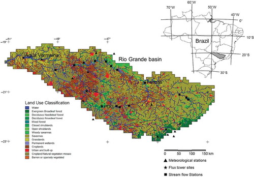
The study was carried out in the Rio Grande basin, Brazil. This is an area of natural savannah, lying between latitudes 19°15′ and 23°00′ S and longitudes 43°30′and 51°00′ W (Fig. 1). The basin is located in southeastern Brazil and includes two Brazilian States, São Paulo and Minas Gerais. The Rio Grande basin drains an area of about 145 000 km². Its main river is the Rio Grande, which is one of the main tributaries of the Paraná River. Most of the basin is covered by savannah vegetation, locally called cerrado. This natural vegetation was extensively replaced during the last century (1900–2000) by intensive production of sugar-cane and soy, and by pasture (Loarie et al. 2011). Variations in vegetation physiognomy are characterized by changes in elevation, soil properties and climate, followed by changes in vegetation density. The floristic composition of this natural vegetation can be divided into five classes: (a) campos limpos, characterized by the dominance of grasses with an average height of 0.5 m; (b) campos sujos, which is grasslands with sparse occurrence of shrubs of 2 m height on average; (c) campos cerrados, which is physionomically dominated by grasses and shrubs, but with the occurrence of sparse trees reaching a maximum height of 5 m; (d) cerrado, which consists of dense vegetation dominated by shrubs and trees of 5–10 m height; and (e) cerradão, characterized by semi-deciduous seasonal forest, with trees mostly over 10 m height and poorly developed grass cover (Eiten 1972, Batalha 1997, Furley 1999).

Fig. 1 Land-use and land-cover classification based on MOD12Q1 for 2001 at the Rio Grande basin (Brazil). The 14 meteorological stations, 15 streamflow stations (including Agua Vermelha and Furnas) and two flux towers (PDG and USE) used in this study are displayed.

The regional climate is classified as humid subtropical (Koppen classification Cwa or Cfa). The average monthly temperatures range from 17.6 to 23.5°C. The average annual precipitation is about 1500 mm, concentrated mostly in the austral summer (November–April) and the annual ET is approximately 900 mm (Rocha et al. 2002). The natural savannah ET has a strong seasonality, ranging from 1 mm d^-1 in the dry season to 6 mm d^-1 in the wet season (Rocha et al. 2002). In agricultural areas, ET varies according to the type of the cropland and its cultivation cycle, with significant variations due to vegetation structure that may range from bare soil areas to fully developed canopy cover.

3 MATERIALS AND METHODS

3.1 MOD16 algorithm

3.1.1 Algorithm description

The MODIS global ET algorithm is a part of NASA’s Earth observing system for estimating ET from Earth’s land surface using MODIS remote sensing data for hydrological and ecological applications. The MOD16 (Mu et al. 2011) (equation (1)) product is based on the beta version of the algorithm (Mu et al. 2007) developed from Cleugh et al. (2007), using a Penman-Monteith approach (Monteith 1965):

(1)

where ET is the daily evapotranspiration (mm d^-1); (Pa K^-1) is the gradient of saturated vapour pressure to air temperature; R_n (J d^-1) is the net radiation; G (J d^-1) is the soil heat flux; ρ_a is the air density (kg m^-3); C_p (J kg^-1 K^-1) is the specific heat of air at constant pressure; e_s and e_a (Pa) are the saturated vapour pressure and actual vapour pressure, respectively; γ (0.066 kPa K^-1) is the psychometric constant; whilst r_s and r_a (s m^-1) are the surface and aerodynamic resistance, respectively.

Improvements of the MOD16 algorithm (Mu et al. 2011) in relation to its previous version (Mu et al. 2007) include:

1. separation of the canopy into wet and dry surface, which provides water loss estimates of canopy evaporation from the wet canopy surface and the canopy transpiration from the dry surface;

2. consideration of wet surface and soil moisture, in which the ground surface evaporation includes potential evaporation from the wet surface and evaporation from the soil;

3. inclusion of daytime and night-time ET estimates;

4. the amount of soil heat flux is estimated and now only occurs to the radiation partitioned to the ground surface; and

5. improvement of methods for estimating c_s and c_c, aerodynamic resistance and vegetation cover fraction.

Full details of the MOD16 algorithm and its improvements are given by Mu et al. (2011).

3.1.2 Remote sensing inputs

Remote sensing inputs derived from three MODIS products, with a spatial resolution of 500–1000 m are used as land surface inputs. These products include:

1. MOD12Q1 Collection 5 (land-use and land-cover classification) (Friedl et al. 2002);

2. MOD15A2 Collection 5 (LAI and fpar) (Myneni et al. 2002); and

3. MCD43B2/B3 Collection 5 (albedo) (Lucht et al. 2000, Schaaf et al. 2002, Jin et al. 2003, Salomon et al. 2006).

MOD15A2 and MCD43B3 gap-filling data entail two steps based on the corresponding quality control (QC) product MCD43B2 (Zhao et al. 2005):

1. if the 8-day pixel was missing or unreliable it was replaced by the closest reliable 8-day pixel; and

2. other unreliable pixels were replaced by simple linear interpolation of the nearest reliable pixels prior to and after the temporal missing pixels.

3.1.3 GMAO meteorological inputs

Global Modelling and Assimilation Office (GMAO) re-analysis data with a spatial resolution of 1.0° × 1.25° (GMAO 2004), provided at every one hour were used as meteorological inputs. We processed the hourly data to get daily total downward radiation (R_s, MJ d^-1), daily average air temperature (T_avg, °C), daytime and night-time air temperatures (T_{day_avg}, T_{night_avg}, °C), daily minimum air temperature (T_min, °C) and vapour pressure (e_s, e_a, kPa). To reconcile the meteorological inputs, data were interpolated from coarse spatial resolution to 1 km to fit the MODIS pixels, to remove abrupt changes from one side of a GMAO pixel to another and improve the accuracy of these pixels, using a fourth power cosine function proposed by Zhao et al. (2005).

3.2 MGB-IPH hydrological model

3.2.1 Hydrological model description

The MGB-IPH is a distributed hydrological model developed for large basins with drainage area over 10 000 km² (Collischonn et al. 2007a). This model calculates the complete water balance at daily or monthly time intervals. We run the model using a regular grid with a spatial resolution of 10 km. The grid cells were connected by channels representing the drainage network (Paz and Collischonn 2007). Each grid cell was divided into classes that combine soil type and vegetation, which are called Hydrological Response Units (HRU) (Kouwen et al. 1993, Beven 2001) to account for the fractional contributions from different physical characteristics within each grid cell. In the MGB-IPH model, evaporation of water (from soil, open water and intercepted water) and the transpiration (from plants) were calculated separately based on the Penman-Monteith equation (equation (1)), using the approach of Wigmosta et al. (1994). It is assumed that actual evaporation of water intercepted by the canopy (EI, mm d^-1) is prioritized over soil evaporation and plant transpiration. Evaporation of soil water occurs subsequently. If there still is a demand for evaporation, then water is evaporated from a second soil layer. The maximum depth of canopy intercepted water (EI_max) was determined for each HRU as a function of LAI (Ubarana 1996) (equation (2)). The LAI (m² m^-2) value is a function of land use and land cover in each HRU:

(2)

After estimating evaporation from intercepted water and soil evaporation, the remaining evaporative demand fraction (f_DE) (equation (3)) was met by plant transpiration for each vegetation type, which was used as a correction factor to calculate the plant transpiration (equation (4)):

(3)

(4)

where EIP (mm d^-1) is the potential evaporation of intercepted water, considering that r_s = 0 (for EI > EIP, otherwise EI = EIP); λ (J kg^-1) is the latent heat of evaporation; and ρ_w (kg m^-3) is the water density. In this model, aerodynamic resistance (r_a) depends only on the canopy height (m) and wind speed (U, m s^-1), whilst surface resistance (r_s) is a characteristic of each vegetation type at ranges according to the restriction of soil moisture (W, mm). It is assumed that soil conditions do not restrict ET if soil moisture exceeds 50% of soil water content at field capacity (W_M, mm) (Shuttleworth 1993). In this case, surface resistance is regarded as a minimum value typical of vegetation unaffected by soil moisture conditions. If soil moisture lies between soil at wilting point (W_WP, mm) and soil at the plant stress point (W_L, mm), surface resistance increases and ET reduces (equation (5)) (Wigmosta et al. 1994). If soil moisture is lower than the wilting point, the restriction is at its maximum and ET is zero. For simplification, W_PM was set at 10%, while W_L was set at 50% of soil water content at field capacity:

(5)

where r_sm (s m^-1) is surface resistance for a given soil moisture that does not restrict ET. Full details of the soil water balance in the MGB-IPH are given by Collischonn et al. (2007a). This model was chosen for use in this research because it was developed specifically for large South American basins, was previously applied and tested in several basins (Collischonn et al. 2005, 2006, Getirana et al. 2010, Nóbrega et al. 2011, Paiva et al. 2011), and, moreover, because this model had already been calibrated and validated for the study area for flow forecasting purposes with an error of less than 7% (Collischonn et al. 2007b, Tucci et al. 2008, Bravo et al. 2009, Nóbrega et al. 2011).

Table 1 Description of evapotranspiration parameters used for the MGB-IPH hydrological model calibration

Parameter	HRU	Jan.	Feb.	Mar.	Apr.	May	Jun.	Jul.	Aug.	Sep.	Oct.	Nov.	Dec.
Albedo	1	0.13	0.13	0.14	0.15	0.16	0.16	0.17	0.17	0.16	0.15	0.14	0.13
	2	0.13	0.13	0.14	0.15	0.16	0.16	0.17	0.17	0.16	0.15	0.14	0.13
	3	0.15	0.15	0.15	0.15	0.16	0.16	0.18	0.18	0.17	0.16	0.15	0.15
	4	0.13	0.13	0.13	0.13	0.13	0.13	0.13	0.13	0.13	0.13	0.13	0.13
	5	0.13	0.13	0.14	0.15	0.16	0.16	0.17	0.17	0.16	0.15	0.14	0.13
	6	0.1	0.1	0.1	0.1	0.1	0.1	0.1	0.1	0.1	0.1	0.1	0.1
LAI (m^2 m^-2)	1	4	4	4	3	2	1	1	1	1	2	3	4
	2	6	6	4	3	2	1	1	1	1	2	3	4
	3	2	2	2	2	2	1	1	1	2	2	2	2
	4	6	6	5	4	3	3	3	3	3	4	4	5
	5	4	4	4	3	2	1	1	1	1	2	3	4
	6	0	0	0	0	0	0	0	0	0	0	0	0
Canopy height (m)	1	1	1	1	1	1	1	1	1	1	1	1	1
	2	1	1	1	1	1	1	1	1	1	1	1	1
	3	0.5	0.5	0.5	0.5	0.5	0.5	0.5	0.5	0.5	0.5	0.5	0.5
	4	9	9	9	9	9	9	9	9	9	9	9	9
	5	0.5	0.5	0.5	0.5	0.5	0.5	0.5	0.5	0.5	0.5	0.5	0.5
	6	0.05	0.05	0.05	0.05	0.05	0.05	0.05	0.05	0.05	0.05	0.05	0.05
Surface resistance (s m^-1)	1	60	60	60	70	70	80	80	80	90	80	70	60
	2	60	60	60	70	70	80	80	80	90	80	70	60
	3	60	60	60	60	60	60	60	60	60	60	60	60
	4	90	90	90	90	90	90	90	90	90	90	90	90
	5	60	60	60	70	70	80	80	80	90	80	70	60
	6	0	0	0	0	0	0	0	0	0	0	0	0

3.2.2 Hydrological model calibration and validation

The calibration and validation procedures and results are fully presented in Collischonn et al. (2007b) and partially described in Tucci et al. (2008), Bravo et al. (2009) and Nóbrega et al. (2011). Therefore, just a brief summary is presented here. The hydrological model calibration and validation were performed using data from raingauges, streamflow and meteorological stations (Fig. 1). Data from 273 raingauges distributed over the basin and 15 streamflow stations were obtained from the Brazilian Water Agency, Agência Nacional de Águas (ANA 2010) and from the Integrated System for Water Resource Management of the State of São Paulo, Coordenadoria de Recursos Hídricos do Estado de São Paulo (CRH 2010). Meteorological data were obtained from data collection 14 platforms provided by the National Institute for Space Research in Brazil, Instituto Nacional de Pesquisas Espaciais (INPE 2010). Soil type information from the project RADAM Brasil (Ministério das Minas e Energia 1982), as well as land-use data derived from classification of Landsat 7 ETM+ images (Global Land Cover Facility 2010), were used to characterize each HRU. Landsat 7 ETM+ images were classified into four distinct groups: (a) open water, (b) forest (including reforestation), (c) cropland, and (d) grassland (including bare soil). Soil types were regrouped into three basic classes according to water storage capacity: high, medium or low. After merging all the information on soil type and land use, six HRUs were defined for the Rio Grande basin:

1. grassland and cropland areas with soils of medium storage capacity,

2. cropland areas with soils of high storage capacity,

3. soils with low storage capacity,

4. forest areas with soils of medium storage capacity,

5. grassland and bare soil with soils of high storage capacity, and

6. open water.

The model was run at a daily time interval. The period from 1970 to 1980 was used for calibrating the model and the period from 1981 to 2001 was used for validating the model. The adjusted parameter values, such as albedo, LAI, canopy height and surface resistance were derived from the literature (Table 1).

3.3 Eddy covariance flux tower sites

To validate the MOD16 algorithm and MGB-IPH model results, ground-based measurements obtained from eddy covariance flux towers located in areas of natural savannah (PDG site) and sugar-cane cropland (USE site) were used. Net radiation (R_n), latent heat (LE), sensible heat (H) fluxes and ancillary meteorological data were measured at a height of 21 m (at PDG) and 7 m (at USE) and recorded every half-hour. The ground-based data used in this paper were collected from October 2000 to December 2002 at the PDG site and from January 2001 to December 2002 at the USE site. There were missing eddy covariance data measurements during January 2001 and from August to December 2001 at the USE site, and also during a few days of January and September 2001 at the PDG site. Rocha et al. (2002), Juárez (2004) and Cabral et al. (2003) report full details of the equipment and measurement procedures used at the USE and PDG sites.

3.4 Data analysis

The measured eddy covariance data were averaged to daily, 8-day, monthly and annual time steps for comparison with both the MOD16 algorithm and MGB-IPH estimates. Daily and 8-day averages were not gap-filled and any given daily average with fewer than 75% of half-hourly data available was excluded from the analysis. Monthly and annual ET were calculated based on the daily data. Missing daily ET observations were interpolated based on the monthly average. The accuracy assessment of the MOD16 algorithm and the MGB-IPH model were performed by comparing predicted values from both models against ground-based observations at the two contrasting land cover sites. Moreover, the spatial accuracy at the basin-wide scale and the water balance closure were evaluated by comparing MOD16 predicted values against MGB-IPH. The performance of the models was quantified based on the root mean square error (RMSE), mean absolute error (MAE), Nash-Sutcliffe coefficient (NS), and coefficients of correlation (r) and determination (r²). To explain the variance in the predicted ET, we calculated the coefficient of determination between the MOD16 algorithm and the input data, such as MODIS remotely-sensed data and GMAO meteorological data.

4 RESULTS

4.1 Calibration and validation of the MGB-IPH hydrological model

To calibrate and validate the MGB-IPH model, observed values at 15 streamflow stations were compared with the predicted data. During the calibration period (1970–1980), NS coefficients ranged between 0.76 and 0.93, whilst errors in volume were lower than 0.05%. During the validation period (1981–2001), NS coefficients ranged between 0.82 and 0.95, with errors in volume of between –3.8% and 6.7%. Figure 2 presents the comparison between observed and calculated hydrographs at two ground stations, Furnas (drainage area 52 000 km²) and Agua Vermelha (drainage area 139 000 km²) on the Rio Grande River. The results demonstrated that the model can reproduce the natural river flow regime during both calibration and validation periods.

Fig. 2 Comparison between observed and calculated hydrographs during both calibration and validation periods at two major control points (Furnas and Agua Vermelha) along the Rio Grande.

4.2 Validation of estimated ET at flux tower level

4.2.1 Seasonal variability in 8-day average ET

To compare eddy covariance measurements and model predictions, MOD16 ET estimates were averaged over a 3 km × 3 km window surrounding the PDG and USE flux towers. The MODIS land-cover classification indicates that PDG is located in an evergreen broadleaf forest, while USE is in sugar-cane cropland. However, according to our classification results and field knowledge, the actual land cover at the PDG site is savannah or woodland savannah. For the MGB-IPH model, estimates at the PDG site were compared with HRU 4 (forest areas within soils of medium storage capacity) and USE site estimates were compared to HRU 2 (cropland within soils of high storage capacity), lying in the same HRUs as the flux towers.

At PDG, the eddy covariance 8-day average ET was 2.5 ± 1.2 mm d^-1, whilst the ET estimated by the MOD16 algorithm and MGB-IPH model were 3.2 ± 0.9 and 2.6 ± 1.0 mm d^-1, respectively. The 8-day MOD16 ET estimations yielded a correlation of 0.78 (p < 0.05, n = 39) with a RMSE of 0.78 mm d^-1 and a MAE of 0.54 mm d^-1 when compared against eddy covariance measurements. The 8-day MGB-IPH ET estimations yielded a correlation of 0.85 (p < 0.05, n = 39) with a RMSE of 0.60 mm d^-1 and a MAE of –0.09 mm d^-1 when similarly compared against eddy covariance measurements. These results indicate that the MOD16 algorithm overestimates (in both wet and dry seasons), while MGB-IPH slightly underestimates (mainly in the wet season) the measured ET at the PDG site.

At USE, the eddy covariance 8-day average ET was 2.5 ± 1.1 mm d^-1, whilst the ET estimated by the MOD16 algorithm and MGB-IPH model were 2.5 ± 1.4 and 2.8 ± 1.2 mm d^-1, respectively. At this site, 8-day MOD16 ET estimations yielded a correlation of 0.82 (p < 0.05, n = 20), with a RMSE of 0.46 mm d^-1 and a MAE of 0.02 mm d^-1 when compared against eddy covariance measurements. This result indicates almost no long-term over- or underestimation by the MOD16 algorithm in sugar-cane cropland. At this site, 8-day MGB-IPH ET estimations yielded a correlation of 0.96 (p < 0.05, n = 20), with a RMSE of 0.25 mm d^-1 and a MAE of –0.12 mm d^-1 when compared against eddy covariance measurements, indicating an underestimation of the modelled ET. However, both comparisons (MOD16 algorithm and MGB-IPH model against ground-based measurements) at USE should be analysed carefully, not only because of the limited number of 8-day average values, but also because of the sampling period from February (wet season ending) to August (dry season ending), which excludes important periods such as the transition between wet and dry seasons and the beginning of the wet season.

Seasonal variations in MOD16 ET estimates at the PDG (Fig. 3(a)) and USE (Fig. 3(b)) sites show almost the same temporal patterns as the ground-measured ET. At PDG, the MOD16 algorithm overestimates ET in both dry and wet seasons when compared against eddy covariance measurements. During the wet season, the overestimation ranges between 0.5 and 1.0 mm d^-1, while at the beginning of the dry season overestimation is reduced to less than 0.5 mm d^-1. During the beginning of the wet season, which normally starts in September, the MOD16 algorithm anticipates the increase in ET by almost two months. On average, actual ET starts to increase in early September, but the rise of MOD16 ET estimates begins in the middle of June, coincident with the winter solstice and the increase in R_s. For the MGB-IPH model, the wet season begins in September and the increase of the estimated ET is properly represented, following precipitation increase and soil moisture recovery.

Fig. 3 Seasonal variation of the 8-day average ET estimated from the MGB-IPH hydrological model and the MOD16 algorithm compared to eddy covariance (EC) measurements at (a) the PDG site and (b) the USE site. The climatological dry season is shaded and the top vertical bars represent the cumulative water deficit (computed by ET less precipitation plus the cumulative water deficit from the previous month). Error bars represent the standard error for each data point.

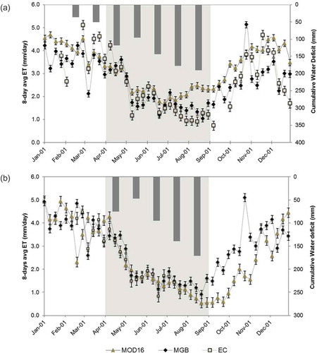
Because of missing data, the performance of the MOD16 algorithm and MGB-IPH model at the beginning of the wet season was not assessed at the USE site. However, we found that MOD16 and MGB-IPH ET estimates are significantly different in the period after the dry season, with differences higher than 1.5 mm d^-1 during August and November. The increase in the MOD16 estimates after the end of the dry season began in late September, according to the seasonal variations in LAI, fpar and VPD. Therefore, to understand what controls ET estimation in the MOD16 algorithm, and to test the hypothesis that ET is mainly driven by R_s at the PDG site and by LAI, fpar and VPD at the USE site, we calculated the correlation between predicted MOD16 ET and the algorithm input data to explain the variance in the predicted data (see Section 5.1, Controlling variance of ET in the MOD16 algorithm).

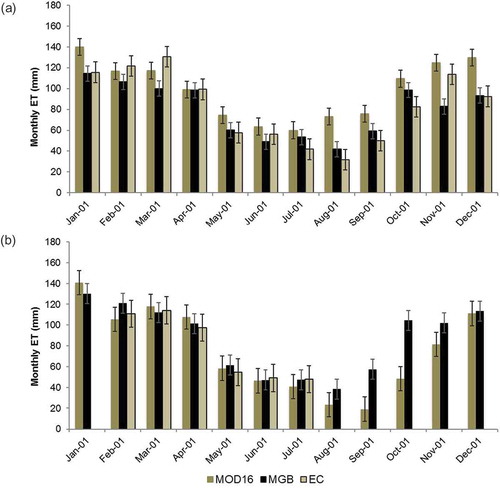
Fig. 4 Monthly ET estimated from the MGB-IPH hydrological model and the MOD16 algorithm compared to eddy covariance (EC) measurements at (a) the PDG site and (b) the USE site. Error bars represent the standard error for each data point.

4.2.2 Monthly and annual ET

Figure 4 shows monthly ET estimated from the MGB-IPH model and from the MOD16 algorithm compared to eddy covariance measurements. At the PDG site, MGB-IPH monthly estimates yielded a correlation of 0.91 (p < 0.05, n = 12) when compared against eddy covariance measurements. Monthly differences between estimated and measured values ranged from 1 to 30 mm, with a RMSE of 11 mm (15%) and MAE of –3 mm. The annual ET estimated by the MGB-IPH was 957 mm and the measured ET was 993 mm, a difference of less than 4%. Using the MOD16 algorithm, predicted monthly values generated a correlation of 0.89 (p > 0.05, n = 12), when compared against eddy covariance measurements, with a RMSE of 19 mm (32%) and MAE of 15 mm. Monthly differences between predicted and measured data ranged from 0 to 40 mm. The annual MOD16 ET estimate at PDG was 1183 mm, 19% higher than the measured ET and 23% higher than the MGB-IPH estimates.

At the USE site, the coefficient of correlation between the MGB-IPH monthly estimates and the eddy covariance measurements was 0.98 (p > 0.05, n = 6), with a RMSE of 4.5 mm (5%) and a MAE of 2 mm. Moreover, we found a coefficient of correlation of 0.97 (p > 0.05, n = 6), with RMSE of 5.5 mm (6%) and MAE of less than 0.5 mm between MOD16 algorithm and eddy covariance measurements. Annual ET estimated by the MGB-IPH model was 1038 mm, while ET estimated from the MOD16 algorithm was 893 mm, about 14%. We did not calculate measured annual ET at the USE site because of the missing data.

4.3 Validation of estimated ET at the basin scale

For the basin-wide analysis, we compared both the MOD16 algorithm and MGB-IPH with average ET values from the literature for the different land cover types (Table 2). This evaluation showed that estimates from MOD16 algorithm are within the range of values presented in the literature, although it has a tendency to underestimate the average ET at the basin scale for almost all land uses and land cover types. It is important to note that areas classified as forests (evergreen and deciduous broadleaf forest) in MOD12Q1 have average ET values equivalent to tropical rainforests, which explains the overestimation of ET in misclassified savannahs and woodland savannah areas.

Table 2 Daily average ET for the Rio Grande basin estimated by MOD16 algorithm during 2001 compared to average values of ET accepted in the scientific literature for different land-use and land-cover classifications

	Area	MOD16	Measured ET	Reference
	(%)	(mm d^-1)	(mm d^-1)
Savannah	37.27	1.95	2.3	Rocha et al. (2002)
Cropland and natural mixed vegetation	25.40	2.15	n.a.	n.a.
Cropland	17.84	2.09	2.5	Cabral et al. (2003)
			2.9	Watanabe et al. (2004)
Grassland and pasture	6.73	1.63	1.2∼2.0	Ferretti et al. (2003)
			2.6	Eugster and Cattin (2007)
Woodland savannah	5.34	2.19	2.8	Vourlitis et al. (2002)
Evergreen broadleaf forest	3.48	3.07	3.1	Hutyra et al. (2007)
			3.5	Rocha et al. (2004)
			3.9	Shuttleworth (1989)
Others	3.90	1.69	n.a.	n.a.
Total	100	2.00	n.a.	n.a.

Note: n.a.: data not available.

The comparison between the MOD16 and MGB-IPH 8-day averages for the entire Rio Grande basin showed a higher coefficient of correlation during the dry season (r = 0.92, p < 0.05) than during the wet season (r = 0.63, p < 0.05). The dry season also had a lower RMSE (0.26 mm d^-1) than the wet season (0.87 mm d^-1). The most significant differences between the two models occur in the wet season, when the MOD16 algorithm underestimates ET in comparison to the MGB-IPH model, for both 8-day average and for monthly values. At the annual time scale, the predicted ET based on the MOD16 algorithm was 773 mm year^-1, while the predicted ET based on MGB-IPH was 933 mm year^-1, with a difference of 21% between the two models.

To compare the spatial pattern predicted by the two models, we resampled MOD16 ET from the 1-km pixel size to a 10-km pixel size using an average filter, in order to match the spatial resolution of the MGB-IPH model. A pixel-by-pixel coefficient of determination (r²) and a standardized RMSE (RMSE_std) were calculated for each climatological season data set. To calculate the standardized error, we divided the RMSE of each pixel by the maximum RMSE (RMSE_max).

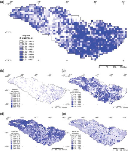
For the 8-day averages, there was a significant spatial coefficient of determination between the two models, with an average of 0.61 (the lowest pixel-by-pixel r² found was 0.11 and the highest was 0.87; n = 46), showing that the predicted ET values from the two models have a similar spatial pattern (Fig. 5(a)). We obtained an average r² of 0.40 (the lowest r² found was 0.02 and the highest was 0.88; n = 20) during the dry season (Fig. 5(b)) and during the wet season (Fig. 5(c)) a r² of 0.12 (lowest r² 0.01 and highest 0.58; n = 26). In the dry season, RMSE_max obtained from the two models was 1.7 mm d^-1 and the average RMSE_std for the entire basin was 0.30 ± 0.11 (Fig. 5(d)). In the wet season, RMSE_max was 2.6 mm d^-1 and the average RMSE_std was 0.55 ± 0.15 (Fig. 5(e)).

Fig. 5 Coefficient of determination (r²) during (a) both the wet and dry seasons, (b) the wet season, and (c) the dry season; and the seasonal standardized RMSE (RMSE_std) for (d) the wet season and (e) the dry season. To compute r² and RMSE_std we used 8-day average ET estimated from the MOD16 algorithm and MGB-IPH hydrological model.

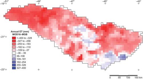
The pixel-by-pixel difference between annual ET estimated by the MOD16 algorithm and by the MGB-IPH model (Fig. 6) ranged from –475 to 432 mm, with an average of –200 mm, confirming that the MOD16 algorithm tends to underestimate ET in comparison to the MGB-IPH model. Areas where ET was underestimated are classified as cropland, savannahs, grasslands and mixed areas, while areas where ET was overestimated are mainly classified as evergreen broadleaf forest. Since the land use and land cover within the basin is predominantly savannah and agriculture, the underestimation of ET may be associated with underestimation and low seasonal amplitude of LAI, and low stomatal (c_s) and canopy (c_c) conductance.

Fig. 6 Annual ET differences between the MOD16 algorithm and MGB-IPH hydrological model predictions.

5 DISCUSSION

5.1 Controlling variance of ET in the MOD16 algorithm

The biome properties look-up table controls water and temperature stress related to land-use and land-cover classification. Because these parameters change plant transpiration significantly, the accuracy of the MOD16 algorithm is likely to be intrinsically driven by the quality of land-use and land-cover classification from MOD12Q1. During the year 2001, the PDG site was misclassified in MOD12Q1 as evergreen broadleaf forest, while the correct classification should have been savannah or even woodland savannah. The USE site was correctly classified as cropland. To explain the variance in the predicted ET, we calculated the coefficient of determination (r²) between MOD16 ET and the algorithm input data (Table 3), such as MODIS remotely-sensed data (Fig. 7) and GMAO meteorological data (Fig. 8).

Table 3 Explained variance between MOD16 ET estimations and input variables to the MOD16 algorithm at the PDG (savannah) and USE (sugar-cane) flux tower sites. (n = 46)

	PDG site	USE site
LAI	0.57	0.83
fpar	0.17	0.85
Albedo	0.36	0.32
Rs	0.69	0.13
ea	0.61	0.74
Tmin	0.52	0.22
Tavg	0.41	0.08
Tday_avg	0.45	0.09

Fig. 7 Scatter plots between 8-day average ET estimated from the MOD16 algorithm and MODIS remotely sensed input data at the PDG (left) and USE (right) sites. Error bars represent the standard error for each data point.

Fig. 8 Scatter plots between 8-day average ET estimated from the MOD16 algorithm and GMAO meteorological input data at the PDG (left) and USE (right) sites. Error bars represent the standard error for each data point.

At the PDG site, R_s explained over 57% of the variance of predicted MOD16 ET, since this site is classified as evergreen broadleaf forest having high stomatal (c_s) and canopy (c_c) conductance and low surface resistance (r_s), so giving high transpiration rates. Almost all radiation is converted into ET, which explains the increase in ET about two months before the beginning of the wet season and coincident with the winter solstice. Predicted LAI based on MODIS data (MOD15A2) was overestimated at this site, ranging between 5.0 and 6.7 m² m^-2, values that are appropriate for tropical rainforest (Wasseige et al. 2003, Aragão et al. 2005a, 2005b, Myneni et al. 2007). In areas of savannahs and woodland savannahs, LAI ranges from 1.8 to 2.9 m² m^-2 (Bitencourt et al. 2007) and in transitional areas between savannahs and tropical rainforests, LAI ranges from 2.5 to 5.5 m² m^-2 (Pinto et al. 2010), in dry and wet seasons, respectively. Therefore, overestimations of LAI associated with the misclassification in MOD12Q1 probably explain why ET is overestimated in this site.

At the USE site, the variance in ET is mainly controlled by fpar, LAI and e_a, in which each variable explains 85%, 83% and 74%, respectively. These variables are connected to vegetation phenology and water stress. Seasonal variations in ET follow the seasonal variations in LAI, fpar and actual vapour pressure, explaining the delay of about one month in the increase in ET after the beginning of the wet season. The differences of 1.5 mm d^-1 between MOD16 and MGB-IPH estimates after the end of the dry season may also be explained by the underestimation of LAI in MOD15A2; it ranges from 0.4 to 2.0 m² m^-2, while observed LAI of sugar-cane cropland in the tropics ranges from 0.9 to 5.0 m² m^-2 (Roberson et al. 1999).

5.2 MOD16 algorithm parameter fitting based on land use and land cover

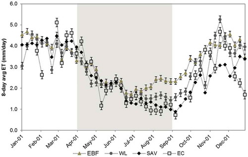
To understand the influence of land-use and land-cover classification on the MOD16 ET algorithm, LAI, fpar, albedo and the biome properties look-up table parameters at PDG site were adjusted to match a new land-use and land-cover classification (MOD12Q1) equivalent to savannah and woodland savannah. New values of LAI, fpar and albedo were extracted over a 7 km × 7 km window surrounding the PDG site. Of the 49 pixels, 32 were classified as evergreen broadleaf forest, five as savannah, five as woodland savannah, four as bare soil or sparsely vegetated, two as open shrub land and one as open water. After extracting these values, LAI, fpar and albedo were averaged for the woodland savannah and savannah classification. The values changed significantly: for woodland savannah, LAI values ranged from 1.0 to 3.2 m² m^-2, while for savannah, variation was between 0.5 and 2.5 m² m^-2, in dry and wet seasons, respectively (original LAI for evergreen broadleaf forest classification ranged from 5.0 to 6.7 m² m^-2). After running the MOD16 ET algorithm with parameters adjusted to woodland savannah and savannah, the accuracy of the 8-day average ET was satisfactorily better than the MOD16 ET with parameters misclassified as evergreen broadleaf forest (Table 4). Compared to the eddy covariance 8-day average ET, we found better correlations and lower RMSE and MAE for woodland savannah and savannah classifications in relation to evergreen broadleaf forest classification. In the same way, the annual ET for woodland savannah was 1048 mm, 6% higher than eddy covariance measurements, while for the savannah classification annual ET was 957 mm, 4% lower than the measurements.

Seasonal variations of the predicted ET using adjusted parameters for woodland savannah and savannah showed higher accuracy during both dry and wet seasons when compared to the misclassified parameterization (Fig. 9). In the woodland savannah and savannah classifications, ET is mainly driven by LAI and fpar, while for evergreen broadleaf forest parameterization, predicted ET is driven primarily by R_s. Changes in the accuracy and seasonal variability of the estimates suggest that results given by the MOD16 algorithm are strongly dependent on the parameterization in the biome properties look-up table and on the quality of the land-use and land-cover classification given by MOD12Q1.

Table 4 MOD16 parameter fitting based on land-use and land-cover classification for evergreen broadleaf forest (EBF), woodland savannah (WL) and savannah (SAV) compared to eddy covariance measurements at the PDG site

Statistics	Evergreen broadleaf forest	Woodland savannah	Savannah
Correlation	0.78	0.82	0.83
RMSE (mm d^-1)	0.78	0.66	0.55
MAE (mm d^-1)	0.54	0.27	−0.04

Fig. 9 Seasonal variation of the 8-day average MOD16 ET estimates using MOD16 parameters for evergreen broadleaf forest (EBF), woodland savannah (WL) and savannah (SAV) compared to eddy covariance measurements at the PDG site. The climatological dry season is shaded.

5.3 Possible sources of uncertainty in the MOD16 algorithm

Remotely sensed ET estimates are not measured directly, but indirectly from other remote sensing products, such as land surface temperature, vegetation indices or leaf area index. The predicted ET is therefore directly dependent on the quality of these input data. Although GMAO re-analysis meteorological data are accurate at representing annual and inter-annual variability (Bloom et al. 2005), the spatial resolution of these data is low relative to the 1-km spatial resolution of MODIS input data. But the main advantages of re-analysis data are that they have relatively long time series and the absence of missing data for any point on the planet. Relative to remotely sensed input data, two products may give rise to significant errors: (a) land-use and land-cover classification (MOD12Q1) and (b) LAI/fpar (MOD15A2). MOD12Q1 provides annual land-use and land-cover classification based on the International Geosphere-Biosphere Program (IGBP) in 17 different classes (Belward et al. 1999). Collection 4 of the MOD12Q1 product presents data at a spatial resolution of 1 km with an estimated accuracy of between 705 and 85% at continental scales and between 525 and 90% in individual classes (Friedl 2010). MOD12Q1 is also used by the MODIS LAI/fpar algorithm (Wang et al. 2004), but simplified into only six classes (Myneni et al. 1997). Misclassification in MOD12Q1 leads to the selection of wrong parameters for vapour pressure deficit (VPD) and minimum air temperature (T_min) for stomatal (c_s) and canopy (c_c) conductance constraints, resulting in less accurate ET estimates. Moreover, biophysical parameters used in the algorithm are constant for the same biome, although each biome contains significantly different phenology, and this may introduce considerable differences between actual conditions and the parameters used in the algorithm (Turner et al. 2003).

Estimates of ET given by the MOD16 algorithm are most accurate during the dry season and less accurate during the wet season. These discrepancies between wet and dry seasons may be associated with the cloud cover during the wet season, because remote sensing data extraction under cloud cover still remains a challenging task given the requirement for multispectral information. Despite some uncertainties found in MODIS input data, other uncertainties in the MOD16 ET algorithm may also arise from: (i) GMAO re-analysis data, which are validated at the global scale, and may require more detailed analysis when used at regional scales; (ii) resampling of re-analysis data with spatial resolutions of ∼110 km to 1 km, (iii) infilling missing and contaminated MODIS LAI and fpar values with low quality data, and (iv) ground-based measurements by the eddy covariance system and in the tower footprint used to validate the MOD16 algorithm.

6 CONCLUDING REMARKS

The main objective of this paper was to evaluate the accuracy and sensitivity of the MOD16 algorithm for estimating ET based on remotely sensed data in tropical biomes, with results obtained in a systematic way to understand the hydrological cycle and how energy fluxes are partitioned over large areas. Implementation of an algorithm for estimating global ET is an enormous challenge, because the algorithm must be simple enough to make it available at the global scale, and sufficiently complex to capture physical processes that occur in all biomes over the Earth’s surface.

Hydrological models are capable of predicting accurate ET rates over large areas despite the low spatial resolution, reflecting a realistic simulation of the hydrological processes with ET being restricted in regard to the water balance. In this context, if ET estimates based on remote sensing models over large basins are close to hydrological models, we can conclude that remote sensing models can not only represent the spatial variability, but also yield reasonable ET values at a pixel scale. Our ET estimates from both the MOD16 algorithm and the MGB-IPH model are comparable, suggesting that the MGB-IPH hydrological model can provide an effective methodology to evaluate the accuracy of the MOD16 remote sensing model.

We can also conclude that both models have some limitations. Remote sensing models have been viewed with scepticism despite their capacity to generate reasonable ET rates across a wide range of land covers, mainly because of the difficulty of retrieving important variables and/or parameters, and the spatial validation of these models has not achieved a precise accuracy. Furthermore, hydrological models cannot provide high-resolution ET distribution information in the same way as remote sensing models and there are also uncertainties. Both methods have different spatial and temporal capabilities. The MGB-IPH model can be run with different time steps and levels of data, although the overall data requirement is high. The disadvantage is the use of accepted average parameters, such as albedo, LAI, surface resistance and canopy height, instead of real spatial parameter values. The MOD16 model has the advantage that the data requirements are low and spatial resolution is high. The disadvantage is the effect of cloud cover on multispectral data for extracting vegetation indices, albedo and land surface temperature, among others. For some areas the requirement of cloud-free images can be a limitation.

Thus, the principal conclusions obtained in this paper are:

1. Estimates of ET by the MOD16 algorithm are most accurate during the dry season and less accurate during the wet season, at both the USE and PDG sites and at the basin scale.

2. The MOD16 algorithm overestimated ET at the PDG site, mainly because of land-use and land-cover misclassification. This site is classified as evergreen broadleaf forest, when it should be classified as woodland savannah or even savannah. Land-use and land-cover misclassification leads to selection of the wrong parameters for vapour pressure deficit (VPD) and minimum air temperature (T_min) for stomatal (c_s) and canopy (c_c) conductance constraints, resulting in less accurate ET estimates.

3. After adjusting the land-use and land-cover classification at the PDG site, the accuracy of estimated ET increased markedly, indicating the strong influence of the land-use and land-cover classification, LAI/fpar and the BPLUT parameterization on the MOD16 algorithm. The use of incorrect parameters can also introduce large errors in estimates of ET.

4. The algorithm is most accurate when the land-use and land-cover classification is correct, as was the case at the USE site. In this case, the accuracy of estimates is directly related to the accuracy of LAI and fpar and to the actual vapour pressure input which controls water stress as a function of the strong hydrological seasonality of the study area.

5. At the basin scale, the MOD16 algorithm shows significant pixel-by-pixel correlation with ET estimated from the MGB-IPH. However, it was found that MODIS underestimated ET in the wet season, leading to a 21% underestimation of the annual ET. The uncertainty in MOD16 estimates may also relate to LAI due to underestimation of this variable in areas of savannah and cropland, resulting in underestimation of the predicted ET.

Regarding the global-scale parameterization, the results improve significantly when integrated to the monthly and annual scales. The algorithm’s results can be classified according to the consistency of land-use and land-cover classification. The results are most accurate when the algorithm parameterization is consistent with the land-use and land-cover classification, as at the USE site. The use of incorrect parameters, as at the PDG site, introduces significantly high errors in ET estimates.

Overall, MOD16 estimates show better results over the long term, at monthly and annual scales, and over large areas such as drainage basins. The analyses reported here suggest that the MOD16 algorithm can capture reasonably well the responses of vegetation to large-scale climate variability. Also, as the algorithms can be applied at the global scale, the results suggest that they have significant potential for spatial and temporal monitoring of the ET process, continuously and systematically, through their use of remote sensing. In conclusion, the validation and comparison of results with other models and with ground-based measurements demonstrates the importance of estimating energy fluxes and ET based on remotely sensed data, leading to integration and assimilation with climate and hydrological models at continental and global scales.

REFERENCES

- ANA (Agência Nacional de Águas), 2010. HidroWeb—Sistema de Informações Hidrológicas [online]. Available from http://hidroweb.ana.gov.br/ [Accessed 18 March 2010].
- Aragao, L.E.O.C., et al., 2005a. Spatial validation of the collection 4 MODIS LAI product in eastern Amazonia. IEEE Transactions on Geoscience and Remote Sensing, 43 (11), 2526–2534, doi:10.1109/TGRS.2005.856632.
- Aragao, L.E.O.C., et al., 2005b. Landscape pattern and spatial variability of leaf area index in Eastern Amazonia. Forest Ecology and Management, 211 (3), 240–256, doi:10.1016/j.foreco.2005.02.062.
- Asner, G., 2001. Cloud cover in Landsat observations of Brazilian Amazon. International Journal of Remote Sensing, 22 (18), 3855–3862.
- Bastiaanssen, W.G.M., et al., 1998. A remote sensing surface energy balance algorithm for land (SEBAL). 1. Formulation. Journal of Hydrology, 212–213 (1–4), 198–212, doi:10.1016/S0022-1694(98)00253-4.
- Batalha, M.A., 1997. Análise da vegetação da ARIE Cerrado Pé de Gigante (Santa Rita do Passa Quatro, SP). Master Dissertation in Ecology, Universidade de São Paulo.
- Belward, A.S., Estes, J.E., and Kline, K.D. (1999). The IGBP-DIS global 1 km land-cover data set DISCover: a project overview. Photogrammetric Engineering & Remote Sensing, 65 (9), 1013–1020.
- Beven, K., 2001. How far can we go in distributed hydrological modeling? Hydrology and Earth System Sciences, 5 (1), 1–12, doi:10.5194/hess-5-1-2001.
- Bhattacharya, B.K., et al., 2010. Regional clear sky evapotranspiration over agricultural land using remote sensing data from Indian geostationary meteorological satellite. Journal of Hydrology, 387 (2), 65–80, doi:10.1016/j.jhydrol.2010.03.030.
- Bitencourt, M.D., et al., 2007. Cerrado vegetation study using optical and radar remote sensing: two Brazilian case studies. Canadian Journal of Remote Sensing, 33 (6), 468–480.
- Bloom, S., et al., 2005. Documentation and validation of the Goddard Earth Observing System (GEOS) data assimilation system — version 4. Technical Report Series on Global Modeling and Data Assimilation, no. 104606 [online]. Available from: http://gmao.gsfc.nasa.gov/systems/geos4/bloom.pdf [Accessed 18 March 2011].
- Bravo, J.M., et al., 2009. Incorporating forecasts of rainfall in two hydrologic models used for medium-range stream flow forecasting. Journal of Hydrologic Engineering, 14 (5), 435–445, doi:10.1061/(ASCE)HE.1943-5584.0000014.
- Cabral, O.M.R., et al., 2003. Fluxos turbulentos de calor sensível, vapour d’água e CO2 sobre plantação de cana-de-açúcar (Saccharum sp) em Sertãozinho. Revista Brasileira de Meteorologia, 18 (1), 61–70 ( in Portuguese).
- Churkina, G., Running, S.W., and Schloss, A.L., 1999. Comparing global models of terrestrial net primary productivity (NPP): the importance of water availability. Global Change Biology, 5 (1), 46–55, doi:10.1046/j.1365-2486.1999.00006.x.
- Cleugh, H.A., et al., 2007. Regional evaporation estimates from flux tower and MODIS satellite data. Remote Sensing of Environment, 106 (3), 285–304, doi:10.1016/j.rse.2006.07.007.
- Collischonn, W., et al., 2005. Forecasting river Uruguay flow using rainfall forecasts from a regional weather-prediction model. Journal of Hydrology (Amsterdam), 305 (1–4), 87–98, doi:10.1016/j.jhydrol.2004.08.028.
- Collischonn, W., et al., 2006. Large basin simulation experience in South America. In: M. Sivapalan et al., eds. Predictions in ungauged basins: promises and progress. Wallingford, UK: IAHS Press, IAHS Publ. 303, 360–370.
- Collischonn, W., et al., 2007a. The MGB-IPH model for large scale rainfall runoff modeling. Hydrological Sciences Journal, 52 (5), 878–895, doi:10.1623/hysj.52.5.878.
- Collischonn, W., et al., 2007b. Previsão de afluência a reservatórios hidrelétricos. Porto Alegre: Universidade Federal do Rio Grande do Sul.
- Courault, D., Seguin, B., and Olioso, A., 2005. Review on estimation of evapotranspiration from remote sensing data: from empirical to numerical modeling approaches. Irrigation and Drainage Systems, 19 (3–4), 223–249, doi:10.1007/s10795-005-5186-0.
- CRH (Coordenadoria de Recursos Hídricos do Estado de São Paulo), 2010. Sistema integrado de gerenciamento de recursos hídricos do estado de São Paulo [online]. Available from http://www.sigrh.sp.gov.br/ [Accessed 18 March 2010].
- Eiten, G., 1972. The cerrado vegetation of Brazil. Botanical Review, 38 (2), 201–341.
- Eugster, R. and Cattin, R., 2007. Evapotranspiration and energy flux differences between a forest and a grassland site in the subalpine zone in the Bernese Oberland. Erde, 138 (3), 237–256.
- Ferretti, D., et al., 2003. Partitioning evapotranspiration fluxes from a Colorado grassland using stable isotopes: seasonal variations and ecosystem implications of elevated atmospheric CO2. Plant and Soil, 254 (2), 291–303, doi:10.1023/A:1025511618571.
- Fisher, J.B., Tu, K., and Baldocchi, D.D., 2008. Global estimates of the land atmosphere water flux based on monthly AVHRR and ISLSCP-II data, validated at FLUXNET sites. Remote Sensing of Environment, 112 (3), 901–919, doi:10.1016/j.rse.2007.06.025.
- Friedl, M., 2010. Validation of the consistent-year V003 MODIS land cover product [online]. University of Boston. Available from http://landval.gsfc.nasa.gov/pdf/MOD12_supporting_materials.PDF [Accessed 18 March 2010].
- Friedl, M.A., 1996. Relationships among remotely sensed data, surface energy balance, and area-averaged fluxes over partially vegetated land surfaces. Journal of Applied Meteorology, 35 (11), 2091–2103, doi:10.1175/1520-0450(1996)035<2091:RARSDS>2.0.CO;2.
- Friedl, M.A., et al., 2002. Global land cover from MODIS: algorithms and early results. Remote Sensing of Environment, 83 (1–2), 135–148, doi:10.1016/S0034-4257(02)00078-0.
- Furley, A., 1999. The nature and diversity of neotropical savannah vegetation with particular reference to the Brazilian cerrados. Global Ecology and Biogeography, 8, 223–241.
- Gash, J.H.C., 1987. An analytical framework for extrapolating evaporation measurements by remote sensing surface temperature. International Journal of Remote Sensing, 8 (8), 1245–1249, doi:10.1080/01431168708954769.
- Getirana, A.C., et al., 2010. Hydrological modelling and water balance of the Negro River basin: evaluation based on in situ and spatial altimetry data. Hydrological Processes, 24 (22), 3219–3236, doi:10.1002/hy7747.
- Global Land Cover Facility, 2010. NASA’s landsat imagery [online]. Available from http://www.landcover.org [Accessed 18 March 2010].
- GMAO (Global Modelling and Assimilation Office), 2004. File specification for GEOSDAS gridded output version 5.3 report [online]. NASA Goddard Space Flight Center. Available from http://gmao.gsfc.nasa.gov/operations/GMAO-1001v5.3.pdf [Accessed 18 March 2010].
- Gowda, H., et al., 2009. ET mapping for agricultural water management: present status and challenges. Irrigation Science, 26 (3), 223–237, doi:10.1007/s00271-007-0088-6.
- Heinsch, F.A., et al., 2003. User’s guide: GPP and NPP (MOD17A2/A3) products—NASA MODIS Land Algorithm [online]. Available from http://www.ntsg.umt.edu/modis/MOD17UsersGuide.pdf [Accessed 18 March 2010].
- Hutyra, L., et al., 2007. Seasonal controls on the exchange of carbon and water in an Amazonian rain forest. Journal of Geophysical Research, 112, G03008, 16, doi:10.1029/2006JG000365.
- INPE (Instituto Nacional de Pesquisas Espaciais), 2010. Plataformas de coleta de dados [online]. Available online at http://satelite.cptec.inpe.br/PCD/ [Accessed 18 March 2010].
- Jang, K., et al., 2010. Mapping evapotranspiration using MODIS and MM5 four-dimensional data assimilation. Remote Sensing of Environment, 114 (3), 657–673, doi:10.1016/j.rse.2009.11.010.
- Janowiak, J.E., et al., 1998. A comparison of the NCEP–NCAR reanalysis precipitation and the GPCP rain gauge–satellite combined dataset with observational error considerations. Journal of Climate, 11 (11), 2960–2979, doi:10.1175/1520-0442(1998)011<2960:ACOTNN>2.0.CO;2.
- Jin, Y., et al., 2003. Consistency of MODIS surface BRDF/Albedo retrievals: 1. Algorithm performance. Journal of Geophysical Research, 108 (D5), 4158–4165, doi:10.1029/2002JD002803.
- Juárez, R.I.N., 2004. Variabilidade climática regional e controle da vegetação no sudeste: Um estudo de observações sobre cerrado e cana-de-açúcar e modelagem numérica da atmosfera. PhD in Atmospheric Sciences. São Paulo: Universidade de São Paulo.
- Kouwen, N., et al., 1993. Grouped response units for distributed hydrologic modeling. Journal of Water Resources Planning and Management, 119 (3), 289–305, doi:10.1061/(asce)0733-9496(1993)119:3(289).
- Kustas, W. and Norman, J.M., 1996. Use of remote sensing for evapotranspiration monitoring over land surfaces. Hydrological Sciences Journal, 41 (4), 495–516, doi:10.1080/02626669609491522.
- Loarie, S.R., et al., 2011. Direct impacts on local climate of sugarcane expansion in Brazil. Nature Climate Change, 1 (2), 105–109, doi:10.1038/nclimate1067.
- Lucht, W., Schaaf, C.B., and Strahler, A.H., 2000. An algorithm for the retrieval of albedo from space using semiempirical BRDF models. IEEE Transactions on Geoscience and Remote Sensing, 38 (2), 977–998, doi:10.1109/36.841980.
- Mallick, K., et al., 2009. Latent heat flux estimation in clear sky days over Indian agroecosystems using noontime satellite remote sensing data. Agricultural and Forest Meteorology, 149 (10), 1646–1665, doi:10.1016/j.agrformet.2009.05.006.
- McVicar, T.R. and Jupp, D.L.B., 1998. The current and potential operational uses of remote sensing to aid decisions on Drought Exceptional Circumstances in Australia: a review. Agricultural Systems, 57 (3), 399–468, doi:10.1016/S0308-521X(98)00026–2.
- Ministério das Minas e Energia, 1982. Projeto RADAM Brasil [online]. Ministério das Minas e Energia. Available from http://www.projeto.radam.com.br/ [Accessed 18 March 2010].
- Monteith, J.L., 1965. Evaporation and environment. In: B.D. Fogg, ed. The state and movement of water in living organisms. Symposium of the Society of Experimental Biology XIX. Cambridge: Cambridge University Press, 205–234, doi:10.1002/iroh.19670520242.
- Moran, M.S., Inoue, Y., and Barnes, E.M., 1997. Opportunities and limitations for image-based remote sensing in precision crop management. Remote Sensing of Environment, 61 (3), 319–346, doi:10.1016/S0034-4257(97)00045-X.
- Mu, Q., et al., 2007. Development of a global evapotranspiration algorithm based on MODIS and global meteorology data. Remote Sensing of Environment, 111 (4), 519–536, doi:10.1016/j.rse.2007.04.015.
- Mu, Q., Zhao, M., and Running, S.W., 2011. Improvements and evaluations of the MODIS global evapotranspiration algorithm. Remote Sensing of Environment, 115 (8), 1781–1800, doi:10.1016/j.rse.2011.02.019.
- Mu, Q., et al., 2013. A remotely sensed global terrestrial drought severity index. Bulletin of the American Meteorological Society, 94 (1), doi:10.1175/BAMS-D-11-00213.1.
- Myneni, R.B., et al., 1997. Increased plant growth in the northern high latitudes from 1981 to 1991. Nature, 386, 698–702, doi:10.1038/386698A0.
- Myneni, R.B., et al., 2002. Global products of vegetation leaf area and fraction absorbed PAR from year one of MODIS data. Remote Sensing of Environment, 83, 214–231, doi:10.1016/S0034-4257(02)00074-3.
- Myneni, R.B., et al., 2007. Large seasonal swings in leaf area of Amazon rainforests. Proceedings of the National Academy of Sciences of the United States of America, 104 (12), 4820–4823, doi:10.1073/pnas.0611338104.
- Nemani, R., et al., 2002. Recent trends in hydrologic balance have enhanced the terrestrial carbon sink in the United States. Geophysical Research Letters, 29 (10), 1468, doi:10.1029/2002GL014867.
- Nishida, K., et al., 2003. An operational remote sensing algorithm for land surface evaporation. Journal of Geophysical Research, 108 (D9), 4270–4283, doi:10.1029/2002jd002062.
- Nóbrega, M.T., et al., 2011. Uncertainty in climate change impacts on water resources in the Rio Grande Basin, Brazil. Hydrology and Earth System Sciences, 15 (2), 585–595, 2011, doi:10.5194/hess-15-585-2011.
- Oren, R., et al., 1999. Survey and synthesis of intra- and interspecific variation in stomatal sensitivity to vapour pressure deficit. Plant Cell Environment, 22 (12), 1515–1526, doi:10.1046/j.1365-3040.1999.00513.x.
- Paiva, R.C.D., et al., 2011. Reduced precipitation over large water bodies in the Brazilian Amazon shown from TRMM data. Geophysical Research Letters, 38, L04406, doi:10.1029/2010GL045277.
- Paz, A.R. and Collischonn, W., 2007. River reach length and slope estimates for large-scale hydrological models based on a relatively high-resolution digital elevation model. Journal of Hydrology, 343, 127–139, doi:10.1016/j.jhydrol.2007.06.006.
- Pinto, O.B., Jr. et al., 2010. Leaf area index of a tropical semi-deciduous forest of the southern Amazon Basin. International Journal of Biometeorology, 20, 7128, doi:10.1007/s00484-010-0317-1.
- Rango, A. and Shalaby, A.I., 1998. Operational applications of remote sensing in hydrology: success, prospects and problems. Hydrological Sciences Journal, 43 (6), 947–968, doi:10.1080/02626669809492189.
- Roberson, M.J., et al., 1999. Physiology and productivity of sugarcane with early and mid-season water deficit. Field Crops Research, 64 (3), 211–217, doi:10.1016/S0378-4290(99)00042-8.
- Rocha, H.R., et al., 2002. Measurements of CO2 exchange over a woodland savannah (Cerrado sensu stricto) in southeast Brasil. Biota Neotropica, 2 (1), 1–11.
- Rocha, H.R., et al., 2004. Seasonality of water and heat fluxes over a tropical forest in eastern Amazonia. Ecological Applications, 14 (4), S22–S32, doi:10.1890/02-6001.
- Running, S.W., et al., 2004. A continuous satellite-derived measure of global terrestrial primary production. BioScience, 54 (6), 547–560, doi:10.1641/0006-3568(2004)054[0547:ACSMOG]2.0.CO;2.
- Salomon, J., et al., 2006. Validation of the MODIS bidirectional reflectance distribution function and albedo retrievals using combined observations from the AQUA and TERRA platforms. IEEE Transactions on Geoscience and Remote Sensing, 44 (6), 1555–1565, doi:10.1109/TGRS.2006.871564.
- Schaaf, C.B., et al., 2002. First operational BRDF, albedo and nadir reflectance products from MODIS. Remote Sensing of Environment, 83 (1–2), 135–148, doi:10.1016/S0034-4257(02)00091-3.
- Shuttleworth, W.J., 1989. Micrometeorology of temperature and tropical forest. Philosophical Transactions of the Royal Society of London, Series Biological Science, 324 (1223), 299–334. Available from http://www.jstor.org/stable/2990185 [Accessed 18 March 2010].
- Shuttleworth, W.J., 1993. Evaporation. In: D.R. Maidment, ed. Handbook of hydrology. New York: McGraw-Hill.
- Su, Z., 2002. The Surface Energy Balance System (SEBS) for estimation of turbulent heat fluxes. Hydrology and Earth System Sciences, 6, 85–99, doi:10.5194/hess-6-85-2002.
- Tasumi, M., et al., 2005. Operational aspects of satellite-based energy balance models for irrigated crops in the semi-arid U.S. Irrigation and Drainage Systems, 19 (3–4), 355–376, doi:10.1007/s10795-005-8138-9.
- Tucci, C.E.M., et al., 2008. Short and long-term flow forecasting in the Rio Grande watershed (Brazil). Atmospheric Science Letters, 9 (2), 53–56, doi:10.1002/asl.165.
- Turner, D., et al., 2003. Across-biome comparison of daily light use efficiency for gross primary production. Global Change Biology, 9 (3), 383–395, doi:10.1046/j.1365-2486.2003.00573.x.
- Ubarana, N., 1996. Observations and modeling of rainfall interception at two experimental sites in Amazonia. In: J.H.C. Gash, et al., eds. Amazonian deforestation and climate. Chichester: John Wiley & Sons.
- Venturini, V., Islam, S., and Rodriguez, L., 2008. Estimation of evaporative fraction and evapotranspiration from MODIS products using a complementary based model. Remote Sensing of Environment, 112, 132–141, doi:10.1016/j.rse.2007.04.014.
- Vinukollu, R.K., et al., 2011. Global estimates of evapotranspiration for climate studies using multi-sensor remote sensing data: evaluation of three process-based approaches. Remote Sensing of Environment, 115 (3), 801–823, doi:10.1016/j.rse.2010.11.006.
- Vourlitis, G.L., et al., 2002. Seasonal variations in the evapotranspiration of a transitional tropical forest of Mato Grosso, Brazil. Water Resources Research, 38, 1094, 11, doi:10.1029/2000WR000122.
- Wang, Y., et al., 2004. Evaluation of the MODIS LAI algorithm at a coniferous forest site in Finland. Remote Sensing of Environment, 91 (1), 114–127, doi:10.1016/j.rse.2004.02.007.
- Wasseige, C., Bastin, D., and Defourny, P., 2003. Seasonal variation of tropical forest LAI based on field measurements in Central African Republic. Agricultural and Forest Meteorology, 119 (3–4), 181–194, doi:10.1016/S0168-1923(03)00138-2.
- Watanabe, K., et al., 2004. Changes in seasonal evapotranspiration, soil water content, and crop coefficients in sugarcane, cassava, and maize fields in Northeast Thailand. Agricultural Water Management, 67 (2), 133–143, doi:10.1016/j.agwat.2004.02.004.
- Wigmosta, M.S., Vail, L.W., and Lettenmaier, D., 1994. A distributed hydrology–vegetation model for complex terrain. Water Resources Research, 30 (6), 1665–1679, doi:10.1029/94wr00436.
- Zhao, M., et al., 2005. Improvements of the MODIS terrestrial gross and net primary production global data set. Remote Sensing of Environment, 95, 164–176, doi:10.1016/j.rse.2004.12.011.