Bivariate index-flood model: case study in Québec, Canada

Abstract

Floods, as extreme hydrological phenomena, can be described by more than one correlated characteristic, such as peak, volume and duration. These characteristics should be jointly considered since they are generally not independent. For an ungauged site, univariate regional flood frequency analysis (FA) provides a limited assessment of flood events. A recent study proposed a procedure for regional FA in a multivariate framework. This procedure represents a multivariate version of the index-flood model and is based on copulas and multivariate quantiles. The performance of the proposed procedure was evaluated by simulation. However, the model was not tested on a real-world case study data. In the present paper, practical aspects are investigated jointly for flood peak (Q) and volume (V) of a dataset from the Côte-Nord region in the province of Quebec, Canada. The application of the proposed procedure requires the identification of the appropriate marginal distribution, the estimation of the index flood and the selection of an appropriate copula. The results of the case study show that the regional bivariate FA procedure performed well. This performance depends strongly on the performance of the two univariate models and, more specifically, the univariate model of Q. The results show also the impact of the homogeneity of the region on the performance of the univariate and bivariate models.

Editor D. Koutsoyiannis

Résumé

Les crues, en tant que phénomènes extrêmes, peuvent être décrites par différentes caractéristiques corrélées, telles que la valeur de leur pic, leur volume ou leur durée. Ces caractéristiques devraient être considérées conjointement car elles ne sont généralement pas indépendantes. Pour un site non jaugé, l’analyse univariée régionale de la fréquence des crues (AF) fournit une évaluation limitée des événements de crue. Une étude récente a proposé une procédure d’AF régionale dans un cadre multivarié constituant une version multivariée du modèle d’indice de crue, basée sur les copules et quantiles multivariés in Québec, Canada La procédure proposée avait été évaluée par simulation, mais n’avait pas été testée sur un cas réel. Dans le présent article, nous avons examiné conjointement le pic (Q) et le volume de crue (V) sur un ensemble de données de la région de la Côte-Nord de la province de Québec, au Canada. L'application de la procédure proposée nécessite l'identification de la distribution marginale appropriée, l'estimation de l'indice de crue et la sélection d'une copule adéquate. Les résultats de l'étude de cas montrent une bonne performance de la procédure AF bivariée régionale. Cette performance dépend fortement de la performance des deux modèles univariés et plus particulièrement du modèle univarié sur Q. Les résultats montrent également l'impact de l'homogénéité de la région sur la performance des modèles univariés et bivariés.

Key words:

• regional frequency analysis
• index flood
• multivariate analysis
• copula
• flood characteristics
• Quebec
• pooled estimation
• ungauged basin

Mots clefs:

• analyse fréquentielle régionale
• indice de crue
• analyse multivariée
• copule
• caractéristiques des crues
• Québec
• estimation regroupé
• basin non jaugé

1 INTRODUCTION AND LITERATURE REVIEW

A flood can be described as a multivariate event whose main characteristics are peak, volume and duration. Thus, the severity of a flood depends on these characteristics, which are mutually correlated (Ashkar 1980, Yue et al. 1999, Ouarda et al. 2000, Yue 2001, Shiau 2003, De Michele et al. 2005, Zhang and Singh 2006, Chebana and Ouarda 2009, 2011). These studies show that these variables have to be jointly considered.

The use of joint probabilistic behaviour of correlated variables is necessary to understand the probabilistic characteristic of such events. Yue et al. (1999) used the bivariate Gumbel mixed model with standard Gumbel marginal distributions to represent the joint probability distribution of flood peak and volume, and flood volume and duration. Ouarda et al (2000) were the first to study the joint regional behaviour of flood peaks and volume. To model flood peak and volume, Yue (2001) and Shiau (2003) used the Gumbel logistic model with standard Gumbel marginal distributions. Recently, copulas have been shown to be a useful statistical tool to model the dependence between variables. To model flood peak and volume with Gumbel and gamma marginal distributions respectively, Zhang and Singh (2006) used the copula method, bivariate distributions of flood peak and volume, and flood volume and duration in frequency analysis (FA). Using the Gumbel-Hougaard copula, Zhang and Singh (2007) derived trivariate distributions of flood peak, volume and duration in FA.

Generally, the record length of the available streamflow data at sites is much shorter than the return period of interest. In some cases, there may not be any streamflow record at these sites. Consequently, local frequency estimation is difficult and/or not reliable. Regional FA is hence commonly used to overcome this lack of data. It is based on the transfer of available data from other stations within the same hydrologic region to a site where little or no data are available. The regional FA procedure was investigated with different approaches by several authors including Stedinger and Tasker (1986), Durrans and Tomic (1996), Nguyen and Pandey (1996), Hosking and Wallis (1997), Alila (1999, 2000) and Ouarda et al. (2001). GREHYS (1996a, 1996b) presented an intercomparison of various regional FA procedures.

In the literature, flood FA can be classified into four classes according to the univariate/multivariate and local/regional aspects. The local-univariate and regional-univariate classes are widely studied in the literature (Singh 1987, Wiltshire 1987, Burn 1990, Hosking and Wallis 1993, 1997, Alila 1999, Ouarda et al. 2006, Nezhad et al. 2010). Recently, researchers have been increasingly interested in the multivariate case and many studies have treated the problem of local-multivariate flood FA (Yue et al. 1999, Yue 2001, Shiau 2003, De Michele et al. 2005, Grimaldi and Serinaldi 2006, Zhang and Singh 2006, Chebana and Ouarda 2011). However, multivariate regional FA has received much less attention (Ouarda et al. 2000, Chebana and Ouarda 2007, 2009, Chebana et al. 2009).

The two main steps of the regional FA are the delineation of hydrological homogeneous regions and regional estimation (GREHYS 1996a). In the multivariate case, the delineation of hydrological homogeneous regions was treated by Chebana and Ouarda (2007). They proposed discordancy and homogeneity tests that are based on multivariate L-moments and copulas. Chebana et al. (2009) studied the practical aspects of these tests. In univariate-regional FA, different methods were proposed to estimate extreme quantiles such as regressive models and index-flood models (e.g. GREHYS 1996a, 1996b). Chebana and Ouarda (2009) proposed a procedure for regional FA in a multivariate framework. The proposed procedure represents a multivariate version of the index-flood model. In this method, it is assumed that the distribution of flood characteristics (flood, peak or volume) at different sites within a given flood region is the same except for a scale parameter. Chebana and Ouarda (2009) adopted the multivariate quantile as the curve formed by the combination of variables corresponding to the same risk (Chebana and Ouarda 2011). In order to model the dependence between variables describing the event they employed the copula. In the present paper, practical aspects of the proposed procedure by Chebana and Ouarda (2009) are studied. Measured data from sites in the Côte Nord region in the northern part of the province of Quebec, Canada are used. Flood peak and volume are the two variables studied jointly in the present study.

The next section presents the theoretical background, including the bivariate modelling, univariate index-flood model and multivariate quantiles. Section 3 details the methodology of the adopted procedure with an emphasis on practical aspects. Section 4 presents the study procedure as well as the obtained results. Concluding remarks are presented in Section 5.

2 BACKGROUND

In this section, the background elements to apply the index-flood model in the multivariate regional FA procedure are presented. Bivariate modelling including copulas and marginal distributions, the univariate index-flood model and multivariate quantiles are briefly described.

2.1 Bivariate flood modelling and copulas

In bivariate modelling, a joint bivariate distribution for the underlying variables has to be obtained. According to Sklar’s theorem (1959), the bivariate distribution is composed of a copula and two margins which are not necessarily similar.

In the remainder of the paper, we denote F_X and F_Y respectively the marginal distribution functions of given random variables X and Y, and F_XY the joint distribution function of the vector (X,Y).

2.1.1 Copula

Due to its ability to overcome the limitation of classical joint distributions, copulas have received increasing attention in various fields of science (see e.g. Nelsen 2006). Copulas are used to describe and model the dependence structure between the two random variables. A copula is an independent function of marginal distributions. For more details on copula functions, see for instance Nelsen (2006), Chebana and Ouarda (2007) and Salvadori et al. (2007). According to Sklar’s (1959) theorem, we can construct the bivariate distribution F_XY with margins F_X and F_Y by:

(1)

where F_X and F_Y are continuous, the copula C is unique.

Different classes of copulas are studied in the literature such as the Archimedean, Elliptical, Extreme Value (EV), Plackette and Farlie-Gumbel-Morgenstern (FGM) copulas (see e.g. Nelsen 2006, Salvadori et al. 2007). The use of a copula requires the estimation of its parameters as well as goodness-of-fit procedures. In addition, since in hydrology we are particularly interested by the risk, the tail dependence of copulas is also a factor to take into account.

2.1.1.1 Copula parameter estimation

Assuming the unknown copula C belongs to a parametric family The estimation of the parameter vector θ is the first step to deal with. In the case of one-parameter bivariate copula, a popular approach consists of using the method of moment-type based on the inversion of Spearman’s ρ and Kendall’s τ. Demarta and McNeil (2005) have shown that such an approach may lead to inconsistencies. The maximum pseudo-likelihood (MPL) approach is shown to be superior to the other ones (Besag 1975, Genest et al. 1995, Shih and Louis 1995, Kim et al. 2007) in which the observed data are transformed via the empirical marginal distributions to obtain pseudo-observations on which the maximum-likelihood approach is based to estimate the associated copula parameters (Genest et al. 1995). The advantage of this approach is that it can provide greater flexibility than the likelihood approach in the representation of real data. It consists of maximizing the log pseudo-likelihood:

(2)

where c_θ denotes the density of a copula C_θ ∈ C₀, and are the pseudo-observation obtained from (X_kY_k)^T given by:

(3)

where R_kX is the rank of X_k among X₁, …, X_n and R_lY the rank of Y_l among Y₁, …, Y_n.

2.1.1.2 Goodness-of-fit test

The most important step in copula modelling is the copula selection by the goodness-of-fit test. Formally, one wants to test the hypotheses:

(4)

Due to the novelty of copula modelling in flood FA, there is no common goodness-of-fit test for copulas. One of the most commonly used goodness-of-fit tests and valid only for Archimedean copulas is the graphic test proposed by Genest and Rivest (1993) based on the K function given by:

(5)

where ϕ is the generator function of the Archimedean copula. The K function can be estimated by:

(6)

for a given bivariate sample . Genest and Revest (1993) have shown that is a consistent estimator of K under weak regularity conditions. Note that Archimedean copulas are widely employed in hydrology, particularly to model flood dependence.

Recently, a relatively large number of goodness-of-fit tests were proposed (see e.g. Charpentier et al. 2007, Genest et al. 2009, for extensive reviews). Genest et al. (2009) carried out a power study to evaluate the effectiveness of various goodness-of-fit tests and recommended a test based on a parametric bootstrapping procedure which makes use of the Cramer-von Mises statistic, S_n (S_n goodness-of-fit test):

(7)

where C_n is the empirical copula calculated using n observation data and C_θn is an estimation of C obtained assuming C ∈ C₀. The estimation C_θn is based on the estimator θ_n of θ such as the maximum pseudo-likelihood estimator given in equation (2).

2.1.2 AIC for copula

In some cases, results of the goodness-of-fit testing show that more than one copula provide a good fit to the dataset. To select the most adequate copula, we use the AIC (Akaike information criterion) proposed by Kim et al. (2008) in the context of copulas:

(8)

where is the estimation of the copula parameter vector θ, r is the dimension of θ and c is the copula density.

The copula which has the lowest AIC value is the most adequate copula for the dataset.

2.1.3 Marginal distributions

The choice of the most appropriate marginal distribution (for X and for Y) is based on the chi-square goodness-of-fit test, graphics and selection criteria, AIC (see e.g. Akaike 1973) and BIC (Bayesian information criterion, see e.g. Schwarz 1978). For parameter estimation, a number of methods are available in the literature to estimate marginal distribution parameters; such as, the method of moments, the maximum likelihood method and the L-moments method.

2.2 Univariate index-flood model

Introduced by Dalrymple (1960), the index-flood model was used initially for regional flood prediction. It is also used to model other hydrological variables including storms and droughts (e.g. Pilon 1990, Hosking and Wallis 1997, Hamza et al. 2001, Grimaldi and Serinaldi 2006). This model is based on the assumption of the homogeneity of the considered region and all the sites in the region have the same frequency distribution function apart from a scale parameter specific to each site. Let N_s be the number of sites in the region. The model gives the quantile Q_i(p) corresponding to the non-exceedence probability p (0 < p < 1) at site i (i = 1, …, N_s) as:

(9)

where μ_i corresponds to the index flood and q is the regional growth curve.

The index flood parameter μ_i can be estimated using a number of approaches (Hosking and Wallis 1997). For instance, Brath et al. (2001) used three models for estimating the index flood parameter; a multi-regression model, rational model and geomorphoclimatic model. They show that the best results are given by considering the multi-regression model of the form:

(10)

in which a_i are coefficients to be estimated, and A_i, …, A_np represent an appropriate set of morphological and climatic characteristics of the basin, such as watershed area and slope of the main channel.

2.3 Multivariate quantiles

Unlike the well-known univariate quantile, the multivariate quantile has received less attention in hydrology. Despite that, a few studies have proposed multivariate quantile versions. For details, the reader is referred to Chebana and Ouarda (2011). The pth bivariate quantile curve for the direction ε is defined as:

(11)

where p ∈ I is the risk and F(x,y) is the bivariate cumulative distribution function given by:

(12)

which represents the probability of the simultaneous non-exceedence event. Other events can also be considered (see Chebana and Ouarda 2011 for more details).

The bivariate quantile in equation (10) is a curve corresponding to an infinity of combinations (x,y) that satisfies F(x, y) = p. For the event {X ≤ x, Y ≤ y}, using equations (2) and (10), the quantile curve can be expressed as follows:

(13)

The index-flood model used in this paper is based on equation (12). The resolution of equation (12), using copula and margin distribution, gives an infinity of combinations (x, y). These combinations constitute the corresponding quantile curve. The main properties of the index-flood model are (see Chebana and Ouarda 2011 for more details):

1. The bivariate quantile curve is composed of two parts: a naïve part and a proper part; the proper part is the central part, whereas the naïve part is composed of two segments starting at the end of each extremity of the proper part.

2. The marginal quantiles are special cases of the bivariate quantile curve; indeed, they correspond to the extreme scenarios of the proper part related to the event.

3. When the risk p increases, the proper part of the bivariate quantile becomes shorter.

3 MULTIVARIATE INDEX-FLOOD MODEL IN PRACTICE

The following procedure is proposed by Chebana and Ouarda (2009) and represents a complete multivariate version of regional FA. Since Chebana and Ouarda (2009) present a theoretical study, we propose in the present paper a methodology to apply this procedure on a real-world case study. The multivariate index-flood model for regional estimation requires the delineation of a homogeneous region.

The step of delineation of a homogeneous region is treated by Chebana and Ouarda (2007) in the multivariate case. Based on multivariate L-moments, they proposed statistical tests of multivariate discordancy, D, and homogeneity, H. The practical aspects of these tests are studied in Chebana et al. (2009).

The procedure for estimating the extreme event by the multivariate index-flood model has been developed by Chebana and Ouarda (2009). It consists of extending the index-flood model to a multivariate framework using copula and multivariate quantiles. In this step, the homogeneity of the region is assumed. Indeed, non-homogeneous sites must be removed in the first step.

Let N′ be the number of sites in the homogeneous region with record length n_i at site i, (i = 1, …, N′) The goal is to estimate, at the target site l, the bivariate and marginal quantiles corresponding to a risk p.

Let (x_ij, y_ij) for i = 1, …, N′; j = 1, …, n_i be the data where x and y represent the observations of the considered variables. Let q_p be the regional growth curve which represents a quantile curve common to the whole region.

The complete procedure of determination of the bivariate quantile curve for an ungauged site is described as follows:

1. Identify the homogeneous region to be used in the estimation as follows: to identify and remove discordant sites, apply the multivariate discordancy test D and check the homogeneity of the remaining sites by the homogeneous test H. In practice, it is very difficult to find an exactly homogeneous region. According to Hosking and Wallis (1997), approximate homogeneity is sufficient to apply a regional FA in the multivariate framework. This procedure was developed by Chebana and Ouarda (2007) and their results will be used in this paper.

2. Assess the location parameters μ_iX and μ_iY i = 1,…, N′′ and standardize the sample (x_ij,y_ij), j = 1, …, n_i to be:

   (14)

3. Select the bivariate distribution, which is composed of a copula and two margins, to identify adequate marginal distributions and copula for the whole region to fit the standardized data (x′_ij, y′_ij), as follows:

   1. collect the data from the homogeneous region to get a sample (x_k″, y_k″) k = 1, …, n; n = ∑n_i, i = 1, …, N′, which will be used to select the marginal distributions and copula;

   2. identify the adequate marginal distributions (for X and for Y) using the AIC, BIC and graphical criteria; and

   3. select the adequate copula using the graphic test proposed by Genest and Rivest (1993) and the AIC criterion.

4. For each site i, i = 1, …, N′, estimate the parameters of marginal distributions and copula family selected in step (c). For the copula family, the MPL method is used to estimate the copula parameter. However, for marginal distributions, the estimation method depends on the marginal distribution. Let be the estimator of the kth parameter from the standardized data of the ith site(i = 1, …, N′) k = 1, …, s; where s is the number of parameters to be estimated. Obtain the weighted regional parameter estimators:

   (15)

5. For a given value of risk p, estimate different combinations of the estimated growth curve from equation (12) using the fitted copula with the corresponding weighted regional parameter with k = 1, …, s.

6. Estimate the index flood parameter by a multivariate multiple regression model:

   (16)

   where μ is the index flood vector, E is the matrix of coefficients to estimate, A is the matrix of watershed physiographic characteristics, and ε is the error. The estimation of index flood can be separated into two steps:

   1. Choice of physiographic characteristics: to select, from a list of physiographic characteristics, the optimal set to be considered in the model. Here, the order of characteristics in the selected set is important. The method of multivariate stepwise regression based on the Wilks statistics was used (see e.g. Rencher 2003).

   2. Estimation of the coefficients E: the method of maximum likelihood is used (Meng and Rubin 1993).

7. Multiply each growth curve combination with the vector of index flood of the target l: μ_lX and μ_lY:

   (17)

Hence, the result obtained in equation (16) is an estimation of the bivariate regional quantile associated with the risk p.

To evaluate the performance of the regional FA models, Hosking and Wallis (1997) suggested an assessment procedure that involves generation of regional average L-moments through a Monte Carlo simulation. This procedure is based on the jack-knife resampling procedure (e.g. Chernick 2012). It consists of considering each site as ungauged by removing it temporarily from the region and estimating the bivariate and univariate regional quantiles for various non-exceedence probabilities p in the simulations. This is similar, for instance, to Ouarda et al (2001) in the regional frequency analysis context. At the mth repetition, the regional growth curves and the site i quantiles are computed.

As indicated in Chebana and Ouarda (2009), the performance of the corresponding bivariate regional FA model cannot be evaluated on the basis of the usual performance evaluation criteria. The evaluation is based on the deviation between the regional and local quantile estimated curves. The quantile curve is denoted by (x, G_p(x)). The relative error between the regional and local quantile curves is given by:

(18)

where exponents r and l refer, respectively, to regional and local quantile curves.

This relative difference represents vertical point-wise distances between the two quantile curves. In order to evaluate the estimation error for a site I, Chebana and Ouarda (2009) proposed the bias and root-mean-square error respectively given by:

(19)

where M is the number of simulations, REI^* and REI are the two relative integrated errors of the simulation m defined respectively by:

(20)

(21)

where L_p is the length of the proper part of the true quantile curve QC_p for the risk p.

To summarize these criteria over the sites of the region, it is possible to average them to obtain the regional bias, the absolute regional bias and the regional quadratic error given, respectively, by:

(22)

4 CASE STUDY

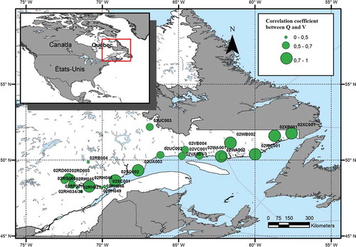
The index-flood model in a multivariate regional FA framework is applied to a regional dataset of interest to the Hydro-Québec Company. The two main flood characteristics, that is, volume V and peak Q are jointly considered. These flood features are random by definition since they are based on the flood start and end dates. The latter are obtained using an automatic method, based on the analysis of cumulative annual hydrographs by adjusting the slopes with a linear approximation (e.g. Ben Aissia et al. 2012). The data employed by Chebana et al. (2009) is from sites in the Côte Nord region in the northern part of the province of Quebec, Canada. The number of sites in the region is N = 26 with record lengths n_i between 14 and 48 years. More information about the data is given in Table 1. Figure 1 presents the geographical location and the correlation coefficient between Q and V for the underlying sites.

Table 1 Discordancy statistic for each site (Chebana et al. 2009).

Site no.	Site name	BV (km^2)	ni	(V,Q) correlation coefficient	Discordancy statistic
					V	Q	(V,Q)
1	Petit Saguenay	729	24	0.50	0.80	0.40	1.09
2	Des Ha Ha	564	19	0.73	3.60	4.44	3.88
3	Aux Écorces	1 120	34	0.5	0.16	2.42	0.69
4	Pikauba	489	34	0.34	0.89	1.16	1.22
5	Métabetchouane	2 270	30	0.54	1.22	1.23	1.59
6	Petite Péribonka	1 090	31	0.62	0.26	0.45	0.98
7	Chamouchouane (Ashuapmushuan)	15 300	43	0.70	0.13	0.14	0.26
8	Mistassibi	8 690	39	0.52	0.32	0.78	0.88
9	Mistassini	9 620	43	0.52	0.62	0.19	0.53
10	Manouane	3 720	23	0.39	0.55	0.47	2.38
11	Valin	740	31	0.42	0.40	0.46	2.37
12	Ste-Marguerite	1 100	21	0.48	1.50	0.55	1.30
13	DesEscoumins	779	19	0.49	1.14	1.81	1.27
14	Portneuf	2 580	20	0.80	0.99	0.32	1.06
15	Godbout	1 570	30	0.75	0.91	0.89	1.29
16	Aux-Pékans	3 390	16	0.54	3.19	0.38	2.25
17	Tonerre	674	48	0.64	0.51	1.65	2.25
18	Magpie	7 200	27	0.66	0.12	1.23	1.11
19	Romaine	13 000	48	0.68	1.62	0.48	0.57
20	Nabisipi	2 060	25	0.78	1.12	0.64	0.54
21	Aguanus	5 590	19	0.60	1.53	0.84	3.07
22	Natashquan	15 600	39	0.75	0.28	0.39	1.02
23	Etamamiou	2 950	19	0.82	1.06	1.33	1.32
24	St Augustin	5 750	14	0.73	0.62	0.67	0.92
25	St Paul	6 630	25	0.73	0.31	1.35	1.11
26	Moisie	19 000	39	0.65	1.16	0.32	0.54

Fig. 1 Geographical chart of the location of the sites.

4.1 Study procedure

The procedure used in the study comprises the following eight steps:

1. Delineate the homogeneous region.

2. Assess the location parameters μ_iV and μ_iQ for i = 1, …, N′ given by equation (13).

3. Select a family of regional multivariate distributions to fit the standardized data of the whole region.

4. For each site in the homogeneous region, estimate the parameters of the marginal distributions and copula family. Estimate the regional parameter estimator by equation (14).

5. Estimate different combinations of the estimated growth curve from equation (12).

6. Estimate the index flood by a multi-regression model from equation (15).

7. Using equation (16), estimate the bivariate regional quantiles associated with the risk p.

8. For each flood characteristic, estimate the univariate regional growth curve and using equation (8), estimate the univariate regional quantile.

9. Evaluate the performance of the regional models (univariate and bivariate) by Monte Carlo simulation.

4.2 Results and discussion

In this section, the results of the application of the adopted procedure are presented. First, the results of the multivariate homogeneity study are briefly presented followed by the results of the index-flood regional estimation.

4.2.1 Discordancy and homogeneity

The employed data are the same as used in Chebana et al. (2009) and the discordancy and homogeneity results are presented in that study and in Table 1. The sites that may be discordant have a large discordancy value. The results show that:

• Sites 2 and 16 are discordant for V;

• Site 2 or sites 2 and 3 are discordant for Q; and

• Sites 2 and 21 are discordant for (V,Q).

The two sites 2 and 21 are eliminated to enable application of the respective homogeneity test. Table 2 presents the homogeneity test values for the region for V, Q and (V,Q) after removing the two discordant sites 2 and 21. From Table 2, according to the statistic H, we conclude that the region is homogeneous for V, heterogeneous for Q and could be homogeneous for (V,Q).

Table 2 Homogeneity after exclusion of the discordant sites.

	V	Q	(V,Q)
H	0.7052	2.4081	1.5234

4.2.2 Identification of marginal distributions

In regional FA, a single frequency distribution is fitted from the whole standardized data. In general, it will be difficult to get a homogeneous region, consequently there will be no single ‘true’ marginal distribution that applies to each site (Hosking and Wallis 1997). Therefore, the aim is to find a marginal distribution that will yield accurate quantile estimates for each site. The scale factor of this marginal distribution changes from one site to another.

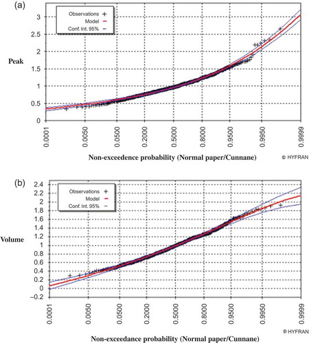
Figure 2 shows that the adequate marginal distributions are Gumbel for Q and GEV for V. Results for the appropriate marginal distributions are in agreement with those of similar studies e.g. Cunnane and Nash (1971) and De Michele and Salvadori (2002).

Fig. 2 Fitting of the marginal distribution of (a) Q and (b) V.

4.2.3 Identification of copula

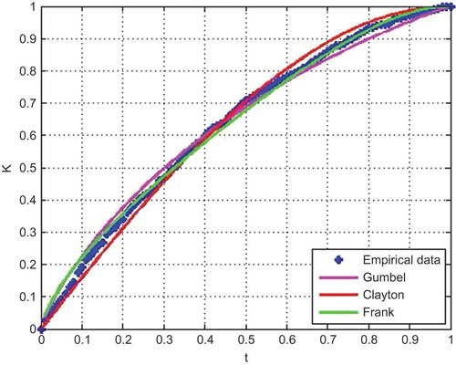
Table 1 indicates that the dependence between V and Q varies from 0.34 to 0.82, while Fig. 1 shows that the dependence variability is scattered over the entire study area. The graphic test based on the K function (5) with the estimate (6) is applied for the three Archimedean copulas: Gumbel, Frank and Clayton. This test leads to fitting the Frank copula to the bivariate data for the studied region. The illustration of this fitting is presented in Fig. 3.

Fig. 3 Copula fitting using K-function.

The AIC and p value of the S_n goodness-of-fit test described earlier and proposed by Kojadinovic and Yan (2011) are also calculated for the commonly considered copulas in hydrology. However, direct results show that none of the commonly used copulas in hydrology can be accepted. Even though the graphic test based on the K function indicates excellent fitting with Frank copula, the S_n goodness-of-fit test rejects this copula, as well as the other ones being considered. First, the reason may be that numerical tests tend to be narrowly focused on a particular aspect of the relationship between the empirical copula and the theoretical copula and often try to compress that information into a single descriptive number or test result (see e.g. NIST 2013). Second, the test is widely and successfully applied to at-site hydrological studies which is not the case for regional studies where the total sample size is very large (here n = 714). The performance of S_n goodness-of-fit test could be affected when the sample size is large, as indicated in Genest et al. (2009). In addition, in terms of application, Vandenberghe et al. (2010) indicated limitations of this test for long sample sizes such as rainfall. Therefore, to overcome this situation, this test is applied to the data series of each site separately. This is justified since regional FA basically assumes the same distribution in each site apart from a scale factor (see e.g. Hosking and Wallis 1997, Ouarda et al. 2008). However, according to Hosking and Wallis (1997), it is difficult in practice to have a single distribution which provides a good fit for each site. The goal is hence to find a distribution that will yield accurate quantile estimates for all sites. The results of our case study (Table 3) show that the Frank copula is the most accepted copula in the study sites (accepted by the S_n goodness-of-fit test for 20 sites and sorted best by AIC for 17 out of 24 sites). The Frank copula has already been shown to be adequate to model the dependence between flood V and Q in a number of hydrological studies (see e.g. Grimaldi and Serinaldi 2006). Finally, based on the above arguments (at-site goodness-of-fit selection, regional graphic test based on the K function, regional and at-site AIC, hydrological literature), the Frank copula is selected for the present case study, defined by:

(23)

where γ is the parameter to be estimated. The choice of the adequate copula is in agreement with those of similar studies, e.g Lee et al. (2013).

Table 3 Results of Sn goodness-of-fit test and AIC criterion for considered copulas. Grey shading indicates that Frank copula is accepted by Sn goodness-of-fit test (p-value column) and has the smallest AIC (AIC column) for the corresponding site.

Site	Gumbel		Frank		Clayton		Galambos		Husler-Reiss		Placket
	p value	AIC	p value	AIC	p value	AIC	p value	AIC	p value	AIC	p value	AIC
1	0.190	−75.0	0.078	−97.5	0.012	−55.2	0.237	−74.5	0.318	−74.1	0.034	−66.6
3	0.086	−106.2	0.081	−151.7	0.175	−72.2	0.095	−105.4	0.117	−104.8	0.086	−86.5
4	0.173	−98.6	0.154	−200.9	0.460	−70.8	0.183	−97.4	0.194	−96.6	0.191	−84.5
5	0.150	−114.0	0.137	−177.7	0.083	−82.3	0.169	−113.2	0.187	−112.4	0.068	−102.6
6	0.128	−146.8	0.133	−103.9	0.064	−102.3	0.030	−146.5	0.028	−145.9	0.044	−131.7
7	0.152	−210.9	0.054	−202.4	0.003	−140.0	0.159	−210.2	0.202	−209.1	0.020	−182.3
8	0.135	−142.9	0.207	−181.7	0.120	−95.0	0.148	−142.1	0.175	−141.3	0.135	−116.7
9	0.148	−175.2	0.404	−231.1	0.041	−115.7	0.155	−174.2	0.197	−173.2	0.214	−145.1
10	0.459	−48.0	0.231	−96.7	0.104	−36.6	0.480	−47.4	0.522	−47.1	0.218	−42.0
11	0.002	−101.2	0.017	−172.8	0.242	−71.4	0.002	−100.3	0.002	−99.5	0.017	−86.5
12	0.120	−66.7	0.113	−59.9	0.200	−48.7	0.114	−66.4	0.112	−66.2	0.180	−58.6
13	0.016	−71.4	0.037	−101.0	0.079	−56.2	0.016	−70.9	0.016	−70.4	0.036	−69.6
14	0.027	−101.0	0.058	24.1	0.019	−78.1	0.026	−101.1	0.029	−101.0	0.020	−98.7
15	0.120	−160.8	0.041	−164.2	0.048	−118.1	0.118	−160.3	0.130	−159.2	0.066	−153.5
16	0.243	−43.0	0.124	−56.0	0.227	−33.1	0.253	−42.7	0.249	−42.5	0.199	−39.1
17	0.048	−164.2	0.003	−230.3	0.000	−113.1	0.059	−163.2	0.069	−162.1	0.003	−143.3
18	0.092	−123.2	0.112	−105.3	0.255	−88.9	0.081	−122.7	0.069	−122.1	0.135	−113.4
19	0.214	−236.0	0.177	−180.7	0.150	−149.6	0.208	−235.3	0.222	−234.4	0.192	−193.7
20	0.352	−122.2	0.326	28.1	0.059	−90.4	0.366	−122.1	0.345	−121.9	0.321	−116.6
22	0.241	−193.4	0.215	−199.3	0.006	−131.4	0.254	−192.7	0.302	−191.6	0.022	−171.5
23	0.002	−100.3	0.011	−184.9	0.040	−85.4	0.002	−100.5	0.007	−101.2	0.002	−104.2
24	0.173	−64.5	0.091	29.3	0.002	−55.0	0.179	−64.5	0.206	−64.6	0.052	−64.8
25	0.138	−107.0	0.310	−111.4	0.031	−78.5	0.140	−106.6	0.140	−106.0	0.035	−99.4
26	0.168	−182.9	0.280	−192.1	0.041	−123.6	0.158	−182.2	0.193	−181.2	0.127	−159.7
Pooled data	0.0005	−329.35	0.045	−365.65	0.0005	−318.94	0.0005	−327.34	0.0005	−300.11	0.04785	−364.86

4.2.4 Estimation of parameters for margins and copula

Parameters of marginal distributions and copula for each site and their corresponding confidence intervals are presented in Fig. 4, while Table 4 gives the regional parameters of the marginal distributions and copula determined by equation (14). The MPL is employed for the copula parameter. For the Gumbel distribution, μ and σ represent, respectively, the location and scale parameters, whereas for the GEV distribution, μ, σ and k represent respectively the location, scale and shape parameters. The ML method is used to estimate the Gumbel parameters, while the generalized ML (Martins and Stedinger 2000) is used to estimate the GEV parameters.

Fig. 4 Parameters of marginal distributions and copula. Dashed lines indicate the confidence interval corresponding to each parameter.

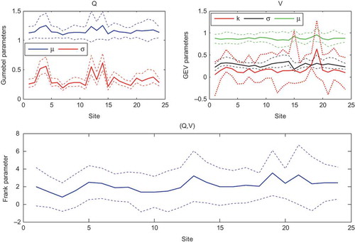
Table 4 Regional parameters of marginal distributions and copula.

Marginal distribution					Copula
Peak (Gumbel)		Volume (GEV)			Frank
μr	σr	kr	σr	μr	γr
1.16	0.33	0.16	0.28	0.88	2.06

4.2.5 Index flood estimation

To estimate the index flood of the peak and of the volume, we use the multi-regression model described by equation (10). The available morphological and climatic characteristics, used as explicative or input variables in the model, are: watershed area, BV (in km²), mean slope of the watershed, BMBV (in %), percentage of forest, PFOR (%), percentage of area covered by lakes, PLAC (%), annual mean of total precipitation, PTMA (in mm), summer mean of liquid precipitation, PLME (in mm), degree days above zero, DJBZ (in °C), absolute value of mean of minimum temperatures in January (Tmin_jan), February (Tmin_feb), March (Tmin_mar) and April (Tmin_apr), absolute value of mean of maximum temperatures in January (Tmax_jan), February (Tmax_feb), March (Tmax_mar) and April (Tmax_apr), and mean of cumulative precipitation in January (PRCP_jan), February (PRCP_feb), March (PRCP_mar) and April (PRCP_apr).

The selection of the significant variables to be included in model (10) is based on the stepwise method. This led to the selection of BV, Tmin_jan, Tmax_fev and PRCP_fev. The model coefficients are estimated by the ML method. Then, the resulting model is given by:

(24)

Note that BV is also selected in similar studies (e.g. Brath et al. 2001), which is not the case for Tmin_jan, Tmax_feb and PRCP_feb.

Model performance is evaluated by the following criteria: coefficient of determination (R^2*), relative root mean square error (RRMSE^*) and mean relative bias (MRB^*) defined by:

(25)

(26)

(27)

where and χ_i represent the estimated and calculated (mean of observed data in subordinate site) index flood respectively, and N' is the number of sites.

The criteria R^2*, RRMSE^* and MRB^* are evaluated on the basis of a cross-validation of the model with the jack-knife method. The results are presented in Table 5. The obtained values of R² are higher than 0.95, which shows high performance of the built model in (10). This performance is confirmed by the low values of RRMSE and MRB in Table 5.

Table 5 Performance criteria of multi-regression index flood model.

	R^2*	MRB^*(%)	RRMSE^* (%)
Q	0.94	1.24	16.75
V	0.97	0.70	11.68

4.2.6 Bivariate and univariate growth curve estimation

The bivariate regional growth curve is estimated for each risk value p by equation (12) and by using the regional parameters of the bivariate distribution. However, univariate regional growth curves of V and Q are estimated directly using regional parameters of marginal distributions. Figure 5 shows the univariate and bivariate estimated growth curves corresponding to non-exceedence probabilities p = 0.9, 0.95, 0.99, 0.995 and 0.999, as well as the quantile curve in the unit square and the marginal distributions for Q and V. Univariate regional growth curves of V and Q are also presented in Table 6. Univariate and bivariate quantiles can be assessed by multiplying growth curves by the corresponding index flood (equation (16)).

Fig. 5 Estimated regional bivariate and univariate growth curves, quantile curve in the unit square and the marginal distributions for Q and V.

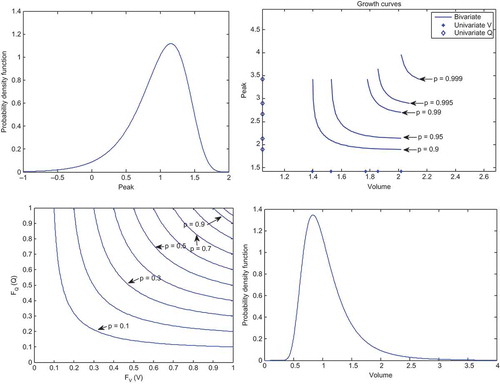
Table 6 Univariate regional growth curve values.

	Marginal distribution	p
		0.9	0.95	0.99	0.995	0.999
Volume	(GEV)	1.40	1.53	1.77	1.85	2.02
Peak	(Gumbel)	1.90	2.13	2.67	2.90	3.43

4.2.7 Model performances

As described above, the accuracy of the quantile estimates of the three regional models: univariate of V (V-model), univariate of Q (Q-model) and bivariate of (V,Q) (VQ-model) is assessed using a Monte Carlo simulation procedure. The record lengths of the simulated sites are assumed to be the same as those of observed data and the number of simulations is set to be M = 500. To illustrate these results, we present in Fig. 6 the univariate and bivariate quantiles of three sites derived from one simulation (M = 1) and from the sample data, as well as quantile curves in the unit square and the local and regional marginal distributions of Q and V. Figure 6 shows that, generally, the performance of the two univariate models and the bivariate model decrease with the risk level and depend on the discordancy values. Indeed, for Mistassibi (Fig. 6(a)) the performance of the V-model is higher than that of the Q-model which is in harmony with the two discordance values of V and Q and with the difference between marginal distributions (local and regional) of Q and V in the side panels. The performance of the bivariate model depends mainly on marginal distributions. Indeed, a small difference in the marginal distribution leads to possible wide shifts in the quantile curve. However, the unit square curves indicate much less effect. Figure 7 illustrates the bivariate quantiles (regional and the 500 simulations) corresponding to a non-exceedence probability of p = 0.9 for the Petit Saguenay station. Figure 7 shows that, in the Petit Saguenay station, the simulated bivariate quantile curves form a surface which includes (but not in the middle) the regional bivariate quantile curve. Table 7 presents the univariate and bivariate model performances of the corresponding non-exceedence probability p = 0.90, 0.95, 0.99, 0.995 and 0.999. The univariate and bivariate model performances at each site are presented in Fig. 8.

Fig. 6(a) Univariate and bivariate quantiles corresponding to a non-exceedence probability p = 0.9, 0.95, 0.99, 0.995 and 0.999 in Mistassibi, quantile curve in the unit square and side panels showing the marginal distributions (local and regional) of Q and V.

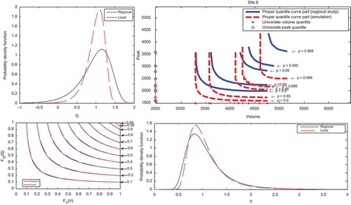
Fig. 6(b) Univariate and bivariate quantiles corresponding to a non-exceedence probability p = 0.9, 0.95, 0.99, 0.995 and 0.999 in Des Escoumins, quantile curve in the unit square and side panels showing the marginal distributions (local and regional) of Q and V.

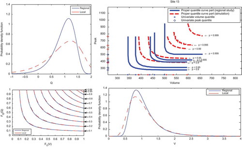
Fig. 6(c) Univariate and bivariate quantiles corresponding to a non-exceedence probability p = 0.9, 0.95, 0.99, 0.995 and 0.999 in Natashquan, quantile curve in the unit square and side panels showing the marginal distributions (local and regional) of Q and V.

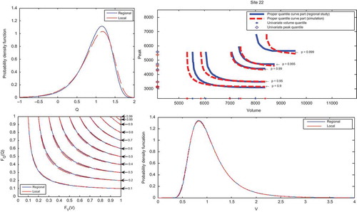
Fig. 7 Bivariate quantiles (Regional and the 500 simulation) corresponding to a non-exceedence probability p = 0.9 in the Petit Saguenay station.

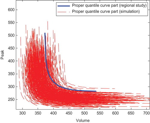
Fig. 8 Performance of the univariate and bivariate quantiles for each site with (a) p = 0.9, (b) p = 0.95, (c) p = 0.99, (d) p = 0.995 and (e) p = 0.999. Continuous line: VQ; dotted line: V and dashed line: Q.

Table 7 Performance of the univariate and bivariate quantiles corresponding to the non-exceedence probabilities 0.9, 0.95, 0.99, 0.995 and 0.999.

Risk	Criterion	(V,Q)	V	Q
p = 0.9	RB	1.99	–1.25	–0.94
	ARB	9.60	3.44	11.87
	RRMSE	15.25	7.68	13.88
p = 0.95	RB	3.27	–1.34	–1.05
	ARB	11.25	4.32	13.56
	RRMSE	17.34	9.37	15.83
p = 0.99	RB	2.49	–0.78	–1.26
	ARB	12.03	5.95	15.99
	RRMSE	17.93	13.56	18.79
p = 0.995	RB	3.41	–0.20	–1.73
	ARB	12.87	7.25	16.93
	RRMSE	19.06	14.90	19.77
p = 0.999	RB	3.23	0.56	–1.51
	ARB	12.21	7.89	18.95
	R^RMSE	18.21	15.79	21.78

Table 7 shows that the V-model performs well, since all performance criteria are less than 16% for all values of p. However, the performance of the Q-model is lower compared to that of the V-model where for instance, for p = 0.999, the RRMSE is larger than 21%. This conclusion can also be drawn from Fig. 8 where the performance criteria of the Q-model are clearly higher than those of the V-model for all values of p. This conclusion can be explained by the fact that the region is heterogeneous for Q. On the other hand, the performance of the VQ-model is, generally, somewhat lower than the Q-model. This conclusion is confirmed by Fig. 8 where we see similar performance criteria for the VQ-model and the Q-model. One can explain this by the fact that the univariate quantiles are special cases of bivariate quantiles, since they correspond to the extreme scenario of the proper part related to the event. Then the performance of the univariate models has an effect on the performance of the bivariate model. Since the performance criteria of the Q-model are higher than those of the V-model, the effect of the Q-model performance on the QV-model is greater than that of the V-model. However, from Fig. 8 we observe that the performance criteria of the VQ-model and the Q-model are similar to those of Gumbel parameters (Fig. 4(a)), especially for the scale parameter (σ). Consequently, a variation of the Gumbel parameters has an effect on the Q-model performance and therefore an effect on the VQ-model performance.

Performance criteria corresponding to the VQ-model are less than 19% for the highest considered risk level, p = 0.999 (Table 7). Values of these performance criteria are larger than those obtained by Chebana and Ouarda (2009). Indeed, unlike their simulation study, the performance of the bivariate model is affected by the error of the index-flood estimation as well as parameter estimations. Generally the performance criteria increase with the value of p (Table 7 and Fig. 8). An exception is recorded between p = 0.995 and p = 0.999, where performance criteria of the VQ-model are higher for p = 0.995. This finding can be explained by the curse of dimensionality in the multivariate context, where the central part of a distribution contains little probability mass compared to the univariate framework (for more details see Scott 1992, Chebana and Ouarda 2009).

In order to further explain the results, we plot in Fig. 9 the RRMSE of each model (for p = 0.99) with respect to the corresponding discordancy values. Ideally we should find an increasing relationship between the RRMSE of each model and the corresponding discordance. This relationship is observed only for the V-model (Fig. 9(a)) since the studied region is homogeneous for V, heterogeneous for Q and could be homogeneous for (V,Q). To find out other factors that have an impact on the model performance, we present in Fig. 10 the RRMSE of the VQ-model (for p = 0.99) with respect to watershed area and the correlation between V and Q. Figure 10(a) shows that high RRMSE values are seen for small watersheds, whereas Fig. 10(b) shows that sites with ρ(V,Q) > 0.6 have a good performance (RRMSE of the order of 10%), with the exception of Godbout (site no. 15), which has ρ = 0.75 and high RRMSE. Godbout is one of the four sites that have a high value of the Gumbel scale parameter and a high RRMSE of the Q-model and the VQ-model.

Fig. 9 RRMSE (%) of the three models with respect to the corresponding discordance values for p = 0.99: (a) margin for V, (b) margin for Q, and (c) bivariate.

Fig. 10 RRMSE of bivariate quantile for p = 0.99 with respect to (a) watershed area (BV) and (b) correlation between V and Q.

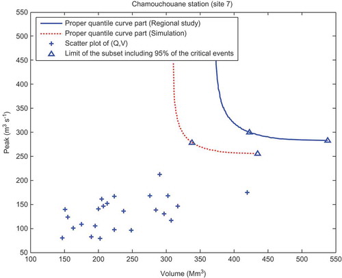
The quantile curve, for a given risk p, leads to infinite combinations of (Q,V) associated with the same return period. However, they could be not equal in practice or from a practical point of view (Chebana and Ouarda 2011). Recently, Volpi and Fiori (2012) proposed a methodology to identify a subset of the quantile curve according to a fixed probability percentage of the events, on the basis of their probability of occurrence; see Volpi and Fiori (2012) for more details. As an illustrative example, the Chamouchouane station is considered. Figure 11 presents the curves and the limits with probability (1 – α) = 0.95.

Fig. 11 Bivariate quantiles of Chamouchouane station corresponding to a non-exceedence probability p = 0.9 with scatter plot of (Q,V) and the limit of subset that includes the critical events with probability (1 – α) = 0.95. Simulation in dotted line and sample data in solid line.

5 CONCLUSIONS AND PERSPECTIVES

The procedure for regional FA in a multivariate framework is applied to a set of sites from the Côte-Nord region in the northern part of the province of Quebec, Canada. This procedure is proposed by Chebana and Ouarda (2009) and represents a multivariate version of the index-flood model. It is based on copulas and multivariate quantiles. Chebana and Ouarda (2009) evaluated the proposed model based on a simulation study. In the present paper, practical aspects of this model are presented and investigated jointly for the flood peak and volume of the considered dataset.

The results show that the appropriate fitted marginal distributions are Gumbel for Q and GEV for V, as well as the Frank copula for their dependence structure. The multi-regressive proposed method to estimate the index flood is shown to lead to a high performance. The performance of the two univariate models is in accordance with the quality of the region (homogeneity test). Indeed, the studied region is homogenous for V and heterogeneous for Q where the performance of the V-model is higher than that of the Q-model. The high performance of the V-model is confirmed by a relationship between their performance criteria and the discordance values of V in each site, whereas the low performance of the Q-model is mainly caused by the variation of the marginal distribution parameters. This is a logical consequence of the heterogeneity of the region for Q. The performance of the two univariate models increases with the risk level p. For the bivariate model, the performance criteria are less than 19% which indicates high performance of the proposed procedure to estimate bivariate quantiles at ungauged sites. This performance increases, generally, with the risk level p and is affected by the performance of the Q-model. The results show also that high values of the performance criteria of the bivariate regional model are seen for small watersheds and for sites with low correlation between V and Q. From this study it is concluded that a good performance of the bivariate model requires good performance of the two univariate models. This means that we should have a homogeneous region for both univariate variables.

The considered method estimates the bivariate quantile as combinations that constitute the quantile curve for a given risk level p. A method to select the appropriate combination(s) for a specific application is of interest and should be developed in future efforts. Furthermore, the adaptation of the model to the estimation of other hydrological phenomena such as drought and the consideration of other homogenous regions can be conducted by considering the appropriate distributions, copulas and events to be studied.

Additional information

Funding

The authors thank the Natural Sciences and Engineering Research Council of Canada (NSERC) and Hydro-Québec for their financial support.

REFERENCES

- Akaike, H., 1973. Information measures and model selection. Information Measures and Model Selection, 50, 277–290.
- Alila, Y., 1999. A hierarchical approach for the regionalization of precipitation annual maxima in Canada. Journal of Geophysical Research D: Atmospheres, 104 (D24), 31645–31655. doi:10.1029/1999JD900764.
- Alila, Y., 2000. Regional rainfall depth-duration-frequency equations for Canada. Water Resources Research, 36 (7), 1767–1778. doi:10.1029/2000WR900046.
- Ashkar, F., 1980. Partial duration series models for flood analysis. Montreal, QC: Ecole Polytech of Montreal.
- Ben Aissia, M.A., et al., 2012. Multivariate analysis of flood characteristics in a climate change context of the watershed of the Baskatong reservoir, Province of Québec, Canada. Hydrological Processes, 26 (1), 130–142. doi:10.1002/hyp.8117.
- Besag, J., 1975. Statistical analysis of non-lattice data. Journal of the Royal Statistical Society. Series D (The Statistician), 24 (3), 179–195.
- Brath, A., et al., 2001. Estimating the index flood using indirect methods. Hydrological Sciences Journal, 46 (3), 399–418. doi:10.1080/02626660109492835
- Burn, D.H., 1990. Evaluation of regional flood frequency analysis with a region of influence approach. Water Resources Research, 26 (10), 2257–2265. doi:10.1029/WR026i010p02257.
- Charpentier, A., Fermanian, J.-D., and Scaillet, O., 2007. The estimation of copulas: theory and practice. New York, NY: Risk Books.
- Chebana, F., et al., 2009. Multivariate homogeneity testing in a northern case study in the province of Quebec, Canada. Hydrological Processes, 23 (12), 1690–1700. doi:10.1002/hyp.7304.
- Chebana, F. and Ouarda, T.B.M.J., 2007. Multivariate L-moment homogeneity test. Water Resources Research, 43 (8). doi:10.1029/2006WR005639.
- Chebana, F. and Ouarda, T.B.M.J., 2009. Index flood-based multivariate regional frequency analysis. Water Resources Research, 45 (10). doi:10.1029/2008WR007490.
- Chebana, F. and Ouarda, T.B.M.J., 2011. Multivariate quantiles in hydrological frequency analysis. Environmetrics, 22 (1), 63–78. doi:10.1002/env.1027.
- Chernick, M.R., 2012. The jackknife: a resampling method with connections to the bootstrap. Wiley Interdisciplinary Reviews: Computational Statistics, 4 (2), 224–226. doi:10.1002/wics.202.
- Cunnane, C. and Nash, J.E., 1971. Bayesian estimation of frequency of hydrological events. In: Mathematical models in hydrology, vol. 1. Proceedings of Warsaw symposium, July 1971. Wallingford, UK: International Association of Hydrological Sciences, IAHS Publ. 100, 47–55.
- Dalrymple, T., 1960. Flood-frequency analyses. Washington, DC: United States Government Printing Office.
- De Michele, C., et al., 2005. Bivariate statistical approach to check adequacy of dam spillway. Journal of Hydrologic Engineering, 10 (1), 50–57. doi:10.1061/(ASCE)1084-0699(2005)10:1(50).
- De Michele, C. and Salvadori, G., 2002. On the derived flood frequency distribution: analytical formulation and the influence of antecedent soil moisture condition. Journal of Hydrology, 262 (1–4), 245–258. doi:10.1016/S0022-1694(02)00025-2.
- Demarta, S. and McNeil, A.J., 2005. The t copula and related copulas. International Statistical Review, 73 (1), 111–129. doi:10.1111/j.1751-5823.2005.tb00254.x.
- Durrans, S.R. and Tomic, S., 1996. Regionalization of low-flow frequency estimates: an Alabama case study. Journal of the American Water Resources Association, 32 (1), 23–37. doi:10.1111/j.1752-1688.1996.tb03431.x.
- Genest, C., Ghoudi, K., and Rivest, L.-P., 1995. A semiparametric estimation procedure of dependence parameters in multivariate families of distributions. Biometrika, 82 (3), 543–552. doi:10.1093/biomet/82.3.543.
- Genest, C., Rémillard, B., and Beaudoin, D., 2009. Goodness-of-fit tests for copulas: a review and a power study. Insurance: Mathematics and Economics, 44 (2), 199–213.
- Genest, C. and Rivest, L.-P., 1993. Statistical inference procedures for bivariate archimedean copulas. Journal of the American Statistical Association, 88 (423), 1034–1043. doi:10.1080/01621459.1993.10476372.
- GREHYS, 1996a. Presentation and review of some methods for regional flood frequency analysis. Journal of Hydrology, 186 (1–4), 63–84. doi:10.1016/S0022-1694(96)03042-9.
- GREHYS, 1996b. Inter-comparison of regional flood frequency procedures for Canadian rivers. Journal of Hydrology, 186 (1–4), 85–103. doi:10.1016/S0022-1694(96)03043-0.
- Grimaldi, S. and Serinaldi, F., 2006. Asymmetric copula in multivariate flood frequency analysis. Advances in Water Resources, 29 (8), 1155–1167. doi:10.1016/j.advwatres.2005.09.005.
- Hamza, A., et al., 2001. Développement de modèles de queues et d’invariance d’échelle pour l’estimation régionale des débits d’étiage. Canadian Journal of Civil Engineering, 28 (2), 291–304. doi:10.1139/l00-121.
- Hosking, J.R.M. and Wallis, J.R., 1993. Some statistics useful in regional frequency analysis. Water Resources Research, 29 (2), 271–281. doi:10.1029/92WR01980.
- Hosking, J.R.M. and Wallis, J.R., 1997. Regional frequency analysis: an approach based on L-moments. Cambridge: Cambridge University Press.
- Kim, J.-M., et al., 2008. A copula method for modeling directional dependence of genes. BMC Bioinformatics, 9 (1), 225. doi:10.1186/1471-2105-9-225.
- Kim, G., Silvapulle, M.J., and Silvapulle, P., 2007. Comparison of semiparametric and parametric methods for estimating copulas. Computational Statistics and Data Analysis, 51 (6), 2836–2850. doi:10.1016/j.csda.2006.10.009.
- Kojadinovic, I. and Yan, J., 2011. A goodness-of-fit test for multivariate multiparameter copulas based on multiplier central limit theorems. Statistics and Computing, 21 (1), 17–30.
- Lee, T., Modarres, R., and Ouarda, T.B.M.J., 2013. Data based analysis of bivariate copula tail dependence for drought duration and severity. Hydrological Processes, 27 (10), 1454–1463.
- Martins, E.S. and Stedinger, J.R., 2000. Generalized maximum-likelihood generalized extreme-value quantile estimators for hydrologic data. Water Resources Research, 36 (3), 737–744. doi:10.1029/1999WR900330.
- Meng, X.L. and Rubin, D.B., 1993. Maximum likelihood estimation via the ECM algorithm: a general framework. Biometrika, 80 (2), 267–278. doi:10.1093/biomet/80.2.267.
- Nelsen, R.B., 2006. An introduction to copulas. New York: Springer.
- Nezhad, M.K., et al., 2010. Regional flood frequency analysis using residual kriging in physiographical space. Hydrological Processes, 24 (15), 2045–2055.
- Nguyen, V.-T.-V. and Pandey, G. (1996). A new approach to regional estimation of floods in Quebec. In: Proceedings of the 49th annual conference of the CWRA. Collection Environnement de l’Université de Montréal: Quebec City, 587–596.
- NIST (2013). e-Handbook of Statistical Methods. Available from: http://www.itl.nist.gov/div898/handbook/pmd/section4/pmd44.htm [Accessed September 2013].
- Ouarda, T.B.M.J., et al., 2000. Regional flood peak and volume estimation in northern Canadian basin. Journal of Cold Regions Engineering, 14 (4), 176–191. doi:10.1061/(ASCE)0887-381X(2000)14:4(176).
- Ouarda, T.B.M.J., et al., 2001. Regional flood frequency estimation with canonical correlation analysis. Journal of Hydrology, 254 (1–4), 157–173. doi:10.1016/S0022-1694(01)00488-7.
- Ouarda, T.B.M.J., et al., 2006. Data-based comparison of seasonality-based regional flood frequency methods. Journal of Hydrology, 330 (1–2), 329–339. doi:10.1016/j.jhydrol.2006.03.023.
- Ouarda, T.B.M.J., et al., 2008. Intercomparison of regional flood frequency estimation methods at ungauged sites for a Mexican case study. Journal of Hydrology, 348 (1–2), 40–58. doi:10.1016/j.jhydrol.2007.09.031.
- Pilon, P.J., 1990. The Weibull distrubution applied to regional low-flow frequency analysis. In: A. Beran et al., eds., Regionalization in hydrology. (Proceedings of the Ljubljana symposium) Wallingford, UK: International Association of Hydrological Sciences, IAHS Publ. 191, 227–237.
- Rencher, A.C., 2003. Methods of multivariate analysis. New York: John Wiley & Sons. doi:10.1002/0471271357.
- Salvadori, G., et al., 2007. Extremes in nature: an approach using copula. Berlin: Springer, p. 292.
- Schwarz, G., 1978. Estimating the dimension of a model. Annals of Statistics, 6 (2), 461–464. doi:10.1214/aos/1176344136.
- Scott, D.W., 1992. Multivariate density estimation: theory, practice, and visualization. New York: Wiley.
- Shiau, J.T., 2003. Return period of bivariate distributed extreme hydrological events. Stochastic Environmental Research and Risk Assessment (SERRA), 17 (1–2), 42–57. doi:10.1007/s00477-003-0125-9.
- Shih, J.H. and Louis, T.A., 1995. Inferences on the association parameter in copula models for bivariate survival data. Biometrics, 51 (4), 1384–1399. doi:10.2307/2533269.
- Singh, V.P., 1987. Regional flood frequency analysis. Dordrecht: D. Reidel.
- Sklar, A., 1959. Fonction de répartition à n dimensions et leurs margins. Institut Statistique de l’Université de Paris, 8, 229–231.
- Stedinger, J.R. and Tasker, G.D., 1986. Regional hydrologic analysis, 2, model-error estimators, estimation of sigma and log-Pearson type 3 distributions. Water Resources Research, 22 (10), 1487–1499. doi:10.1029/WR022i010p01487.
- Vandenberghe, S., Verhoest, N.E.C., and De Baets, B., 2010. Fitting bivariate copulas to the dependence structure between storm characteristics: a detailed analysis based on 105 year 10 min rainfall. Water Resources Research, 46 (1), W01512. doi:10.1029/2009WR007857.
- Volpi, E. and Fiori, A., 2012. Design event selection in bivariate hydrological frequency analysis. Hydrological Sciences Journal, 57 (8), 1506–1515. doi:10.1080/02626667.2012.726357.
- Wiltshire, S.E., 1987. “Statistical techniques for regional flood-frequency analysis. [electronic resource].”
- Yue, S., 2001. A bivariate extreme value distribution applied to flood frequency analysis. Nordic Hydrology, 32 (1), 49–64.
- Yue, S., et al., 1999. The Gumbel mixed model for flood frequency analysis. Journal of Hydrology, 226 (1–2), 88–100. doi:10.1016/S0022-1694(99)00168-7.
- Zhang, L. and Singh, V.P., 2006. Bivariate flood frequency analysis using the copula method. Journal of Hydrologic Engineering, 11 (2), 150–164. doi:10.1061/(ASCE)1084-0699(2006)11:2(150).
- Zhang, L. and Singh, V.P., 2007. Trivariate flood frequency analysis using the Gumbel-Hougaard copula. Journal of Hydrologic Engineering, 12 (4), 431–439. doi:10.1061/(ASCE)1084-0699(2007)12:4(431).