Modelling long-term water yield effects of forest management in a Norway spruce forest

Abstract

Intensive forest management is one of the main land cover changes over the last century in Central Europe, resulting in forest monoculture. It has been proposed that these monoculture stands impact hydrological processes, water yield, water quality and ecosystem services. At the Lysina Critical Zone Observatory, a forest catchment in the western Czech Republic, a distributed physics-based hydrologic model, Penn State Integrated Hydrologic Model (PIHM), was used to simulate long-term hydrological change under different forest management practices, and to evaluate the comparative scenarios of the hydrological consequences of changing land cover. Stand-age-adjusted LAI (leaf area index) curves were generated from an empirical relationship to represent changes in seasonal tree growth. By consideration of age-adjusted LAI, the spatially-distributed model was able to successfully simulate the integrated hydrological response from snowmelt, recharge, evapotranspiration, groundwater levels, soil moisture and streamflow, as well as spatial patterns of each state and flux. Simulation scenarios of forest management (historical management, unmanaged, clear cutting to cropland) were compared. One of the critical findings of the study indicates that selective (patch) forest cutting results in a modest increase in runoff (water yield) as compared to the simulated unmanaged (no cutting) scenario over a 29-year period at Lysina, suggesting the model is sensitive to selective cutting practices. A simulation scenario of cropland or complete forest cutting leads to extreme increases in annual water yield and peak flow. The model sensitivity to forest management practices examined here suggests the utility of models and scenario development to future management strategies for assessing sustainable water resources and ecosystem services.

Editor D. Koutsoyiannis

Résumé

La gestion intensive des forêts a induit l’un des principaux changements d’occupation des sols au cours du siècle dernier en Europe centrale, résultant en une monoculture forestière. Ces peuplements monospécifiques ont été proposés pour influencer les processus hydrologiques, le rendement en eau, la qualité de l’eau et les services écosystémiques. A l’Observatoire de la zone critique de Lysina, qui est un bassin versant forestier situé dans la partie occidentale de la République tchèque, un modèle hydrologique distribué fondé sur la physique, le modèle hydrologique intégré de l’Etat de Pennsylvanie (PIHM), a été utilisé pour simuler l’évolution hydrologique à long terme dans le cadre des pratiques de gestion forestière, et pour évaluer des scénarios comparatifs des conséquences hydrologiques de changement d’occupation des sols. Des courbes d’indices foliaires (leaf area index – LAI) ajustés selon l’âge des parcelles ont été générées à partir d’une relation empirique pour représenter les changements de la croissance saisonnière des arbres. En considérant le LAI ajusté selon l’âge, le modèle spatialement distribué a été capable de bien simuler la réponse hydrologique intégrée de la fonte des neiges, de la recharge, de l’évapotranspiration, des niveaux de l’eau souterraine, de l’humidité du sol et du débit, ainsi que la répartition spatiale de chaque état et flux. Les scénarios de simulation de gestion forestière (gestion historique, absence de gestion, coupe à blanc) ont été comparés. L’une des conclusions essentielles de l’étude suggère que la coupe sélective (par lot) de la forêt montre une augmentation légère du ruissellement (rendement en eau) par rapport au scénario simulé d’absence de gestion (pas de coupe) sur une période de 29 ans à Lysina, indiquant que le modèle est sensible aux pratiques de coupe sélective. Un scénario de simulation de terres arables ou de coupe forestière complète conduit à des augmentations énormes du rendement annuel en eau et du débit de pointe. La sensibilité du modèle aux pratiques de gestion forestière examinées ici souligne l’utilité de développer des modèles et des scénarios pour évaluer des ressources en eau et des services écosystémiques durables dans le cadre de futures stratégies de gestion.

Key words:

• Lysina Critical Zone Observatory
• PIHM
• Norway spruce
• forest management

Mots clefs:

• Observatoire de la zone critique de Lysina
• PIHM
• épicéa de Norvège
• gestion de forêt

1 INTRODUCTION

Catchment hydrological behaviour has important linkages and feedbacks that influence forest growth and health, although spatially-distributed quantitative hydrological assessments are rarely available due to the lack of detailed data for the hydrology, climate, forest management and geological setting. Qualitatively, we know that water consumption by trees is integrated with atmospheric and climatic conditions and subsurface moisture storage, while excess precipitation beyond that utilized by trees will support surface runoff or will infiltrate and return to streams as baseflow. Processes of canopy interception, throughfall, snowmelt and land surface evaporation also play important roles in the circulation of water in forested catchments. It has even been suggested that forest management increases the complexity of hydrological processes in forested catchments by amplifying certain of these components at the expense of others (Eisenbies et al. 2007, Vanclay 2009).

Experimental studies to assess the hydrological impact on forested catchments have often been conducted using paired catchments. The approach has been applied worldwide to assess the effects of vegetation change on water yield since the beginning of the 20th century (John and Hibbert 1961, Hornbeck et al. 1993, Stednick 1996). The role of forest management in watershed hydrology has been the subject of several discussion papers and review articles (e.g. Bosch and Hewlett 1982, Stednick 1996, Andréassian 2004, Brown et al. 2005). The general conclusions are that paired catchment experiments can qualitatively explain annual water yield differences; however, spatial details of hydrological forest management practices on hydrological flow patterns are difficult to assess quantitatively with this approach. Spatially-distributed hydrologic models provide an independent means of evaluating the impact of managed land-cover changes on water resources within a catchment. Hydrologic modelling studies explicitly driven by land-cover change scenarios offer a quantitative approach to assessing the impact of forest management on hydrological processes (Eisenbies et al. 2007, Thanapakpawin et al. 2007, Wijesekara et al. 2012).

Soil–vegetation–atmosphere transfer schemes in general circulation models (GCMs) are now widely used to assess large-scale hydrological impacts of forest management. The strategy provides an integrated response of vegetation water use for a GCM grid cell using leaf surface area to scale land surface energy and water budgets, including the functions of soil moisture (Arora 2002). Wattenbach et al. (2007) simulated the annual sub-grid water balance and seasonal pattern of impacts using the percentage of afforestation. Wijesekara et al. (2012) linked a land-use change model to a physically-based distributed model and predicted hydrological responses to the percentage of each land-use type. Studies have found that considerable variation in the hydrological regime occurs as the forest stand ages (Murakami et al. 2000, Kostner et al. 2002). However, it has also been argued that the percentage of forest cover alone is not a sufficient measure to analyse and model the derived watershed-scale hydrology without considering the growth condition of the forest (Andréassian 2004). Currently, most hydrological models do not parameterize vegetation as a dynamic component, and thus the importance of ecohydrological function of forests on catchment hydrology is often missing in water balance studies (Arora 2002, Wattenbach et al. 2005).

In Central Europe, intensive forest management has resulted in large areas of forest monoculture, largely driven by economic benefits. A typical case is stands of Norway spruce (Picea abies) that were planted outside their natural range, displacing native European beech (Fagus sylvatica) species (Ellenberg 1996). Such activities have induced considerable hydrological impacts. Paired or controlled catchment studies suggested that the hydrological impacts of monoculture forests are sensitive to soil and forest type (Robinson et al. 2003, van Dijk and Keenan 2007).

Recently, the European Union initiated a programme of research using Earth’s Critical Zone Observatories (CZOs) (Banwart et al. 2011). The Lysina CZO is an experimental catchment to study the resilience of soil functions to acid deposition and other impacts in a heavily managed forest catchment used for timber production. Under the outline of the research framework of European CZOs (Banwart et al. 2012), an effort was undertaken to compile and digitize extensive historical forest management data of stand age, soil and hydrogeological characterization within a mathematical modelling framework for the Lysina catchment. The aim of this study was to test how well a physics-based, meso-scale distributed model, PIHM (Penn State Integrated Hydrologic Model; Qu and Duffy 2007, Kumar 2009), can simulate the intensive management practices and impacts on hydrological processes at the Lysina catchment using a simple representation of the historical record of forest growth based on biomass and leaf area index (LAI). Here PIHM is referred to as a meso-scale model with mesh sizes intermediate to plot- or micro-scale models (Dooge 1988) and regional-scale climate or ecohydrology models. Using PIHM allowed the spatial structure of forest management units within the watershed to have independent growth (LAI) histories. The average mesh size in this case is around 20 metres. Calibration and validation of the model for the entire watershed was constrained by observed streamflow at the outlet, groundwater levels at several monitoring sites and the historical LAI/growth history information for each management unit. Climate/weather forcing was available at two nearby stations. Once implemented, model evaluations of past scenarios allow the quantitative assessment of hydrological impacts of management practices, while providing a reference for future logging and replanting plans, and assessment of Critical Zone (CZ) evolution under environmental changes. We expect that the spatially-distributed model will be a useful tool for assessing future water resources and water quality under changing climate and management conditions.

2 SETTING AND STRATEGY

2.1 Lysina watershed

Lysina is a well-documented catchment with long-term forest management and environmental monitoring records. The 29.3-ha headwater catchment is located at 50°03′N, 12°40′E in the western part of the Czech Republic (Fig. 1), within a large spruce forest on the plateau of the Slavkov Forest (Slavkovský les), a protected mountainous region with an area of 610 km². Lysina catchment has been continuously monitored since 1989, with the primary focus on the effects of anthropogenic atmospheric deposition on stream water chemistry (Krám et al. 1995, 1997, Hruška et al. 2009). The study site belongs to the Czech Republic national network GEOMON (GEOchemical MONitoring) of small forest catchments (Oulehle et al. 2008), and the Lysina catchment is one of two Czech sites within the international network of forest sites comprising the International Cooperative Program – Integrated Monitoring (Holmberg et al. 2013), organized under the Economic Commission for Europe of the United Nations. The Lysina catchment also belongs to the Long-Term Ecosystem Research (LTER) network and recently became one of the European CZOs within the SoilTrEC (Soil Transformations in European Catchments) project (Banwart et al. 2011, 2012).

Fig. 1 (a) Lysina catchment sites I and II each have two piezometers. Topographic contours are shown at 1-m intervals. (b) Two Czech Hydrometeorological Institute (CHMI) weather stations were available at Lazy and Mariánské Lázn (ML). (c) Location of the Lysina catchment.

The climate at Lysina is classified as temperate continental, with relatively hot summers and cold, cloudy and snowy winters. The mean annual temperature of the nearest meteorological station (Mariánské Lázně) was 6.0°C (range: 4.5–7.1°C) and the mean annual precipitation was 834.5 mm year^-1 (range: 523.4–1165.4 mm year^-1) during the period 1967–2011, as shown in Fig. 2. In spite of plentiful summer precipitation, winter runoff volume forms the major part of annual runoff. The topography at Lysina is comprised of low hills with an average slope of 11.5% and a northeast orientation. The elevation ranges from 829 to 949 m a.s.l. The prevailing soils are gleysols (52%) and podzols (41%), along with occasional peaty soil (6%), rankers (1%) and rock outcrops with no soil development (0.3%). The soil map of Lysina catchment has been digitized using the modified information from the UHUL (the Forest Management Institute of the Czech Republic), Brandýs nad Labem, branch Karlovy Vary (Fig. 3).

Fig. 2 (a) Annual temperature and precipitation at the base climate station (ML; elevation 691 m). (b) Monthly mean temperature, precipitation and runoff during the last two decades (1990–2011) at climate station ML. (c) Scatterplot of monthly precipitation at raingauges ML and Lazy, from 2006 to 2011.

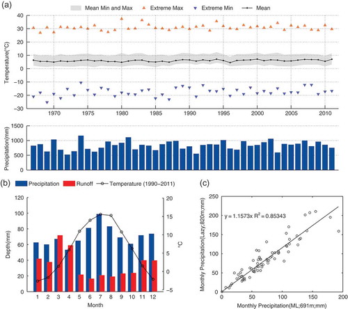
Fig. 3 Soil map of the Lysina catchment. The prevailing soils are gleysol (52%) and podzol (41%); three more soil types are present: peaty soil (6%), ranker (1%) and not developed soil on rock outcrops (0.3%).

2.2 Field measurement and data collection

Precipitation, air temperature, wind speed, relative humidity and global radiation were measured by the national meteorological service, the Czech Hydrometeorological Institute (CHMI), using the standard meteorological station at Mariánské Lázně (ML) (691 m a.s.l., 49°59′N, 12°42′E) located approx. 5 km from Lysina (Fig. 1). The data were available at hourly intervals with the exception of global radiation (daily sum) for the period 2006 to present. Historical data were available at daily time steps since 1967. Another source of precipitation data is from the raingauge station at Lazy (820 m a.s.l., 50°2′N, 12°22′E) approx. 3 km from Lysina, which better represents the local catchment conditions than the meteorological station at ML (Fig. 1). Due to the strong correlation of monthly precipitation between ML and Lazy (Fig. 2(c)), we calculated the precipitation–elevation gradient (1.35 mm year^-1 m^-1) to estimate precipitation at Lysina. The meteorological forcing data were assumed to be spatially uniform across the 29.3-ha catchment.

A float-operated OTT Thalimedes shaft encoder with integral data logger measured streamgauge heights above a V-notch weir at 20-min intervals at the watershed outlet. The streamflow was calculated using a standard rating curve method developed for the weir. The 20-min discharge values were aggregated to hourly and daily runoff in cubic metres.

Groundwater patterns were monitored in five piezometers by manual measurements at weekly intervals from September 2011. The piezometers are located at three different places, two in pairs and one single piezometer (Fig. 1). The depths of piezometers Ia and Ib are 3.58 and 3.92 m below ground surface (b.g.s.); those of IIa and IIb are 1.2 and 2.59 m b.g.s.; and that of IV is 2.89 m b.g.s; the latter site is just outside the watershed. Observation well lithology was used to estimate the lower bound of active groundwater flow.

Daily snow depth observations were collected from ML. The snow water equivalent (SWE) was estimated using the equation from Jonas et al. (2009). The SWE was used for the melt factor calibration:

(1)

where SWE is in kg/m², and HS is snow depth in m.

2.3 Geospatial watershed information

Topography was obtained from a traditional topographic survey done in 1989 with 1 m contours and a final map scale of 1:1000. These data were digitized and converted to a 1-m resolution digital elevation model (DEM), and then the DEM was updated with recent data. In 2003, the location of paths and roads were confirmed by comparison with aerial photos. The stream channels were also surveyed, including the left and right streambank and bed elevation, in 2011.

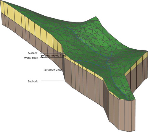
The high-resolution DEM was used for watershed delineation and stream definition as well as to constrain the unstructured mesh and model domain. The domain decomposition (watershed and stream delineation, mesh generation, etc.) was carried out with PIHMgis, a ‘tightly-coupled’ GIS interface to PIHM (Bhatt 2012, Bhatt et al. 2014). The channels were classified as natural or artificial drainage (Fig. 1). The estimated length of all stream channels determined from a topographic survey was 2774 m including 1757 m of ditches. The stream channel network was simplified for the present modelling purposes to a mainstem length of 1045 m including 260 m of the active artificial channels (field inspection). The numerical mesh consisted of 455 irregular triangles and 37 stream segments (Fig. 4). The depth of groundwater flow was estimated from the borehole data to be approx. 4 m below the land surface and this was used in the model.

Fig. 4 Mesh and boundary of the Lysina catchment model. The elevation of the lower limit of impermeable bedrock was set to a uniform 4 m below the surface. The groundwater flow in the catchment is within the soil (0–1.5 m) and weathered bedrock (1.5–4 m). Solid (blue) lines represent the stream channels, and (green) triangles represent the catchment domain.

2.4 Forest management history

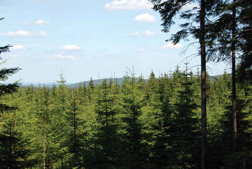
Prior to the spruce monoculture forest, Lysina catchment was a mixed forest comprised of European beech (Fagus sylvatica), Norway spruce (Picea abies) and silver fir (Abies alba) stands (Krám et al. 1999, Hruška and Krám 2003). Intensive forest cutting started around 1520 due to the demand for wood products, especially associated with tin mines at Horní Slavkov, and remained active although erratic until the end of the 18th century. In the middle of the 19th century, many waterlogged areas were drained and systematic silvicultural management started. Around 1850, the first generation of fast growing stands of Norway spruce were planted to increase timber production and to stabilize the forest landscape. Timber was harvested at a later age than previous practices. At the so-called rotation age of 100–130 years, even-aged stands were harvested, with areas of one or more hectares clear-cut. Silvicultural management at Lysina in the 20th century was based entirely upon cutting around 5 ha of even-aged spruce stands until the 1970s, and relatively small units (up to 2 ha) to the present. This type of block cutting produces an uneven age distribution of the forest and limits adverse effects of large-scale single-age timber management such as soil erosion and lost ecosystem services (Swanson and Dyrness 1975). Soon after harvesting, spruce seedlings were planted. Trees are almost always cut after the rotation age following the Czech Forest Law (approx. 100 years for Norway spruce), although harvesting may be accelerated due to the poor health of trees (Krám et al. 1999) due to wind damage, snow damage, bark beetle attack, acid rain or ozone injuries. Figure 5 is a photograph of typical multi-age forest in the Slavkov Forest.

Fig. 5 A photograph taken in the Lysina catchment shows a boundary between the two even-aged Norway spruce stands.

The Czech forest administration produces a forest age/growth map every 10 years to record actual species composition, forest age and biomass stock. These maps were available from 1984 and 2004, along with aerial photographs from 1953, 1969 and 1991. For this research these documents and maps provided the geospatial forest growth history of the Lysina catchment. In 1953, 80% of the catchment was covered by mature trees, approx. 100-year-old spruce forest, while the remaining 20% was covered by young spruce (0–20 years old). In 1969, mature forest covered about 60% of the catchment, 20% was covered by 20–40-year-old spruce forest, and the rest of the catchment was covered by young spruce (0–20 years old). In 1984 approximately 30% of the 100-year-old trees were logged, and the areas replanted with spruce. In 1994, 90% of the trees older than 100 years were harvested, and the areas replanted with young spruce plantation. Forest stands at Lysina (Table 1) represented typical central European mountainous managed forest. The rooting zone of spruce trees is extremely shallow. The majority of the roots are situated in the organic horizon, immediately above the nutrient-poor eluvial horizon.

Table 1 Stand characteristics for Norway spruce at Lysina catchment (unpublished data from the Forests of the Czech Republic, State Co. and Černý et al. 1996).

Age	Tree density	Mean tree height	Basal area	BHD*	Biomass volume
years	(individuals/ha)	(m)	(m^2/ha)	(cm)	(m^3)
10	4500	2	n.d	n.d	n.d.
20	4000	5	n.d	n.d	n.d.
30	3016	8	17.4	8.6	84
40	2396	11.3	25.3	11.6	163
50	1854	14.4	31.4	14.7	246

*BDH: breast high diameter; n.d.: not determined.

Table 2 Model evaluation criteria for the calibration and validation period.

	Calibration (2006)			Validation (2007–2011)
	E (%)	R	NSE	E (%)	R	NSE
Snow water equivalent	4.3	0.96	0.87	8.2	0.86	0.67
Streamflow	3.9	0.93	0.86	4.2	0.79	0.62
	Calibration Site I			Calibration Site II
	E (%)	R	NSE	E (%)	R	NSE
Groundwater-table depth	6.3	0.95	0.66	0.2	0.87	0.76

Important to this study is that the existing empirical data show the relationship of stand age with leaf area, transpiration and biomass (Kostner et al. 2002, Spinnler et al. 2002, Pokorný et al. 2008). Using this published data allowed us to crudely estimate the historic vegetation growth dynamics, by developing regression equations for LAI (leaf area index) and age according to field observations (Fig. 6):

(2)

where maxLAI is annual maximum LAI (m² m^-2), and age is in years. Thus the model adjusted the seasonal LAI curves based on equation (2) for all forest stands.

Fig. 6 Relationship of tree age to leaf area index. ‘+’ represents data from (Spinnler et al. 2002), ‘×’ data from (Kostner et al. 2002), and ‘o’ data from (Pokorný et al. 2008).

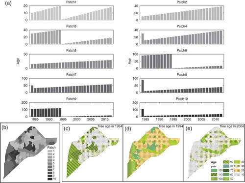
According to the forest management history (Pokorný et al. 2008) and tree age maps of 1984 and 2004 (Czech forest administration), selective cutting management for the watershed was divided into 10 patches representing stands with unique plantation histories (Fig. 7). It is worth mentioning that Czech forest management is usually very continuous, and cutting of young trees rarely happens. Here, the deduced selective cutting history is intended for conducting a comparative study and might not be precise enough at the scale of an individual tree. From this map, reconstructed annual LAI curves modified by stand age were determined for each of the 10 management patches and then projected onto the model domain triangles for the simulation period 1984–2012.

Fig. 7 (a) The rotation management represented by different practices on 10 patches: the bars show the tree age variation on each patch. (b) Patch location in the watershed; (c), (d) and (e) the tree age distribution before management practices in 1984, 1994, 2004, respectively.

2.5 The Penn State Integrated Hydrologic model (PIHM)

The PIHM is a physics-based fully-coupled hydrologic model. It simulates interception, throughfall, infiltration, recharge, evapotranspiration, overland flow, subsurface flow and channel routing in a fully coupled scheme for multi-scale distributed hydrological simulations (Qu and Duffy 2007). The resolution of the triangular mesh is automatically fitted to the terrain with user-constraints to follow geomorphological or hydrological boundaries of the watershed, and triangles can also be constrained by point observations (e.g. streamflow, groundwater level, soil moisture, LAI) and the watershed boundary conditions (Kumar et al. 2009). The model resolves hydrological processes for land surface energy, overland flow, channel routing and subsurface flow, governed by partial differential equations. The system is discretized by the triangular mesh and projected as a volumetric prism from canopy to bedrock (Qu and Duffy 2007). The model also includes canopy interception, evapotranspiration (ET), snow accumulation, snowmelt, infiltration and recharge within the fully-coupled system. The PIHM uses a semi-discrete finite-volume formulation for solving the system of coupled PDEs, resulting in a system of ordinary differential equations (ODE) representing all processes within the prismatic control volume. The local system is assembled throughout the entire model domain and the global ODE system is solved using the CVODE implicit solver (Cohen et al. 1996).

2.6 Model parameter estimation

Calibration of parameters is based on the partition calibration strategy and evolutionary algorithm (Yu et al. 2013). The initial soil and subsurface hydrologic parameters were estimated based on soil textural properties (Wösten et al. 2001). The hydrologic parameters were then optimized through an evolutionary algorithm (Yu et al. 2013) using streamflow observation data from several precipitation events during the spring of 2006. Snow accumulation and melting processes were determined by the temperature index model, where melting rate is a product of melt factor (MF, seasonal variable) and positive air temperature (Kumar 2009). The melt factor is adjusted to match the simulated SWE to the SWE estimated from snow depth observations. Energy parameter estimation (Yu et al. 2013) is based on seasonal LAI, air temperature, relative humidity and wind data for the year 2006. The spatial groundwater table was matched by locally nudging soil hydraulic parameters and soil porosity to match the field data.

3 RESULTS AND DISCUSSION

As an integrated model, PIHM simulated results were compared with multiple observed variables, including SWE, streamflow and groundwater table depth. We used the relative error (E), Pearson product-moment correlation coefficient (R), and Nash-Sutcliffe coefficient of efficiency (NSE) (Nash and Sutcliffe 1970) to evaluate the model performances (Table 1). These criteria are defined as follows:

(3)

(4)

(5)

where t is the total number of time steps in the evaluation period, O is the observed value, and P is the predicted value.

3.1 Snow accumulation and melt processes

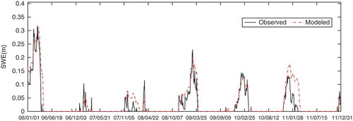
The default MF (melt factor) in PIHM is constructed using sinusoidal interpolation between a minimum value on 21 December (0.6 mm °C^-1 (6 h)^-1) and a maximum value on 21 June (1.2 mm °C^-1 (6 h)^-1) (Anderson 1973). The site specific calibrated MF results were 0.27 (min) and 0.72 (max) mm °C^-1 d^-1, which were smaller than the results in degree-day factor (DDF) model studies (Hock 2003). The simulated SWE agreed with the estimated SWE from snow depth observation in most years (Fig. 8, Table 2), except the spring melt years of 2008 and 2011 when the fit is poorer but still satisfactory for scenario development.

Fig. 8 Comparison between observed and modelled snow water equivalent (SWE) for the period 2006–2011. Observed SWE was estimated from snow depth.

3.2 Streamflow

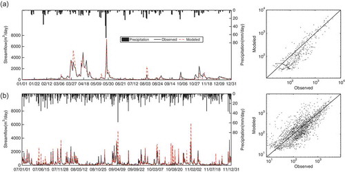
Agreement between modelled and measured daily streamflow indicated satisfactory performance of PIHM for the seasonal water yields of the Lysina catchment over the 2006 calibration period (Fig. 9, Table 2). Comparison of simulated and observed hydrographs shows that the spring snowmelt runoff events were adequately simulated in the model. The summer drought was also well represented in the simulation responding to the overall vegetation water use.

Fig. 9 Comparison between observed and modelled daily streamflow: (a) calibration period (2006); (b) validation period (2007–2011).

3.3 Groundwater

Despite the short period of groundwater observations, the results showed significant differences in groundwater level fluctuations between the sites. Piezometers Ia and Ib, located in the same grid cell, show a similar groundwater table pattern with the lowest elevation in autumn (September and October) and high water levels after snowmelt (April). The water level range for the period was 0.8 m and the average depth to the water table was 1.5 m b.g.s. (Fig. 10). The groundwater levels in IIa and IIb were also located in a single grid cell. The records were averaged since they show the same seasonal trend but with an offset of approx. 1 m of depth to groundwater. The averaged data and model results (Fig. 10) had a below ground depth depth of around 1–2 m. The shallowest depth to groundwater in the model occurred for gleysols (higher clay content). The model-simulated groundwater table elevations were consistent with observations (Table 2).

Fig. 10 Modelled and observed groundwater table depth below surface in 2012: (a) Site Ia and Ib piezometers were located in the same mesh triangle. (b) Site IIa and IIb piezometers were also located in the same grid cell and show the same trend, but with an elevation difference of ~1 m, so the data were averaged and then compared with the model result for the corresponding triangle. The x-axis values are in date format: mm/dd.

3.4 Sources of errors

3.4.1 Uncertainty in meteorological forcing

In Fig. 2(c) the precipitation difference between Lazy and ML represents one source of uncertainty. Significant differences between the sites are found in monthly precipitation during the wet season. Both the timing and magnitude of precipitation input errors in the model could influence the uncertainty of runoff simulation. However, our study is meant to be comparative and as the same inputs are used in each scenario it should not drastically influence the conclusions.

3.4.2 Snow accumulation and melting processes

The temperature index model simulated slower melting processes during spring of 2008 and 2011, which led to underestimated runoff in winter of 2007 and 2010, and overestimated runoff in spring of 2008 and 2011. The snow-melt modelling component could be improved by a distributed modelling scheme and by incorporating more variables, such as radiation or vapour pressure (Hock 2003).

3.4.3 Vegetation dynamics

The lifetime growth vegetation dynamics were related to age using the published relationship between age and ET (Murakami et al. 2000, Kostner et al. 2002). Here, a simple polynomial was fitted to the LAI–age data to represent forest growth in the model. Although the estimated LAI is an approximation, the sensitivity of the model suggested the importance of forest growth (age) on catchment water budgets. Another model uncertainty is the length of growing season for Norway spruce, which Pokorný et al. (2008) estimate ranges from 173 to 226 days. The phenology of Norway spruce was assumed to be the same every year, with LAI growing season beginning in April, and senescence in October. LAI reaches maximum values in August (Pokorný et al. 2008). Nonetheless, the simple adjustment of growing season improved the model performance with respect to monthly streamflow (Fig. 11).

Fig. 11 Test of streamflow modelling sensitivity to growing season adjustment. Simulation I used the PIHM default LAI, plotted as the dashed line (maximum value in June); simulation II used the observed seasonal LAI pattern (maximum value in August), plotted as the solid line.

3.5 Long-term simulations: 1984–2012

Based on the performance of PIHM through the validation step, the impact of land-use changes under the actual forest management was simulated. In order to assess the hydrological impacts of forest management, three separate scenarios were developed: (1) actual historical forest management practices (referred to as ‘managed’); (2) no forest cutting for the period 1984–2012 (unmanaged); and (3) conversion of forest to cropland for 1984–2012 (cropland). All scenarios are initialized from the forest data in the year 1984.

To simulate forest growth for the managed case, the seasonal LAI curve derived from the observations (Pokorný et al. 2008) was rescaled in proportion to the maximum annual estimated LAI from equation (2). This amounts to a seasonal adjustment to LAI as a function of stand age and provides a simple strategy to evaluate the role of changing LAI on each land management patch for estimating the distributed water budget. This approach to biomass changes from forest management practices represents a simple strategy that directly incorporates the empirical forest growth measurements at Lysina. The cropland scenarios have a fixed seasonal LAI curve for all years in the simulation.

Figure 12 demonstrates the spatial pattern of annual total evapotranspiration for the managed forest cutting and unmanaged scenario for three years: 1984, 1994 and 2004. Clearly, spatial patterns of water use are affected by management practices, with managed forest cutting showing the largest spatial variation, while the unmanaged case becomes relatively uniform through time. The long-term changes of LAI and its impact on ET for the managed cutting case are clearly different or the model is sensitive to the spatial pattern of cutting (non-cutting). Often hydrological models are criticized for oversimplifying vegetation/evapotranspiration processes, which typically prescribe seasonal LAI to be constant from year to year (Arora 2002). Thus longer time scales of change in the water use as a function of tree age are important in the hydrologic model. Clearly, these simulations demonstrate that long-term tree growth does affect the spatial patterns of tree water use.

Fig. 12 Simulation scenarios for managed forest cutting, and unmanaged or no-cutting, showing their impact on the mean annual spatial pattern of evapotranspiration. Note that the unmanaged case has no forest cutting after 1984.

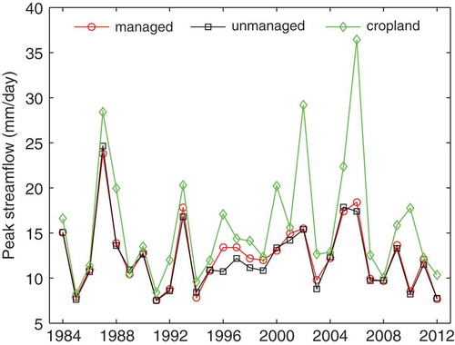
Another useful measure of the impact of management practices on hydrological performance is the annual peak flow. Figure 13 illustrates the simulated peak flow for the period 1984–2012 for the managed forest, unmanaged forest and cropland. Compared to the managed and unmanaged simulations, the cropland scenario shows a dramatic rise in peak runoff, especially during wet years. During drought years the peak runoff is quite similar for all scenarios. However, the model does not account for erosion, which would likely strip away soils and regolith, and so reduce storage and further increase water yield.

Fig. 13 Simulation scenarios for managed forest cutting, unmanaged or no-cutting, and simulated conversion to cropland land use, showing their impact on the annual peak flow for the period 1984–2004.

Figure 14 illustrates the monthly mean runoff (January–December) for all three scenarios, for the period 1984–2012. The managed and unmanaged scenarios are again similar, with the autumn season showing a larger increase in streamflow compared to other seasons (see Appendix Tables A1–A3 for details). Under unmanaged conditions, the greater percentage of older trees consume more water than for the managed case with younger trees. The impact of selective cutting on the water balance is to increase groundwater recharge and baseflow, which tends to alleviate late summer and autumn drought. The cropland scenario (no forest) has consistently larger runoff yield and lower evapotranspiration during all seasons, but especially during wet periods.

Fig. 14 Simulation scenarios for managed forest cutting, unmanaged or no-cutting and simulated conversion to cropland land use showing their impact on the monthly mean streamflow for the period 1984–2004.

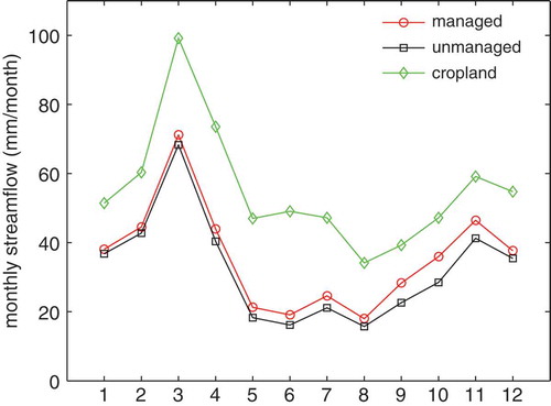
The simulated water budget scenarios demonstrate dramatic differences. For the management case, the net annual runoff is 441.2 mm, while the cropland scenario predicted annual runoff at 671.1 mm. The scenario of unmanaged growth predicted 399.0 mm annual runoff, which shows that the management practices in 1984 and 1994 have increased water yield by 9.5%. Detailed 29-year simulated annual water budgets for each scenario are listed in Tables A1–A3.

4 SUMMARY, CONCLUSIONS AND IMPLICATIONS

It has been suggested that managed plantations can reduce water loss by selective cutting (Vanclay 2009). This modelling study supports that finding and quantifies the explicit impacts of cutting on spatial and temporal water budget dynamics of a Norway spruce watershed in the Czech Republic. The managed scenario of selective cutting has the advantage of reduced water loss and reduction of extreme flooding. Selective cutting forestry operations have been advocated for a wide range of water-related impacts (Van Dijk and Keenan 2007). This simulation study suggests that managed forest in the Lysina catchment, when compared to the unmanaged scenario with no cutting between 1984 and 2012, have similar peak flow responses, lower evaporation and transpiration water losses, and improved runoff status during the late summer and early autumn. When comparing managed and unmanaged forest to the cropland scenario, peak flows are amplified in the latter case. There are definitely other factors that affect hydrological impacts of forest management, such as soil disturbance or compaction, the effect of local atmospheric conditions and plant physiological acclimatization (Van Dijk and Keenan 2007), which are not examined here. Nonetheless, the physics-based hydrologic modelling in this study provides useful insights to the sensitivity of watershed hydrological response to tree cutting history and forest growth.

The study results have demonstrated the utility of physics-based distributed hydrologic modelling, such as PIHM, as a management tool for expanding our understanding of forest hydrological processes and spatially-explicit logging and replanting practice impacts over long periods of time. Compared with previous hydrological studies (Buzek et al. 1995, Krám et al. 1999, Benčoková et al. 2011), the improvements include complete physics-based representation with observed data, localized age-related vegetation dynamics, multi-process integrated modelling of snow accumulation and melting processes, and distributed unsaturated–saturated dynamics. The model’s performance was validated by multi-variables observed at different locations. Simulation of snow accumulation and melt processes was found to be sufficient to capture the spring runoff. The spatial groundwater-table dynamics were obtained using hydrological properties of spatial soil classes. The long-term dynamics of the forest were represented through observed age–LAI relationships. The integrated modelling approach can be useful in assessing the hydrological influence of the spatial configuration of forest management. Scenario simulations suggested the utility of models to future management strategies for assessing sustainable water resources and ecosystem services.

One serious limitation of the study is inadequate ecohydrological observations. Under the framework of CZOs, a real-time ecohydrological monitoring network is under construction at Lysina. The network could provide benchmark hydrological datasets (e.g. meteorological forcing, high-resolution monitoring of spatial groundwater level patterns, stand characteristics and phenology) that will help to simulate the role that hydrolology and hydrogeology play in long-term and short-term runoff (e.g. droughts and floods), as well as long-term climate dynamics and forest management practices. Future research will upgrade to a new level of both data and model, focusing on the spatial representation of groundwater-table dynamics and the ecohydrological impacts of vegetation.

Lysina represents a catchment influenced by intensive forest management, with research priorities that include nutrient leaching, water acidity, metal toxicity and atmospheric deposition (Banwart et al. 2011). This study implemented a distributed integrated hydrologic model, PIHM, with explicit representations of forest management practices. The model combined historical records of land use, existing data and recent field measurements to provide a long-term resolution between available data and mathematical model results. It is interesting to note that, as the forest management-impacted flow pattern changed, the quantity and timing of water yield were observed to influence changes in stream water quality (Hruška and Krám 2003) and soil solution chemistry (Navrátil et al. 2007). This suggests that the model simulation could be applied in future studies on drainage water quality and solute transport. In addition, rapidly changing land use and climate have been found to threaten water resources at many places (Banwart et al. 2011). The projected impacts of global climate change have been estimated with significant impacts likely on both runoff and evapotranspiration at Lysina (Benčoková et al. 2011). The increase in annual evapotranspiration based on model projections was estimated to be 15 to 20%, and annual runoff will decrease by 10 to 30%. The high evapotranspiration changes during the growing season would result in extreme September drought. The scenarios presented here provide insight into the competing impacts of forest management on stream water resources. The hydrological impacts of future climate and forest management can be quantified with integrated hydrologic models and used to project potential approaches to climate change and land use adaptation. Future studies should also address the impact of dynamic phenology induced by climate variability and forest pests. At Lysina, the projected future increase in temperature, and the redistribution of seasonal precipitation, will likely cause decreases in summer and autumn runoff (Benčoková et al. 2011). The model sensitivity of forest management on historical catchment hydrology examined here suggests the utility of models and scenario development for future management strategies, and this will be the subject of future research.

Additional information

Funding

Financial support for this study was provided by the European Commission 7th Framework Programme as a Large Integrating Project (SoilTrEC, www.soiltrec.eu, Grant Agreement no. 244118) and for Jakub Hruška by the Operational Programme of the European Union (CZ.1.05/1.1.00/02.0073).

APPENDIX

Table A1 Water budget of the managed scenario at Lysina.

Year	Interception loss (mm/year)	Transpiration (mm/year)	Evaporation (mm/year)	Groundwater recharge (mm/year)	Runoff (mm/year)	Saturated storage (mm)	Unsaturated storage (mm)
1984	149	185	24	827	570	3234	1017
1985	130	239	27	514	370	3221	1083
1986	141	236	25	634	512	3249	1078
1987	173	197	27	683	664	3280	1165
1988	130	225	25	685	618	3263	1191
1989	130	271	27	606	462	3231	1156
1990	131	258	28	586	437	3226	1140
1991	120	259	29	427	281	3168	1109
1992	146	277	27	655	485	3226	1076
1993	133	276	29	612	451	3232	1096
1994	151	303	31	681	507	3227	1107
1995	152	244	33	662	542	3270	1160
1996	109	190	28	538	444	3269	1176
1997	124	242	29	589	460	3241	1166
1998	143	203	29	634	558	3256	1180
1999	155	233	33	615	501	3262	1226
2000	118	221	24	652	576	3269	1197
2001	136	208	24	610	520	3264	1181
2002	131	202	25	770	723	3289	1260
2003	112	301	26	517	313	3223	1233
2004	113	196	22	618	534	3273	1182
2005	111	213	24	596	522	3271	1227
2006	92	307	29	724	596	3243	1257
2007	91	282	27	671	529	3256	1238
2008	100	271	25	652	514	3238	1224
2009	107	276	26	723	607	3256	1237
2010	83	284	24	576	426	3233	1206
2011	115	317	27	592	406	3221	1191
2012	107	327	27	521	356	3200	1205

Table A2 Water budget of unmanaged scenario at Lysina.

Year	Interception loss (mm/year)	Transpiration (mm/year)	Evaporation (mm/year)	Groundwater recharge (mm/year)	Runoff (mm/year)	Saturated storage (mm)	Unsaturated storage (mm)
1984	163	255	22	812	488	3204	1000
1985	152	345	24	506	292	3125	987
1986	162	340	22	609	398	3182	891
1987	199	286	23	663	548	3237	1015
1988	148	324	21	688	540	3198	1043
1989	149	386	24	594	385	3124	974
1990	148	361	25	553	343	3121	933
1991	135	357	26	350	201	2985	901
1992	165	391	24	682	402	3105	840
1993	149	387	26	610	373	3139	837
1994	167	422	28	650	418	3133	849
1995	209	394	24	648	429	3169	848
1996	150	305	20	504	320	3167	873
1997	162	381	22	525	337	3057	898
1998	190	316	23	576	408	3102	909
1999	199	361	25	607	389	3172	1002
2000	152	343	18	647	466	3182	909
2001	171	323	19	584	405	3170	896
2002	164	309	19	749	579	3235	1048
2003	136	455	21	510	233	3074	1043
2004	137	297	17	594	408	3194	925
2005	147	334	18	574	386	3204	1023
2006	116	478	22	742	457	3143	1074
2007	115	431	21	686	421	3172	1029
2008	121	414	20	655	430	3119	1032
2009	128	421	21	720	461	3166	1049
2010	101	419	20	556	330	3136	985
2011	135	470	23	573	319	3047	970
2012	125	479	23	478	314	3055	967

Table A3 Water budget of cropland scenario at Lysina.

Year	Interception loss (mm/year)	Transpiration (mm/year)	Evaporation (mm/year)	Groundwater recharge (mm/year)	Runoff (mm/year)	Saturated storage (mm)	Unsaturated storage (mm)
1984	32	112	29	902	740	3254	1011
1985	33	144	30	597	542	3286	1060
1986	34	134	29	675	666	3296	1118
1987	36	122	29	758	849	3308	1212
1988	33	130	29	735	777	3305	1230
1989	33	151	30	664	625	3296	1217
1990	35	142	30	642	605	3294	1222
1991	28	154	31	501	434	3266	1196
1992	36	158	30	714	680	3296	1192
1993	34	151	30	682	647	3296	1227
1994	39	158	31	700	663	3298	1246
1995	47	149	31	732	726	3307	1280
1996	31	120	30	595	580	3297	1267
1997	40	151	31	633	592	3285	1256
1998	40	127	30	727	739	3298	1269
1999	42	145	31	682	665	3298	1290
2000	34	139	29	712	722	3301	1270
2001	39	131	29	678	671	3299	1247
2002	35	128	29	828	882	3312	1312
2003	30	174	29	544	470	3284	1286
2004	30	126	28	675	676	3300	1260
2005	24	141	29	661	666	3296	1289
2006	28	159	30	720	783	3291	1302
2007	29	142	29	737	744	3305	1303
2008	33	143	29	672	652	3295	1282
2009	34	153	29	773	792	3298	1290
2010	25	141	29	601	595	3291	1262
2011	33	163	30	660	617	3291	1250
2012	29	167	30	549	509	3287	1261

REFERENCES

- Anderson, E.A., 1973. National Weather Service river forecast system—snow accumulation and ablation model, NOAA Technical Memorandum, NWS HYDRO–17.
- Andréassian, V., 2004. Waters and forests: from historical controversy to scientific debate. Journal of Hydrology, 291 (1–2), 1–27. doi:10.1016/j.jhydrol.2003.12.015.
- Arora, V., 2002. Modeling vegetation as a dynamic component in soil–vegetation–atmosphere transfer schemes and hydrological models. Reviews of Geophysics, 40 (2), 1006. doi:10.1029/2001RG000103.
- Banwart, S., et al., 2011. Soil processes and functions in critical zone observatories: hypotheses and experimental design. Vadose Zone Journal, 10 (3), 974–987. doi:10.2136/vzj2010.0136.
- Banwart, S., et al., 2012. Soil processes and functions across an International Network of Critical Zone Observatories: introduction to experimental methods and initial results. Comptes Rendus Geoscience, 344 (11–12), 758–772. doi:10.1016/j.crte.2012.10.007.
- Benčoková, A., Krám, P., and Hruška, J., 2011. Future climate and changes in flow patterns in Czech headwater catchments. Climate Research, 49 (1), 1–15. doi:10.3354/cr01011.
- Bhatt, G., 2012. A distributed hydrologic modeling system: framework for discovery and management of water resources. Thesis (PhD). Pennsylvania State University.
- Bhatt, G., et al., 2014. A tightly coupled GIS and distributed hydrologic modeling framework. Environmental Modelling & Software, 62, 70–84.
- Bosch, J.M. and Hewlett, J.D., 1982. A review of catchment experiments to determine the effect of vegetation changes on water yield and evapotranspiration. Journal of Hydrology, 55 (1–4), 3–23. doi:10.1016/0022-1694(82)90117-2.
- Brown, A.E., et al., 2005. A review of paired catchment studies for determining changes in water yield resulting from alterations in vegetation. Journal of Hydrology, 310 (1–4), 28–61. doi:10.1016/j.jhydrol.2004.12.010.
- Buzek, F., Hruška, J., and Krám, P., 1995. Three-component model of runoff generation, Lysina catchment, Czech Republic. Water, Air, & Soil Pollution, 79 (1–4), 391–408. doi:10.1007/BF01100449.
- Černý, M., Pařez, J., and Malík, Z., 1996. Growth and yield tables of main tree species of the Czech Republic. Jílové u Prahy: Institute for Forest Ecosystem Research.
- Cohen, S.D. and Hindmarsh, A.C., Dubois, P.F., 1996. CVODE, a stiff/nonstiff ODE solver in C. Computers in Physics, 10 (2), 138–143. doi:10.1063/1.4822377.
- Dooge, J.C.I., 1988. Hydrology in perspective. Hydrological Sciences Journal, 33 (1), 61–85. doi:10.1080/02626668809491223.
- Eisenbies, M.H., et al., 2007. Forest operations, extreme flooding events, and considerations for hydrologic modeling in the Appalachians—A review. Forest Ecology and Management, 242 (2–3), 77–98. doi:10.1016/j.foreco.2007.01.051.
- Ellenberg, H., 1996. Vegetation Mitteleuropas mit den Alpen in ökologischer, dynamischer und historischer Sicht. Stuttgart: Eugen Ulmer Verlag.
- Hock, R., 2003. Temperature index melt modelling in mountain areas. Journal of Hydrology, 282 (1–4), 104–115. doi:10.1016/S0022-1694(03)00257-9.
- Holmberg, M., et al., 2013. Relationship between critical load exceedances and empirical impact indicators at Integrated Monitoring sites across Europe. Ecological Indicators, 24, 256–265. doi:10.1016/j.ecolind.2012.06.013.
- Hornbeck, J.W., et al., 1993. Long-term impacts of forest treatments on water yield: a summary for northeastern USA. Journal of Hydrology, 150 (2–4), 323–344. doi:10.1016/0022-1694(93)90115-P.
- Hruška, J. and Krám, P., 2003. Modelling long-term changes in stream water and soil chemistry in catchments with contrasting vulnerability to acidification (Lysina and Pluhuv Bor, Czech Republic). Hydrology and Earth System Sciences, 7 (4), 525–539. doi:10.5194/hess-7-525-2003.
- Hruška, J., et al., 2009. Increased dissolved organic carbon (DOC) in central European streams is driven by reductions in ionic strength rather than climate change or decreasing acidity. Environmental Science & Technology, 43 (12), 4320–4326. doi:10.1021/es803645w.
- John, D. and Hibbert, A.R., 1961. Increases in water yield after several types of forest cutting. Hydrological Sciences Journal, 6 (3), 5–17.
- Jonas, T., Marty, C., and Magnusson, J., 2009. Estimating the snow water equivalent from snow depth measurements in the Swiss Alps. Journal of Hydrology, 378 (1–2), 161–167. doi:10.1016/j.jhydrol.2009.09.021.
- Kostner, B., Falge, E., and Tenhunen, J.D., 2002. Age-related effects on leaf area/sapwood area relationships, canopy transpiration and carbon gain of Norway spruce stands (Picea abies) in the Fichtelgebirge, Germany. Tree Physiology, 22 (8), 567–574. doi:10.1093/treephys/22.8.567.
- Krám, P., et al., 1995. Biogeochemistry of aluminum in a forest catchment in the Czech Republic impacted by atmospheric inputs of strong acids. Water, Air and Soil Pollution, 85 (3), 1831–1836. doi:10.1007/BF00477246.
- Krám, P., et al., 1997. The biogeochemistry of basic cations in two forest catchments with contrasting lithology in the Czech Republic. Biogeochemistry, 37 (2), 173–202. doi:10.1023/A:1005742418304.
- Krám, P., et al., 1999. Application of the forest–soil–water model (PnET-BGC/CHESS) to the Lysina catchment, Czech Republic. Ecological Modelling, 120 (1), 9–30. doi:10.1016/S0304-3800(99)00064-2.
- Kumar, M., 2009. Toward a hydrologic modeling system, Thesis (PhD). Pennsylvania State University.
- Kumar, M., Bhatt, G., and Duffy, C., 2009. An efficient domain decomposition framework for accurate representation of geodata in distributed hydrologic models. International Journal of Geographical Information Science, 23, 1569–1596. doi:10.1080/13658810802344143.
- Murakami, S., et al., 2000. Variation of evapotranspiration with stand age and climate in a small Japanese forested catchment. Journal of Hydrology, 227 (1–4), 114–127. doi:10.1016/S0022-1694(99)00175-4.
- Nash, J.E. and Sutcliffe, J.V., 1970. River flow forecasting through conceptual models part I—A discussion of principles. Journal of Hydrology, 10 (3), 282–290. doi:10.1016/0022-1694(70)90255-6.
- Navrátil, T., et al., 2007. Acidification and recovery of soil at a heavily impacted forest catchment (Lysina, Czech Republic)—SAFE modeling and field results. Ecological Modelling, 205 (3–4), 464–474. doi:10.1016/j.ecolmodel.2007.03.008.
- Oulehle, F., et al., 2008. Long-term trends in stream nitrate concentrations and losses across watersheds undergoing recovery from acidification in the Czech Republic. Ecosystems, 11 (3), 410–425. doi:10.1007/s10021-008-9130-7.
- Pokorný, R., Tomášková, I., and Havránková, K., 2008. Temporal variation and efficiency of leaf area index in young mountain Norway spruce stand. European Journal of Forest Research, 127 (5), 359–367. doi:10.1007/s10342-008-0212-z.
- Qu, Y. and Duffy, C.J., 2007. A semidiscrete finite volume formulation for multiprocess watershed simulation. Water Resources Research, 43, W08419. doi:10.1029/2006WR005752.
- Robinson, M., et al., 2003. Studies of the impact of forests on peak flows and baseflows: a European perspective. Forest Ecology and Management, 186 (1–3), 85–97. doi:10.1016/S0378-1127(03)00238-X.
- Spinnler, D., Egli, P., and Körner, C., 2002. Four-year growth dynamics of beech-spruce model ecosystems under CO2 enrichment on two different forest soils. Trees-Structure and Function, 16 (6), 423–436. doi:10.1007/s00468-002-0179-1.
- Stednick, J.D., 1996. Monitoring the effects of timber harvest on annual water yield. Journal of Hydrology, 176 (1–4), 79–95. doi:10.1016/0022-1694(95)02780-7.
- Swanson, F.J. and Dyrness, C.T., 1975. Impact of clear-cutting and road construction on soil erosion by landslides in the western Cascade Range, Oregon. Geology (Geological Society of America), 3 (7), 393–396.
- Thanapakpawin, P., et al., 2007. Effects of landuse change on the hydrologic regime of the Mae Chaem river basin, NW Thailand. Journal of Hydrology, 334 (1–2), 215–230. doi:10.1016/j.jhydrol.2006.10.012.
- Vanclay, J.K., 2009. Managing water use from forest plantations. Forest Ecology and Management, 257 (2), 385–389. doi:10.1016/j.foreco.2008.09.003.
- Van Dijk, A.I.J.M. and Keenan, R.J., 2007. Planted forests and water in perspective. Forest Ecology and Management, 251 (1–2), 1–9. doi:10.1016/j.foreco.2007.06.010.
- Wattenbach, M., et al., 2005. A simplified approach to implement forest eco-hydrological properties in regional hydrological modelling. Ecological Modelling, 187 (1), 40–59. doi:10.1016/j.ecolmodel.2005.01.026.
- Wattenbach, M., et al., 2007. Hydrological impact assessment of afforestation and change in tree-species composition—a regional case study for the Federal State of Brandenburg (Germany). Journal of Hydrology, 346 (1–2), 1–17. doi:10.1016/j.jhydrol.2007.08.005.
- Wijesekara, G.N., et al., 2012. Assessing the impact of future land-use changes on hydrological processes in the Elbow River watershed in southern Alberta, Canada. Journal of Hydrology, 412–413, 220–232. doi:10.1016/j.jhydrol.2011.04.018.
- Wösten, J.H.M., Pachepsky, Y.A., and Rawls, W.J., 2001. Pedotransfer functions: bridging the gap between available basic soil data and missing soil hydraulic characteristics. Journal of Hydrology, 251 (3–4), 123–150. doi:10.1016/S0022-1694(01)00464-4.
- Yu, X., et al., 2013. Parameterization for distributed watershed modeling using national data and evolutionary algorithm. Computers & Geosciences, 58, 80–90. doi:10.1016/j.cageo.2013.04.025.