Effects of initial soil water content and saturated hydraulic conductivity variability on small watershed runoff simulation using LISEM

Abstract

Soil water content (θ) and saturated hydraulic conductivity (K_s) vary in space. The objective of this study was to examine the effects of initial soil water content (θ_i) and K_s variability on runoff simulations using the LImburg Soil Erosion Model (LISEM) in a small watershed in the Chinese Loess Plateau, based on model parameters derived from intensive measurements. The results showed that the total discharge (TD) and peak discharge (PD) were underestimated when the variability of θ_i and K_s was partially considered or completely ignored compared with those when the variability was fully considered. Time to peak (TP) was less affected by the spatial variability compared to TD and PD. Except for TP in some cases, significant differences were found in all hydrological variables (TD, PD and TP) between the cases in which spatial variability of θ_i or K_s was fully considered and those in which spatial variability was partially considered or completely ignored. Furthermore, runoff simulations were affected more strongly by K_s variability than by θ_i variability. The degree of spatial variability influences on runoff simulations was related to the rainfall pattern and θ_i. Greater rainfall depth and instantaneous rainfall intensity corresponded to a smaller influence of the spatial variability. Stronger effects of the θ_i variability on runoff simulation were found in wetter soils, while stronger effects of the K_s variability were found in drier soils. For accurate runoff simulation, the θ_i variability can be completely ignored in cases of a 1-h duration storm with a return period greater than 10 years, while K_s variability should be fully considered even in the case of a 1-h duration storm with a return period of 20 years.

Editor D. Koutsoyiannis; Associate editor A. Fiori

Résumé

La teneur en eau du sol (θ) et la conductivité hydraulique à saturation (K_s) varient dans l’espace. L’objectif de cette étude est d’examiner les effets de la variabilité de la teneur initiale en eau du sol (θ_i) et de K_s sur des simulations de ruissellement à l’aide du modèle LImburg d’érosion du sol (LISEM) dans un petit bassin versant du plateau de loess chinois, en se basant sur les paramètres du modèle issus de nombreuses mesures. Les résultats ont montré que le débit total (DT) et le débit de pointe (DP) ont été sous-estimés lorsque la variabilité de θ_i et K_s n'a été que peu ou pas prise en compte, en comparaison avec ceux où la variabilité a été pleinement prise en compte. Le temps jusqu'au pic de crue (TP) a été moins affecté par la variabilité spatiale que DT et DP. Sauf pour TP dans certains cas, des différences significatives ont été trouvées pour toutes les variables hydrologiques (DT, DP et TP) selon que la variabilité spatiale de θ_i ou K_s a été pleinement prise en compte ou bien partiellement ou complètement ignorée. En outre, les simulations de ruissellement ont été affectées plus fortement par la variabilité de K_s que par celle de θ_i. Le degré d'influence de la variabilité spatiale sur les simulations de ruissellement était lié à la distribution de la pluie et à θ_i. Une plus grande hauteur de précipitation et ou intensité instantanée de précipitation correspondaient à de moindres influences de la variabilité spatiale. Les effets les plus importants de la variabilité de θ_i sur la simulation du ruissellement ont été trouvés pour les sols humides, tandis que les effets les plus importants de la variabilité de K_s ont été trouvés pour les sols plus secs. Pour une simulation précise de l'écoulement, la variabilité de θ_i peut être complètement ignorée dans le cas d’une pluie durant une heure et ayant une période de retour supérieure à 10 ans, tandis que la variabilité de K_s devrait être pleinement prise en compte même en cas d'un événement d'une heure ayant une période de retour de 20 ans.

Key words:

• spatial variability
• LISEM
• runoff
• Loess Plateau of China
• soil moisture
• saturated hydraulic conductivity

Mots clefs:

• variabilité spatiale
• LISEM
• ruissellement
• Plateau de loess (Chine)
• humidité du sol
• conductivité hydraulique à saturation

INTRODUCTION

Initial soil water content (θ_i) and saturated hydraulic conductivity (K_s) are important parameters for modelling hydrological processes. A considerable number of studies have witnessed their spatial heterogeneity at different scales (Wilson et al. 1989, Cosh et al. 2004, Taskinen et al. 2008a). Therefore, the possible effects of spatial variability deserve to be taken into account in hydrological modelling (Merz and Plate 1997, Fiori and Russo 2007).

The effects of variability in soil properties on hydrological modelling have been widely reported. Woolhiser et al. (1996) used the method of characteristics to examine the effects of spatial variations in K_s on interactive infiltration and surface runoff on a hillslope, and found that runoff hydrographs were strongly affected by variations in hydraulic conductivity, particularly for small runoff events. Merz and Plate (1997) and Merz and Bárdossy (1998) used SAKE (Simulationsmodell des Abflußverhaltens Kleiner Einzugsgebiete)/FGM (Flussgebietsmodell) and SAKE models to study the effects of spatial variability on the runoff behaviour of a small loess catchment and showed that the spatial patterns and variability could have a dominant control on the rainfall–runoff behaviour. Bronstert and Bárdossy (1999) used a physically-based, distributed hydrological model, called Hillflow to study the effects of θ_i variability on surface runoff generation at the hillslope and small catchment scale. They showed that θ_i variability resulted in an increase in runoff production compared to average values. Herbst and Diekkrüger (2002) used the SWMS_3d model (a computer program for simulating water and solute movement in three-dimensional variably saturated media) to study the effects of frequency distribution and spatial structure of soil hydraulic properties on runoff and concluded that the frequency distribution of hydraulic properties mainly affected the amount of the fast runoff, while the organized spatial variability affected the fast runoff rate. Castillo et al. (2003) observed that the sensitivity of the runoff response to θ_i depended on the predominant runoff mechanisms in three small catchments in semi-arid southeastern Spain, using a simple, physically-based distributed model. In an agricultural catchment in southern Finland, Taskinen et al. (2008b) found that the spatial variability of K_s caused significant variation in overland flow. Based on the Boussinesq equation, Harman and Sivapalan (2009) investigated the effects of lateral variations in hydraulic conductivity on saturated subsurface lateral flow through hillslopes. They indicated that the hillslope-scale response of flow depended on the relative importance of topographic and water table potential gradients in driving flow.

According to the literature review, the spatial distribution of θ_i and hydraulic properties have generally not been intensively measured, although the spatial variability of soil properties has been stressed in hydrological modelling. This may lead to large errors in the spatial distribution of θ_i and hydraulic properties, resulting in major modelling errors. In addition, the relative importance of spatial variability on runoff modelling in different soil water conditions and rainfall were not well defined.

The LImburg Soil Erosion Model (LISEM), which was developed to simulate hydrology and sediment transport, has been widely used. Hessel et al. (2003) discussed the applicability of LISEM and asserted that LISEM could be widely used to simulate watershed soil erosion in the Chinese Loess Plateau. Hessel (2005) explored the effects of grid-cell size and time-step length on LISEM simulation results in the Danangou watershed. At the beginning of LISEM development, De Roo et al. (1996) investigated the sensitivity of LISEM output to changes in input by increasing and decreasing each individual input variable and parameter by 20%. To the best of our knowledge, there are no reports on the response of LISEM output to the spatial variability of θ_i and K_s. In the Chinese Loess Plateau, storm events are usually of short duration, with soil erosion in this area mainly caused by short storms of 1-h duration (Zhang 1983). Therefore, a study of hydrological modelling response to spatial variability of soil properties is very important for flooding and soil erosion forecasting in this area. Furthermore, it will also enrich our understanding of the influences of spatial variability on hydrological modelling under different environmental backgrounds.

The objective was to explore the influence of the spatial variability of θ_i and K_s on the simulated values of three important hydrological variables: total discharge (TD), peak discharge (PD), and time to peak (TP). Based on model parameters derived from intensive measurements, runoff was simulated by the hydrological module of LISEM in a small watershed in the Chinese Loess Plateau under various rainfall and initial soil water conditions.

MATERIALS AND METHODS

The LISEM model

The LISEM model has two parts: a water part and an erosion part. Only the water part, which considers such basic processes as rainfall, interception, surface storage, infiltration, vertical movement of water in the soil, overland flow and channel flow, was used in this study. Detailed information on LISEM can be found in De Roo et al. (1996), Jetten and De Roo (2001) and Hessel (2005). Several infiltration models are incorporated in this model: in this study, the Green-Ampt equation for one layer was used because of the relatively uniform soil profile in the watershed (Li et al. 1976).

Study area

A small watershed called LaoYeManQu (LYMQ) with an area of 0.2 km² was selected inside the larger Liudaogou watershed (110º21ʹ–110º23ʹE; 38º46ʹ–38º51ʹN) in Shenmu County, Shaanxi Province, China (Fig. 1). This area has cold semi-arid climate, with a mean annual temperature of 8.4°C, and a mean annual precipitation of 437 mm year^-1, half of which is received between June and September (Tang et al. 1993). Storm events are usually of short duration, and cause severe soil erosion. The Chinese Loess Plateau is characterized by its landscape of deep gullies and undulating slopes. The LYMQ watershed ranges in elevation from 1056–1130 m a.s.l., with soils dominated by Inceptisols with a sandy loam texture (Soil Survey Staff 2010). The dominant vegetation species are bunge needlegrass (Stipa bungeana Trin.) and korshinsk peashrub (Caragana Korshinskii kom.). Nine different types of land use can be identified, according to the dominant vegetation, its coverage and soil type.

Fig. 1 Land-use distribution and sampling locations in the LYMQ watershed.

Model parameters

Rainfall

Rainfall depths recorded for 15 rainfall events from June to September 2007 at 21 random locations in the LYMQ watershed, showed coefficients of variation of generally less than 10%. The semi-variograms of rainfall depth indicated that its variability was purely random (not shown). Therefore, the spatial variability of rainfall was neglected. Based on the hourly rainfall record in this area, 1-h duration storm events with rainfall depths of 25, 33 and 44 mm, corresponding to return periods of 5, 10 and 20 years, respectively, were used for simulation (Zhang 1983). Taking into consideration the slope angle in this watershed, the effective rainfall depths on the land surface were 19.1, 25.2 and 33.6 mm, respectively. To determine whether instantaneous rainfall intensity influences the response of runoff generation to spatial variability of θ_i and K_s, three temporal patterns of rainfall distribution, with 10, 50 and 90% probability curves, were simulated for each rainfall depth (Pani and Haragan 1981). They represent 22.5, 56.0 and 82.5%, respectively, of the total rainfall being received in the first half hour of rainfall events. The maximum instantaneous rainfall intensity was highest for a storm probability level of 10% and lowest for the 50% level.

Input maps

The model parameters and data collection methods are summarized in Table 1. Maps used as spatial input are shown in Fig. 2. As the spatial variability of θ_i and K_s was the main consideration, further detailed information on deriving θ_i and K_s maps is presented below.

Table 1 Model parameters and data collection.

Parameter	Explanation	Data collection method
Rainfall		Three rainfall depths and three temporal patterns of rainfall were used (refer to text for details)
Catchment maps
AREA	Catchment boundaries	Derived by the PCRaster using DEM (Hu et al. 2010)
GRAD	Slope gradient	Derived by the PCRaster using DEM (Hu et al. 2010)
LDD	Local drainage direction	Derived by the PCRaster using DEM (Hu et al. 2010)
OUTLET	Location of outlet	Set to 1 at the watershed outlet and 0 elsewhere
ID	Area covered by raingauges	Set to 1 for the whole watershed without considering spatial variability of rainfall
Vegetation maps
LAI	Leaf area index	Estimated by counting the leaf number and measuring mean leaf area; three replicates were made and averaged for each land use
PER	Fraction of soil covered by vegetation	Estimated visually; three replicates were made and averaged for each land use
CH	Vegetation height	Measured by a ruler; three replicates were made and averaged for each land use
Soil surface maps
RR	Random roughness—standard deviation of the surface micro-relief, usually measured by pin method (Cremers et al. 1996)	Surface roughness (TA) was measured by chain method (Saleh 1993) at 169 points (shown in Fig. 1) and converted to RR by considering (Linden et al. 1988, Morgan et al. 1998): RETmax = 0.112RR + 0.031RR^2 – 0.012RR·S = exp[−6.66 + 0.27(TA)] where RETmax is the maximum depressional storage and S is slope (%). Ordinary kriging was used to interpolate for the RR map
N	Manning’s n	Derived from that calibrated in the Danangou watershed in the same area (Hessel et al. 2003)
COMPFRC	Fraction of soil surface compacted by wheel track	Set to 0
STONEFR	Fraction of soil surface covered by stones	Set to 0
CRUSTFRC	Fraction of soil surface covered with crust	Estimated visually; three replicates were made and averaged for each land use
ROADWIDT	Width of impermeable roads	Set to 0
GRASSWIDT	Width of grass strips	Set to 0
Infiltration related maps
θi	Initial soil water content	Intensive measurements by neutron probe (refer to text for details)
Ks	Saturated hydraulic conductivity	Intensive measurements by constant-head method (Klute and Dirksen 1986) (refer to text for details)
θs	Saturated volumetric soil water content (soil porosity)	Soil bulk density of 0–0.05 m was measured by gravimetric method at 169 points (Fig. 1). Soil porosity was calculated from soil bulk density assuming a soil density of 2.65 g cm^-3. Ordinary kriging was used to interpolate the θs map
PSI1	Soil water tension at the wetting front (the reciprocal of pore-size distribution parameter, α)	α was measured by a disc infiltrometer at all points shown in Fig. 1, except for those in the gully (Hu et al. 2008, 2009). Ordinary kriging was used to interpolate the PS1 map
SOILDEP1	Soil depth	Soil depth ranges from 50 to 80 m, SOILDEP1 was set to 1000 mm, which is deep enough for the rainfall–runoff simulation

Fig. 2 Model parameters in the watershed required for runoff simulation using LISEM. All parameters are explained in Table 1.

Assuming that θ_i and K_s are uniform throughout the soil profile, measurements of θ_i for 0–0.4 m and K_s for 0–0.05 m at 169 sampling locations were used (Fig. 1). The volumetric soil water content at a depth of 0–0.4 m, was measured by a neutron probe on three different dates (7 June, 4 May and 21 June) in 2008 under various soil water conditions. As a simplification, soil water contents on these three days were divided into three classes: low (θ_L), moderate (θ_M), and high (θ_H), respectively (details of the θ_i are provided in the Results and Discussion Section). An undisturbed soil core (0.005 m height, 0.002 m² cross-sectional area) was taken from the surface 0–0.05 m of soil at each of the 169 sampling locations (Fig. 1), and subsequently transported to a laboratory and saturated. The K_s value of each core was measured by the constant-head method (Klute and Dirksen 1986, Hu et al. 2013). The calibrated LISEM model in Danangou watershed in the same area was used with K_s multiplied by an adjustment factor of 0.3 (Stolte et al. 2003). Statistical analysis of θ_i and K_s was performed using the Statistical Program for Social Sciences (SPSS) 11.0 (SPSS Inc., 2001) and gstat (Pebesma and Wesseling 1998).

To determine the effects of θ_i and K_s variability on runoff simulations, three spatial patterns were considered for θ_i and K_s. For the first pattern, the spatial variability was fully considered and their distributions were constructed as the mean values of 100 Gaussian conditional simulations (FC). Gaussian conditional simulation does not aim to reduce local error variance as kriging does, but focuses on the reproduction of statistics such as the semi-variogram model (Goovaerts 1999). The method is conditional because it honours the location and value of known data points and simulates Gaussian distributed values elsewhere (Haneberg 2006). The model assumes that each variable of interest is normally distributed. According to the Q-Q plots of θ_i and K_s (not shown), θ_i values on the three measurement dates conform to a normal distribution, whereas K_s conforms to a lognormal distribution. Therefore, a log-transformation was made to K_s prior to Gaussian conditional simulation. The original K_s value was obtained by taking 10 to the power of averaged log₁₀K_s. A normal score back-transformation was applied to each set of simulation results to produce a simulated variable distribution with the same statistical distribution as the measured values. Each new simulated value was calculated using the nearest 20 known or previously simulated values. The gstat software (Pebesma and Wesseling 1998) was used to run Gaussian conditional simulation. For the second pattern, the spatial variability was partially considered: the mean value of each land use was assigned to the corresponding land-use class (PC); and for the last pattern, the spatial variability was not considered and the mean value of all sampling locations was assigned to the entire watershed (NC).

Runoff simulation and analysis

For each θ_i and K_s, a total of 81 simulations (3 rainfall depths × 3 temporal patterns of rainfall × 3 initial soil water contents × 3 spatial patterns of θ_i or K_s) were run with LISEM (Jetten 2002). The θ_i variability was fully considered when the aim was to study the effects of K_s variability on runoff simulation. Similarly, the K_s variability was fully considered when the effect of θ_i variability on runoff simulation was studied. For each run, a hydrograph (i.e. runoff rate vs time) was simulated, and three hydrological variables, TD, PD and TP, were obtained from the hydrograph.

To test the significance of differences in the simulated values of TD, PD and TP between the FC and PC (or NC) patterns, in terms of θ_i or K_s, paired sample t-tests were conducted using SPSS 11.0. In each hypothesis testing, pairwise values of hydrological variables were generated under the same conditions, i.e. the same rainfall depth, temporal pattern of rainfall distribution, and initial soil water content. Similarly, paired sample t-tests were also conducted to determine the significance of differences in the simulated values of hydrological variables between FC and PC (or NC) patterns under each specific condition

In order to quantitatively determine the overall effects of spatial variability on runoff simulation, the relative difference (RD%) in the simulated values of TD, PD and TP between the PC (or NC) and FC patterns was calculated (Merz and Plate 1997):

(1)

where X refers to the simulated value of a hydrological variable in the PC (or NC) pattern, and the subscript ‘FC’ refers to the FC pattern for θ_i or K_s. Negative RD% means hydrological variables in the PC (or NC) pattern were underestimated compared with the FC pattern, and vice versa.

RESULTS AND DISCUSSION

Spatial variability of θ_i and K_s

Based on the field campaigns, the mean θ_L, θ_M and θ_H were 0.079 (7 June), 0.114 (4 May) and 0.165 (21 June), respectively. The corresponding standard deviations were 0.047, 0.057 and 0.062, respectively (Table 2). This suggests that θ_i variation was greater in wetter conditions (De Lannoy et al. 2006, Hu et al. 2011). However, a steady increase in θ_i variation from a dry to a saturated state was not observed, as indicated by the reduced standard deviations of saturated soil water content (θ_s) (Table 2). This result is in agreement with the convex relationship observed between standard deviations and mean θ in wet areas (Romshoo 2004, Penna et al. 2009). As others have previously found (Penna et al. 2009, Hu et al. 2011), the coefficient of variation decreased with increasing θ_i. The mean log₁₀K_s (in log₁₀(mm h^-1)) was 1.5, with a standard deviation of 0.476. Statistical analysis with the original K_s showed that the mean K_s value was 60.0 mm h^-1, with a standard deviation of 76.8 mm h^-1 and coefficient of variation of 1.28. This indicates that the spatial variability of K_s was much stronger than that of θ_i.

Table 2 Summary of statistics for θ_i, θ_s and log₁₀K_s of the study site.

Variables	Classical statistics						Geostatistics
	Min.	Max.	Mean	Std. deviation	CV^†	Skewness	Kurtosis	Nugget	Structured variance	Sill	Nugget/Sill	Range (m)
θL [V V^-1]	0.014	0.270	0.079	0.047	0.588	1.074	1.687	0.0011	0.0014	0.0025	0.43	130.4
θM [V V^-1]	0.029	0.334	0.114	0.057	0.503	0.784	0.920	0.0018	0.0021	0.0038	0.46	138.1
θH [V V^-1]	0.043	0.335	0.165	0.062	0.373	−0.154	−0.283	0.0014	0.0032	0.0046	0.30	149.6
θs [V V^-1]	0.377	0.633	0.465	0.038	0.081	0.162	1.400	0.0006	0.0011	0.0016	0.34	185.9
log10Ks (Ks in mm h^-1)	0.260	2.599	1.500	0.476	0.317	0.455	−0.373	0.0608	0.5241	0.5849	0.40	191.7

^†CV: coefficient of variation.

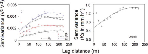
Both θ_i and K_s presented a well-organized spatial pattern as analysed by variograms (Fig. 3). A spherical variogram model (Pebesma and Wesseling 1998) gave a good fit to the experimental semi-variances, with a significance level of P < 0.01 (Table 2). Both structured variance (sill-nugget) (Atkinson and Lewis 2000, Hu et al. 2011) and sill increased from θ_L to θ_H. This implies that increased θ_i variability was mainly contributed by the structure variability. The ratio of nugget to sill was greater for θ_H than for θ_L and θ_M, and the range of correlation increased with increasing θ_i. This implies that θ_i presented stronger spatial dependency over a longer distance in wetter conditions. Both nugget and sill of θ_s were less than those of unsaturated soil water contents (Table 2), verifying again the decreased variability at saturated conditions. Furthermore, θ_s presented a longer range of correlation than unsaturated soil water contents. Saturated hydraulic conductivity showed moderate spatial dependency, with a ratio of nugget to sill of 0.40. The range of correlation was 191.7 m, greater than that of θ_s. One can refer to Hu et al. (2013) for detailed information on K_s variability in this watershed.

Fig. 3 Experimental (symbols) and theoretical (lines) semi-variance of initial soil water content, saturated soil water content (θ_s) and log-transformed saturated hydraulic conductivity (log₁₀K_s) in the small watershed.

Gaussian conditional simulations of θ_i and K_s were based on the spherical variogram model developed in Fig. 3 and Table 2. Figure 4 shows the first three realizations of Gaussian conditional simulation for θ_i (May 4) and log₁₀K_s. All three realizations show θ_i or log₁₀K_s patterns that are similar on a gross scale but differ in detail due to the variation. When realizations were averaged, the simulated distribution would approximate the real condition in a more stable way. The performance of Gaussian conditional simulation has been deemed to be robust for soil properties (especially for hydraulic properties) interpolation (Goovaerts 1999). The number of simulations (100) in this study was much larger than in other studies (e.g. Holmes et al. 2000, Haneberg 2006). With an increasing number of simulations, the mean simulated values approached constant values. It was found that 10 simulations (for θ_i) and 60 simulations (for K_s) generated mean simulated values very similar to those from 100 simulations, with spatial mean absolute values of RD% less than 5%. Therefore, 100 simulations were adequate to obtain a reliable distribution of θ_i and K_s. Compared with individual realizations, the mean of 100 simulations was more continuous in space, but it was also similar to each realization on a gross scale (Fig. 5). As shown in Fig. 5, the FC pattern is distinctly different from the PC and NC patterns in terms of θ_i and K_s.

Fig. 4 Three of the 100 realizations generated for (a) θ_M and (b) log₁₀K_s in the small watershed using Gaussian conditional simulations.

Fig. 5 Various spatial patterns of (a) θ_M and (b) K_s in the small watershed.

Effects of spatial variability of θ_i on runoff simulation

Hydrographs simulated with different θ_i patterns under all cases are shown in Fig. 6. Table 3 lists all simulated values of hydrological variables in the FC pattern for both θ_i and K_s. TD and PD increased with increasing rainfall depth and θ_i, as expected. For the same rainfall depth, the simulated TD and PD ranked as 10% > 90% > 50% in terms of rainfall pattern. This indicates that, for the same amount of rainfall, higher instantaneous rainfall intensity generated more runoff. In contrast, simulated TP decreased with increasing θ_i and rainfall depth, indicating an earlier arrival of peak discharge. For the same rainfall depth, the simulated TP ranked as 10% > 50% > 90% in terms of rainfall pattern, which agrees with the sequence of rainfall depths in the second half hour.

Table 3 Simulated values of hydrological variables when spatial variability of θ_i and K_s were fully considered.

Rainfall		Total discharge (mm)			Peak discharge (L s^-1)			Time to peak (min)
Rainfall depth	Temporal pattern	θL	θM	θH	θL	θM	θH	θL	θM	θH
25 mm	10%	0.50	0.67	1.04	98.3	133.4	212.9	61.0	60.3	59.3
	50%	0.20	0.32	0.58	40.3	57.6	106.4	53.0	53.0	52.5
	90%	0.45	0.62	0.99	88.3	120.4	200.4	42.5	42.0	41.0
33 mm	10%	2.51	2.91	3.62	561.8	648.8	806.0	56.8	56.5	56.0
	50%	1.71	2.07	2.75	331.6	394.0	521.8	49.0	48.8	48.3
	90%	2.45	2.85	3.56	527.8	614.5	769.2	38.8	38.3	37.5
44 mm	10%	7.01	7.64	8.68	1573.5	1692.8	1887.1	54.3	54.0	53.5
	50%	5.78	6.40	7.46	1105.8	1203.9	1363.6	45.5	45.3	44.5
	90%	6.90	7.52	8.55	1515.0	1633.8	1838.0	35.3	35.0	34.5

Fig. 6 Hydrographs simulated with different spatial patterns of initial soil water content (θ_i) under different rainfall events and initial soil water contents.

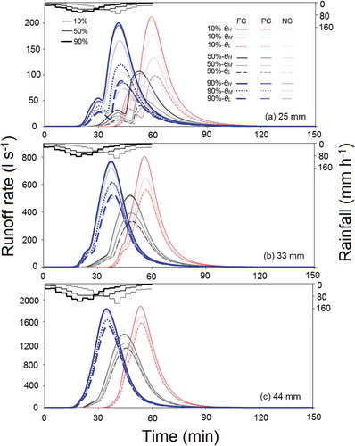
For the PC and NC patterns, the simulated values of hydrological variables presented similar trends to those observed in the FC pattern, although they differed in θ_i patterns (Fig. 6). The hydrographs simulated by the NC and PC patterns were lower than those simulated by the FC pattern, with the hydrograph simulated by the NC pattern the lowest. The paired samples t-test indicates that the simulated values of TD, PD and TP were significantly (P < 0.001 or P < 0.05) different between FC and PC (or NC) patterns in terms of θ_i when all simulations were considered (Table 4).

Table 4 Paired samples t-test results for the differences in simulated values of hydrological variables between different spatial patterns in terms of θ_i and K_s.

Case*	Variable	Pair^†	Paired differences in terms of θi				Paired differences in terms of Ks
			Mean	Std. deviation	t value	Sig.	Mean	Std. deviation	t value	Sig.
All	TD (mm)	FC-PC	5.3	1.9	14.2	<0.001	290.1	152.8	9.9	<0.001
		FC-NC	39.7	19.3	10.7	<0.001	746.9	546.4	7.1	<0.001
	PD (L s^-1)	FC-PC	5.9	2.9	10.4	<0.001	222.0	115.1	10.0	<0.001
		FC-NC	29.8	12.3	12.6	<0.001	626.7	459.4	7.1	0.017
	TP (min)	FC-PC	−0.1	0.3	−2.6	0.016	−2.3	4.7	−2.5	<0.001
		FC-NC	−0.4	0.4	−4.6	<0.001	11.2	19.0	3.1	<0.001
25 mm	TD (mm)	FC-PC	4.7	2.3	6.2	<0.001	110.9	36.7	9.1	<0.001
		FC-NC	23.5	11.5	6.1	<0.001	146.1	68.6	6.4	<0.001
	PD (L s^-1)	FC-PC	3.2	1.5	6.6	<0.001	88.8	32.0	8.3	<0.001
		FC-NC	20.6	8.8	7.0	<0.001	117.6	58.2	6.1	<0.001
	TP (min)	FC-PC	−0.3	0.4	−2.5	0.035	−4.3	7.8	−1.7	0.136
		FC-NC	−0.9	0.3	−9.1	<0.001	32.4	17.3	5.6	0.001
33 mm	TD (mm)	FC-PC	5.5	1.6	10.3	<0.001	286.2	20.9	41.0	<0.001
		FC-NC	42.8	16.8	7.7	<0.001	664.0	149.9	13.3	<0.001
	PD (L s^-1)	FC-PC	6.4	1.5	13.3	<0.001	222.5	28.1	23.7	<0.001
		FC-NC	34.7	13.9	7.5	<0.001	571.9	152.7	11.2	<0.001
	TP (min)	FC-PC	−0.1	0.1	−1.5	0.169	−1.8	1.0	−5.2	0.001
		FC-NC	−0.2	0.1	−4.0	0.004	4.8	8.9	1.6	0.141
44 mm	TD (mm)	FC-PC	5.9	2.0	8.9	<0.001	473.2	17.4	81.8	<0.001
		FC-NC	52.8	17.1	9.2	<0.001	1430.6	56.9	75.5	<0.001
	PD (L s^-1)	FC-PC	8.0	3.3	7.3	<0.001	354.8	37.7	28.2	<0.001
		FC-NC	34.0	8.6	11.9	<0.001	1190.6	81.0	44.1	<0.001
	TP (min)	FC-PC	0.0	0.2	−0.6	0.594	−0.7	0.1	−18.9	<0.001
		FC-NC	−0.1	0.1	−1.5	0.169	−3.6	1.5	−6.9	<0.001
10%	TD (mm)	FC-PC	5.4	2.1	7.8	<0.001	301.2	155.9	5.8	<0.001
		FC-NC	39.6	18.7	6.4	<0.001	778.4	544.2	4.3	0.003
	PD (L s^-1)	FC-PC	6.6	2.9	6.7	<0.001	244.0	120.0	6.1	<0.001
		FC-NC	31.8	12.2	7.8	<0.001	687.0	481.3	4.3	0.003
	TP (min)	FC-PC	−0.1	0.1	−2.5	0.035	−2.0	1.8	−3.3	0.011
		FC-NC	−0.4	0.3	−3.2	0.012	5.3	10.8	1.5	0.177
50%	TD (mm)	FC-PC	5.5	1.8	9.3	<0.001	274.0	169.5	4.8	0.001
		FC-NC	40.0	22.6	5.3	0.001	689.5	603.5	3.4	0.009
	PD (L s^-1)	FC-PC	4.3	1.7	7.8	<0.001	184.5	107.1	5.2	0.001
		FC-NC	25.6	11.4	6.7	<0.001	523.7	451.8	3.5	0.008
	TP (min)	FC-PC	−0.2	0.4	−1.5	0.169	−2.1	7.7	−0.8	0.442
		FC-NC	−0.3	0.4	−2.3	0.050	21.2	25.0	2.5	0.034
90%	TD (mm)	FC-PC	5.1	2.2	7.0	<0.001	295.2	149.8	5.9	<0.001
		FC-NC	39.4	18.6	6.4	<0.001	772.8	551.5	4.2	0.003
	PD (L s^-1)	FC-PC	6.7	3.5	5.7	<0.001	237.5	121.6	5.9	<0.001
		FC-NC	31.9	13.4	7.1	<0.001	669.4	481.8	4.2	0.003
	TP (min)	FC-PC	−0.1	0.2	−1.4	0.195	−2.7	2.6	−3.1	0.015
		FC-NC	−0.4	0.5	−2.4	0.043	7.1	16.2	1.3	0.225
θL	TD (mm)	FC-PC	3.2	0.9	10.7	<0.001	267.8	163.0	4.9	0.001
		FC-NC	24.6	9.8	7.5	<0.001	671.5	566.0	3.6	0.007
	PD (L s^-1)	FC-PC	5.8	2.5	7.0	<0.001	208.1	126.1	5.0	0.001
		FC-NC	20.9	6.3	9.9	<0.001	579.1	496.4	3.5	0.008
	TP (min)	FC-PC	−0.3	0.4	−2.1	0.073	−1.0	6.2	−0.5	0.649
		FC-NC	−0.4	0.4	−2.7	0.026	15.3	20.7	2.2	0.058
θM	TD (mm)	FC-PC	5.6	1.0	16.5	<0.001	287.6	159.9	5.4	0.001
		FC-NC	36.0	13.4	8.1	<0.001	732.1	568.0	3.9	0.005
	PD (L s^-1)	FC-PC	4.6	3.1	4.4	0.002	220.2	121.6	5.4	0.001
		FC-NC	26.2	8.5	9.3	<0.001	618.9	485.9	3.8	0.005
	TP (min)	FC-PC	−0.1	0.1	−2.0	0.081	−3.5	4.9	−2.2	0.062
		FC-NC	−0.4	0.5	−2.4	0.044	9.8	18.9	1.6	0.158
θH	TD (mm)	FC-PC	7.2	1.2	17.5	<0.001	315.0	150.1	6.3	<0.001
		FC-NC	58.4	16.3	10.7	<0.001	837.1	558.0	4.5	0.002
	PD (L s^-1)	FC-PC	7.3	2.9	7.6	<0.001	237.8	109.0	6.5	<0.001
		FC-NC	42.2	9.9	12.8	<0.001	682.1	444.4	4.6	0.002
	TP (min)	FC-PC	−0.1	0.2	−0.8	0.447	−2.3	2.2	−3.2	0.012
		FC-NC	−0.4	0.4	−2.6	0.032	8.6	19.1	1.4	0.214

*All: all simulations were included in the paired sample t-tests (df = 26); 25 m, 10% and θ_L: simulations with rainfall depth of 25 mm, rainfall pattern of 10%, and low initial soil water content were included, respectively, in the paired sample t-tests (df = 8), others can be understood by analogy.

^† Significant (P < 0.001 or P < 0.05) differences in simulated values between the PC and NC patterns were also observed, with the exception of TP in some cases. Results of pairwise comparison between PC and NC are not listed, because the focus was to compare the simulated values between PC (or NC) and FC patterns.

Table 5 lists the RD% of simulated values of hydrological variables under different θ_i and rainfall events. All RD% values of TD and PD were negative, and the absolute values of RD% in the NC pattern were greater than those in the PC pattern. This implies that TD and PD were underestimated in all cases; more underestimations were obtained when spatial variations were not considered. The underestimations of TD and PD in all cases could be the reason why the differences between the FC and PC (or NC) patterns were statistically significant. Infiltration excess reproduced by the LISEM model is the main runoff production mechanism (Yang et al. 2012), although saturation excess is also likely to exist in this area. The coarse texture (silt loam to sand) and high K_s of the soils do not favour runoff generation. This was why only one small runoff event took place between 2007 and 2008. Nevertheless, the areas with relatively high θ_i tend to generate runoff under a certain storm type. When θ_i was averaged over an area, the contributing areas for runoff generation were smaller due to the increased infiltrability induced by the decrease of θ_i. This resulted in underestimation of TD and PD.

Table 5 Relative difference (RD%) of simulated values of hydrological variables for NC and PC patterns of θ_i.

Rainfall		θL-NC	θL-PC	θM-NC	θM-PC	θH-NC	θH-PC
Rainfall depth	Temporal pattern
Total discharge
	10%	−11.3	−1.6	−12.8	−2.9	−15.7	−2.8
25 mm	50%	−22.8	−6.3	−22.5	−5.8	−23.4	−4.8
	90%	−12.3	−1.5	−13.5	−2.8	−16.7	−3.3
	10%	−4.4	−0.6	−5.5	−0.8	−7.1	−0.7
33 mm	50%	−5.7	−1.0	−7.2	−1.5	−9.6	−1.2
	90%	−4.5	−0.6	−5.6	−0.8	−7.3	−0.6
	10%	−2.0	−0.2	−2.6	−0.4	−3.3	−0.4
44 mm	50%	−2.7	−0.2	−3.4	−0.4	−4.4	−0.3
	90%	−2.0	−0.2	−2.6	−0.3	−3.3	−0.4
Peak discharge
	10%	−15.3	−2.4	−13.2	−1.7	−16.2	−2.4
25 mm	50%	−29.1	−11.1	−25.0	−4.1	−24.5	−3.6
	90%	−17.0	−3.9	−13.6	−0.4	−17.1	−2.4
	10%	−4.9	−1.3	−5.3	−1.1	−6.9	−1.0
33 mm	50%	−4.7	−1.2	−5.6	−1.0	−8.6	−1.3
	90%	−4.7	−1.4	−5.7	−1.1	−6.9	−0.9
	10%	−1.7	−0.6	−2.0	−0.4	−2.1	−0.6
44 mm	50%	−2.2	−0.5	−2.5	−0.1	−2.9	−0.5
	90%	−1.7	−0.6	−1.9	−0.6	−2.8	−0.7
Time to peak
	10%	1.6	0.4	1.2	0.0	0.8	0.0
25 mm	50%	0.9	2.4	1.4	0.5	2.4	1.0
	90%	2.4	1.2	3.0	0.6	1.8	0.0
	10%	0.4	0.4	0.4	0.4	0.4	0.0
33 mm	50%	0.5	0.0	0.0	0.0	0.0	0.0
	90%	0.0	0.0	0.7	0.0	0.7	0.0
	10%	0.0	0.0	0.0	0.0	0.5	0.5
44 mm	50%	0.5	0.5	0.0	0.0	0.0	−0.6
	90%	0.0	0.0	0.0	0.0	0.0	0.0

In general, the absolute value of RD% was less than 10% when rainfall depth exceeded 25 mm in the PC pattern and 33 mm in the NC pattern. This indicates that fully considering θ_i variability may not always be necessary for runoff simulation. In our case, considering the θ_i variability based on land-use type only is sufficient to obtain satisfactory simulation results for rainfall with a return period greater than 5 years. For rainfall with a return period greater than 10 years, θ_i variability is not important. In this situation, accurate estimation of mean soil water content, rather than θ_i variability, should be emphasized for runoff simulation.

Although the differences in TP between the FC and PC (or NC) patterns were statistically significant, the RD% values for TP were very small. From the physical point of view, therefore, TP may be hardly affected, whether partially considering or completely ignoring the spatial variability of θ_i. This means that the spatial variability of θ_i can be ignored only if the aim is to forecast the time of peak flood.

The paired samples t-test result indicates that the hydrological variables (with the exception of TP in some cases) were significantly (P < 0.001 or P < 0.05) different between the FC and PC (or NC) patterns in terms of θ_i (Table 4). However, the influences of θ_i variability on simulated TD and PD varied with rainfall event and θ_i, as quantified by RD% (Table 5). The absolute values of RD% for TD and PD decreased with the increase of rainfall depth, indicating a decrease of simulation difference for a larger storm. The absolute value of RD% for TD and PD in general ranked as 50% > 90% > 10% in terms of rainfall pattern. This result indicates that simulation difference decreased with the increase of instantaneous rainfall intensity. The interaction between rainfall and θ_i variability on runoff simulation may be related to the infiltration excess mechanism of runoff generation. When rainfall intensity increases, runoff can be found in larger areas, and the response of soil to rainfall is more homogeneous. This result is in agreement with Castillo et al. (2003), who observed no effects of θ_i variability on runoff under a rainfall intensity of 50 mm h^-1.

With the increase of θ_i, the absolute values of RD% for TD and PD showed an increasing trend. This implies that in wetter conditions θ_i variability has a greater influence on runoff. The greater variability of θ_i in wetter conditions should mainly contribute to this increased influence (Table 2 and Fig. 3). Since the spatial variability of soil water content is positively correlated with the mean soil water content in arid and semi-arid areas (Hu et al. 2011), it may be inferred that more attention should be paid to θ_i variability in wetter conditions for runoff simulation. However, the influence of θ_i variability on runoff simulation may decrease beyond a certain mean soil water content considering the reduced θ variability at the saturated point (Table 2 and Fig. 3). Very high soil water content is difficult to develop in arid and semi-arid areas, but this is usual in humid areas, where spatial variability of θ is observed to be negatively correlated with mean θ (Grayson et al. 1997). Therefore, the influence of θ_i variability on runoff simulation is likely to be less under wetter conditions in humid areas, although it may need further verification.

Effects of spatial variability of K_s on runoff simulation

Similar to θ_i, the simulated hydrographs for K_s present similar trends with different rainfall events and initial soil water contents among the FC, PC and NC patterns (Fig. 7). However, the hydrographs simulated by the NC and PC patterns were much lower than those simulated by the FC pattern. The hydrograph simulated by the NC pattern was the lowest, with almost no runoff observed for rainfall depths of 25 and 33 mm. The paired samples t-test result indicates that the simulated mean values of the hydrological variables (TD, PD and TP) were significantly (P < 0.001 or P < 0.05) different between the FC and PC (or NC) patterns in terms of K_s when all simulations were considered (Table 4).

Fig. 7 Hydrographs simulated with different spatial patterns of saturated hydraulic conductivity (K_s) under different rainfall events and initial soil water contents.

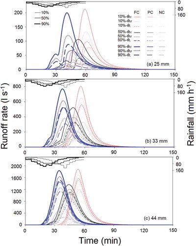
Table 6 lists the RD% of simulated runoff under different θ_i and rainfall events. For all the θ_i conditions and rainfall events, very low runoff occurred for the NC pattern, hence the RD% value of TD and PD was great, even approaching −100% for rainfall depths of 25 and 33 mm. The K_s spatial variability cannot be ignored for runoff simulation in this watershed. For the PC pattern, the simulated runoff was also largely underestimated, with RD% of PD ranging from −20.2 to −100%. In this watershed, K_s presented a well-organized and highly spatial variability (Table 2 and Fig. 3). Runoff tends to occur in areas with relatively low K_s values. When K_s variability was partially or completely ignored, K_s values in areas with low infiltration were artificially increased. Therefore, very limited areas contributed to the watershed-scale runoff, resulting in much less or even no runoff. As for TP, the absolute value of RD% was much less than that of TD and PD, whereas it was much larger when θ_i variability was not fully considered.

Table 6 Relative difference (RD%) of simulated values of hydrological variables for NC and PC patterns of K_s.

Rainfall		θL-NC	θL-PC	θM-NC	θM-PC	θH-NC	θH-PC
Rainfall depth	Temporal pattern
Total discharge
	10%	−100.0	−82.6	−100.0	−74.7	−100.0	−63.1
25 mm	50%	−100.0	−100.0	−100.0	−95.2	−100.0	−81.3
	90%	−100.0	−87.0	−100.0	−78.5	−100.0	−66.2
	10%	−99.8	−44.3	−99.5	−40.5	−98.2	−34.9
33 mm	50%	−100.0	−58.8	−100.0	−53.5	−100.0	−45.3
	90%	−100.0	−46.1	−99.9	−41.8	−99.6	−35.3
	10%	−80.0	−27.1	−75.5	−25.8	−69.0	−23.6
44 mm	50%	−95.1	−31.7	−91.2	−29.7	−84.3	−26.4
	90%	−82.4	−26.5	−77.1	−25.3	−69.4	−23.1
Peak discharge
	10%	−100.0	−81.8	−100.0	−76.5	−100.0	−63.5
25 mm	50%	−100.0	−100.0	−100.0	−92.6	−100.0	−80.5
	90%	−100.0	−84.4	−100.0	−78.8	−100.0	−66.2
	10%	−99.4	−41.4	−99.0	−37.9	−98.3	−32.0
33 mm	50%	−100.0	−53.8	−100.0	−47.4	−100.0	−38.6
	90%	−100.0	−41.5	−99.8	−38.0	−99.5	−32.2
	10%	−80.1	−24.0	−74.3	−22.6	−65.0	−20.2
44 mm	50%	−95.0	−27.2	−91.8	−25.4	−81.1	−22.7
	90%	−82.9	−24.4	−76.2	−23.1	−65.7	−21.1
Time to peak
	10%	−32.8	9.0	−34.9	5.4	−29.1	7.2
25 mm	50%	−100.0	−26.4	−100.0	30.2	−100.0	11.4
	90%	−100.0	18.8	−37.5	11.3	−39.6	12.8
	10%	−4.4	2.6	4.0	2.2	4.0	1.3
33 mm	50%	−36.7	8.2	−26.2	6.2	−25.4	3.1
	90%	−30.3	4.5	7.8	3.9	16.7	2.7
	10%	6.0	0.9	5.1	0.9	4.7	1.4
44 mm	50%	3.8	1.6	5.0	1.7	14.6	1.7
	90%	14.9	2.1	12.1	2.1	10.1	2.2

The paired samples t-test result showed that the hydrological variables were significantly (P < 0.001 or P < 0.05) different between the FC and PC (or NC) patterns for K_s in all specific situations. The exception was TP when no significant differences were found in some cases (Table 4). The influence of K_s variability on simulated hydrological variables varied with rainfall event and θ_i (Table 6). The relative influence of K_s variability among different rainfall events was in agreement with that of θ_i. Firstly, smaller rainfall events corresponded to greater absolute values of RD% for TD and PD (Table 6), indicating the greater influence of K_s variability on runoff simulation for small rainfall events. Secondly, the absolute value of RD% for TD and PD ranked as 50% > 90% > 10% in terms of rainfall pattern. This implies that simulation difference increased with a decrease in instantaneous rainfall intensity. Merz and Plate (1997) found that under low rainfall intensity (26.7 mm in 1.9 h) as well as large rainfall intensity (83.0 mm in 2.5 h), spatial variability in both θ_i and hydraulic properties has no influence on runoff simulation. For this watershed, the spatial variability of K_s cannot be ignored even under 1-h duration rainfall depth of 44 mm. This should be attributed to the high spatial variability of K_s and large infiltration rate because of the high K_s values.

Lower θ_i usually corresponded to a greater absolute value of RD% for TD and PD (Table 6). This result indicates a greater influence of K_s variability on runoff simulation for lower θ_i which is opposite to the effect of θ_i variability. For the same rainfall, higher θ_i usually corresponds to less infiltration before runoff develops. In addition, a decrease of infiltration rate with increasing θ_i may also result in a decrease of spatial variability of infiltration rate. Therefore, increasing θ_i should decrease the influence of K_s variability on runoff. While TD and PD were underestimated in all cases, the observed TP can be either under- or over-estimated. The relative influence of K_s variability on simulated TP presented a similar trend with both rainfall events and θ_i, although TP was much less influenced by K_s variability than TD and PD.

Relatively, the effects of K_s variability on runoff generation were greater than the effects of θ_i variability (Tables 5 and 6), which agrees well with the sensitivity analysis of LISEM (De Roo et al. 1996). Part of the reason may be related to an inherent characteristic of LISEM. The greater variability of K_s compared to that of θ_i may contribute to the greater influences of K_s variability. Therefore, more attention should be given to the spatial variability (both magnitude of variation and spatial pattern) in K_s for runoff simulation. Furthermore, temporal changes in K_s were observed in this area (Hu et al. 2009, 2012). For a given watershed, therefore, different K_s values in different seasons may be needed for any future hydrological modelling.

CONCLUSIONS

The effects of the spatial variability of θ_i and K_s on runoff simulations were explored both by intensive measurements and LISEM simulations. The following conclusions were made:

1. Statistically significant differences (except for some cases of TP) in the simulated values of hydrological variables were found between the FC and PC (or NC) patterns in terms of θ_i and K_s variability. Total discharge and PD were underestimated when the spatial variability of θ_i and K_s was partially considered or ignored. Time to peak was less affected by spatial variability compared to TD and PD.

2. The effects of spatial variability on runoff simulation were related to θ_i and rainfall event. Greater rainfall depth and rainfall intensity corresponded to smaller influences of spatial variability of θ_i and K_s on runoff simulation; θ_i variability was found to have a greater influence in wetter soils, while K_s variability has a greater influence in drier soils.

3. Runoff simulation was more affected by K_s variability than by θ_i variability. In terms of runoff simulation, θ_i variability is negligible for a 1-h duration storm with a return period greater than 10 years, while K_s variability should be fully considered even in the case of a 1-h duration storm with a return period of 20 years. This study also indicates the importance of the spatial pattern of K_s (as well as its temporal changes) for hydrological modelling in other semi-arid areas. Considering the smaller influence of θ_i variability on runoff simulation, the number of samples to obtain θ_i can be less than those required to obtain K_s.

As the study site is representative of a large area in the Chinese Loess Plateau in terms of climate, soil, vegetation and topography, the results obtained in this study can be directly extended to other areas in this region. In addition, this study may also be meaningful for understanding the influence of θ_i and K_s variability on hydrological modelling in other arid or semi-arid zones.

Disclosure statement

No potential conflict of interest was reported by the author(s).

Additional information

Funding

This work was supported by the Foundation for the National Institutes of Health: [Grant Number 123-4567]; The Warren Foundation: [Grant Numbers 190914, 220914].

The study was financially supported by the National Natural Science Foundation of China (41001131), National Science and Engineering Research Council (NSERC) of Canada, the “Innovative Team” program of the Ministry of Education (IRT0749), and Special Funds for Prize Winner of Outstanding Doctoral Dissertation and President Award in Chinese Academy of Sciences.

REFERENCES

- Atkinson, P.M. and Lewis, P., 2000. Geostatistical classification for remote sensing: an introduction. Computers & Geosciences, 26 (4), 361–371. doi:10.1016/S0098-3004(99)00117-X
- Bronstert, A. and Bárdossy, A., 1999. The role of spatial variability of soil moisture for modelling surface runoff generation at the small catchment scale. Hydrology and Earth System Sciences, 3 (4), 505–516. doi:10.5194/hess-3-505-1999
- Castillo, V.M., Gómez-Plaza, A., and Martínez-Mena, M., 2003. The role of antecedent soil water content in the runoff response of semiarid catchments: a simulation approach. Journal of Hydrology, 284 (1–4), 114–130. doi:10.1016/S0022-1694(03)00264-6
- Cosh, M.H., Stedinger, J.R., and Brutsaert, W., 2004. Variability of surface soil moisture at the watershed scale. Water Resources Research, 40 (12). doi:10.1029/2004WR003487
- Cremers, N.H.D.T., et al., 1996. Spatial and temporal variability of soil surface roughness and the application in hydrological and soil erosion modelling. Hydrological Processes, 10 (8), 1035–1047. doi:10.1002/(SICI)1099-1085(199608)10:8<1035::AID-HYP409>3.0.CO;2-#
- De Lannoy, G.J.M., et al., 2006. Spatial and temporal characteristics of soil moisture in an intensively monitored agricultural field (OPE3). Journal of Hydrology, 331 (3–4), 719–730. doi:10.1016/j.jhydrol.2006.06.016
- De Roo, A.P.J., Offermans, R.J.E., and Cremers, N.H.D.T., 1996. Lisem: a single-event, physically based hydrological and soil erosion model for drainage basins. II: sensitivity analysis, validation and application. Hydrological Processes, 10 (8), 1119–1126. doi:10.1002/(SICI)1099-1085(199608)10:8<1119::AID-HYP416>3.0.CO;2-V
- Fiori, A. and Russo, D., 2007. Numerical analyses of subsurface flow in a steep hillslope under rainfall: the role of the spatial heterogeneity of the formation hydraulic properties. Water Resources Research, 43 (7). doi:10.1029/2006WR005365
- Goovaerts, P., 1999. Geostatistics in soil science: state-of-the-art and perspectives. Geoderma, 89 (1–2), 1–45. doi:10.1016/S0016-7061(98)00078-0
- Grayson, R.B., et al., 1997. Preferred states in spatial soil moisture patterns: local and nonlocal controls. Water Resources Research, 33 (12), 2897–2908. doi:10.1029/97WR02174
- Haneberg, W.C., 2006. Effects of digital elevation model errors on spatially distributed seismic slope stability calculations: an example from Seattle, Washington. Environmental & Engineering Geoscience, 12 (3), 247–260. doi:10.2113/gseegeosci.12.3.247
- Harman, C. and Sivapalan, M., 2009. Effects of hydraulic conductivity variability on hillslope-scale shallow subsurface flow response and storage-discharge relations. Water Resources Research, 45 (1). doi:10.1029/2008WR007228
- Herbst, M. and Diekkrüger, B., 2002. The influence of the spatial structure of soil properties on water balance modeling in a microscale catchment. Physics and Chemistry of the Earth, Parts A/B/C, 27 (9–10), 701–710. doi:10.1016/S1474-7065(02)00054-2
- Hessel, R., et al., 2003. Calibration of the LISEM model for a small Loess Plateau catchment. Catena, 54 (1–2), 235–254. doi:10.1016/S0341-8162(03)00067-5
- Hessel, R., 2005. Effects of grid cell size and time step length on simulation results of the Limburg soil erosion model (LISEM). Hydrological Processes, 19 (15), 3037–3049. doi:10.1002/hyp.5815
- Holmes, K.W., Chadwick, O.A., and Kyriakidis, P.C., 2000. Error in a USGS 30-meter digital elevation model and its impact on terrain modeling. Journal of Hydrology, 233 (1–4), 154–173. doi:10.1016/S0022-1694(00)00229-8
- Hu, W., et al., 2008. Spatial variability of soil hydraulic properties on a steep slope in the loess Plateau of China. Scientia Agricola, 65 (3), 268–276.
- Hu, W., et al., 2009. Temporal changes of soil hydraulic properties under different land uses. Geoderma, 149 (3–4), 355–366. doi:10.1016/j.geoderma.2008.12.016
- Hu, W., et al., 2010. Watershed scale temporal stability of soil water content. Geoderma, 158 (3–4), 181–198. doi:10.1016/j.geoderma.2010.04.030
- Hu, W., et al., 2011. Spatio-temporal variability behavior of land surface soil water content in shrub- and grass-land. Geoderma, 162 (3–4), 260–272. doi:10.1016/j.geoderma.2011.02.008
- Hu, W., et al., 2013. Effects of measurement method, scale, and landscape features on variability of saturated hydraulic conductivity. Journal of Hydrologic Engineering, 18 (4), 378–386. doi:10.1061/(ASCE)HE.1943-5584.0000630
- Hu, W., Shao, M.A., and Si, B.C., 2012. Seasonal changes in surface bulk density and saturated hydraulic conductivity of natural landscapes. European Journal of Soil Science, 63 (6), 820–830. doi:10.1111/j.1365-2389.2012.01479.x
- Jetten, V., 2002. LISEM user manual, version 2.x. Draft version January 2002. The Netherlands: Utrecht Centre for Environment and Landscape Dynamics, Utrecht University, 48.
- Jetten, V. and De Roo, A.P.J., 2001. Spatial analysis of erosion conservation measures with LISEM. In: R. Harmon and W.W. Doe, eds. Landscape Erosion and Evolution Modeling. New York: Kluwer Academic/Plenum, 429–445.
- Klute, A. and Dirksen, C., 1986. Hydraulic conductivity of saturated soils. In: A. Klute, ed. Methods of Soil Analysis. Madison, WI: ASA and SSSA, 694–700.
- Li, R., Stevens, A., and Simons, D.B., 1976. Solutions to the Green-Ampt infiltration equation. Journal of the Irrigation and Drainage Division, 102 (2), 239–248.
- Linden, D.R., Van Doren Jr., D.M., and Allmaras, R.R., 1988. A model of the effects of tillage-induced soil surface roughness on erosion. In: Tillage and traffic in crop production. Proceeding of the 11th international conference of the International Soil and Tillage Research Organization, 11–15 July, Edinburgh. Haren: ISTRO, 373–378.
- Merz, B. and Bárdossy, A., 1998. Effects of spatial variability on the rainfall runoff process in a small loess catchment. Journal of Hydrology, 212-213 (1), 304–317. doi:10.1016/S0022-1694(98)00213-3
- Merz, B. and Plate, E.J., 1997. An analysis of the effects of spatial variability of soil and soil moisture on runoff. Water Resources Research, 33 (12), 2909–2922. doi:10.1029/97WR02204
- Morgan, R.P.C., et al., 1998. The European soil erosion model and user guide version 3.6. Silsoe: Silsoe College, Cranfeld University.
- Pani, E.A. and Haragan, D.R., 1981. A comparison of Texas and Illinois temporal rainfall distributions. Fourth conference on hydrometeorology. Boston, MA: American Meteorological Society, 76–80.
- Pebesma, E.J. and Wesseling, C.G., 1998. Gstat: A program for geostatistical modelling, prediction and simulation. Computers & Geosciences, 24, 17–31. doi:10.1016/S0098-3004(97)00082-4
- Penna, D., et al., 2009. Hillslope scale soil moisture variability in a steep alpine terrain. Journal of Hydrology, 364 (3–4), 311–327. doi:10.1016/j.jhydrol.2008.11.009
- Romshoo, S.A., 2004. Geostatistical analysis of soil moisture measurements and remotely sensed data at different spatial scales. Environmental Geology, 45 (3), 339–349. doi:10.1007/s00254-003-0891-1
- Saleh, A., 1993. Soil roughness measurement: chain method. Journal of Soil Water Conservation, 48 (6), 527–529.
- Soil Survey Staff, 2010. Soil Taxonomy. 11th ed. Washington, DC: USDA National Resources Conservation Services.
- SPSS for Windows, Rel. 11.0.1. 2001. Chicago: SPSS.
- Stolte, J., et al., 2003. Modelling water flow and sediment processes in a small gully system on the Loess Plateau in China. Catena, 54 (1–2), 117–130. doi:10.1016/S0341-8162(03)00060-2
- Tang, K.L., et al., 1993. The environment background and administration way of wind–water erosion crisscross region and Shenmu experimental area in the Loess Plateau. Memoir of NISWC, Academia Sinica and Ministry of Water Conservation, 18, 2–15. (in Chinese with English abstract).
- Taskinen, A., Sirviö, H., and Bruen, M., 2008a. Modelling effects of spatial variability of saturated hydraulic conductivity on autocorrelated overland flow data: linear mixed model approach. Stochastic Environmental Research and Risk Assessment, 22 (1), 67–82. doi:10.1007/s00477-006-0099-5
- Taskinen, A., Sirviö, H., and Bruen, M., 2008b. Statistical analysis of the effects on overland flow of spatial variability in soil hydraulic conductivity. Hydrological Sciences Journal, 53 (2), 387–400. doi:10.1623/hysj.53.2.387
- Wilson, G.V., Jardine, P.M., and Alfonsi, J.M., 1989. Spatial variability of saturated hydraulic conductivity of the subsoil of two forested watersheds. Soil Science Society of America Journal, 53 (3), 679–685. doi:10.2136/sssaj1989.03615995005300030005x
- Woolhiser, D.A., Smith, R.E., and Giraldez, J.V., 1996. Effects of spatial variability of saturated hydraulic conductivity on Hortonian overland flow. Water Resources Research, 32 (3), 671–678. doi:10.1029/95WR03108
- Yang, T., et al., 2012. DEM-based numerical modelling of runoff and soil erosion processes in the hilly-gully loess regions. Stochastic Environmental Research and Risk Assessment, 26 (4), 581–597. doi:10.1007/s00477-011-0515-3
- Zhang, H.X., 1983. The characteristics of hard rain and its distribution over the Loess Plateau. Acta Geographica Sinica, 38 (4), 416–425. (in Chinese with English abstract).