Predicting return periods of hydrological droughts using the Pearson 3 distribution: a case from rivers in the Canadian prairies

Abstract

The standardized series of monthly and weekly flow sequences, referred to as standardized hydrological index (SHI) series, from five rivers in the Canadian prairies were subjected to return period (T_r) analysis of drought length (L). The SHI series were truncated at drought probability levels q ranging from 0.5 to 0.05 with the intention of deducing drought events and corresponding drought lengths. The values of L were fitted to the Pearson 3, the gamma (2-parameter), the exponential (1-parameter), the Weibull 3 and the Weibull (2-parameter) probability density functions (pdfs). A priori assignment of one week or one month for the location parameter in the Pearson 3 pdf proved logical and also facilitated the rapid estimation of other parameters using either the method of moments or the method of maximum likelihood. The Pearson 3 turns out to be the most suitable pdf to describe and to estimate return periods of drought lengths. At the monthly and weekly time scales, it was inferred that the sample size (T, months or weeks) of SHI series could be treated equivalent to the return period of the largest recorded drought length. At the annual time scale, however, the sample size (T, years) should be modified using either the Hazen or the Gringorten plotting position formula to reflect the actual return period of the largest recorded drought length in years.

Editor D. Koutsoyiannis; Associate editor E. Gargouri

Résumé

On a analysé les périodes de retour (T_r) de la durée (L) des sécheresses de cinq rivières des Prairies canadiennes à partir de séries normalisées de débits mensuels et hebdomadaires, appelées séries d’indices hydrologiques normalisés (IHN) Les séries IHN ont été tronquées au niveaux de probabilité de sécheresse q allant de 0,5 à 0,05 afin d’identifier les épisodes de sécheresse et leur durée. Les valeurs de L ont été ajustées aux fonctions densité de probabilité (fdp) Pearson 3, gamma (2 paramètres), exponentielle (1 paramètre), Weibull-3 et Weibull (2 paramètres). L’attribution a priori d’une valeur d’une semaine ou d’un mois pour le paramètre de localisation de la fdp Pearson 3 s’est révélée logique et a facilité l’estimation rapide des autres paramètres en utilisant la méthode des moments ou la méthode du maximum de vraisemblance. La loi Pearson s’est révélée être la plus approprié pour décrire et estimer les périodes de retour des durées des sécheresses. Aux échelles de temps mensuelles et hebdomadaires, on a pu déduire que la taille de l’échantillon (T, en mois ou semaines) de la série IHN pourrait être considérée comme équivalente à la période de retour de la plus longue durée de sécheresse enregistrée. A l’échelle de temps annuelle, cependant, la taille de l’échantillon (T, en années) devrait être modifiée, en utilisant les formules de probabilité empirique de Hazen ou de Gringorten, pour exprimer la période de retour réelle de la plus longue durée de sécheresse enregistrée au cours des années.

Key words:

• drought length
• Pearson 3 distribution
• plotting position formulae
• standardized hydrological index (SHI)
• return period
• Weibull 3 distribution

Mots clefs:

• durée de sécheresse
• distribution Pearson 3
• formules de probabilité empirique
• indice hydrologique normalisé (IHN)
• période de retour
• distribution Weibull 3

1 INTRODUCTION

The Canadian prairies have faced frequent onslaughts of hydrological drought, as revealed by the occurrences of low streamflows occasionally in the recorded history. Occurrences of drought events can be described using stochastic laws in which the term ‘return period’ plays a pivotal role. In hydrological terminology, a return period refers to a recurrence interval of some specified hydrological phenomena, such as flood peaks, minimum flows etc. In describing hydrological drought, a popular and important characteristic is its duration or length (L), which is vital for drought planning and mitigation. An estimate of the frequency (i.e. return period) with which this characteristic recurs forms the basis for assessing the severity of droughts and associated water shortages.

A commonly adopted approach for the identification and analysis of hydrological droughts is the use of a truncation level for chopping a stationary series of streamflows into episodes of droughts and non-droughts (Yevjevich 1967). On an annual time scale, the flow series can be construed to be virtually stationary and the truncation level, such as long-term median flow (Q₅₀, or probability of drought q = 0.5), can be used for trimming the standardized annual flow series to identify occurrences of drought events. The other probability levels, such as Q₇₀ (q = 0.3) or Q₉₀ (q = 0.1) can also be used to discern more tangible or starkly visible drought events. The flow series at the annual time scale usually suffers from the disadvantage of too small a sample size (mostly T < 100). An assessment of the return period (T_r) from small samples has many uncertainties, as illustrated above and, thus, at times interpretations based on such estimates of T_r may turn out to be inconsistent. The sample size can be increased substantially if the analysis is carried out on monthly or weekly streamflow time series. Since the monthly or weekly flow series are non-stationary, the analysis must begin with stationarization of such series. A well-known method for stationarization is the month-by-month (monthly flows) or week-by-week (weekly flows) standardization (Yevjevich 1972, Salas et al. 1997). Thus, a long string of stationarized series can be trimmed at the desired truncation level corresponding to q = 0.5, 0.3 etc., resulting in a large number of drought spells (episodes or events), hence rendering a large sample of drought lengths, L. That means if a large sample of L is subjected to frequency analysis then a more representative probability density function (pdf) describing the drought lengths is identifiable to derive the estimates of return periods (T_r) of the desired length or duration (L_r).

In early investigations on hydrological droughts (Millan and Yevjevich 1971, Yevjevich 1972), a major emphasis was laid on identifying the probabilistic features of drought parameters such as length, magnitude and intensity to enable the prediction of droughts. A major statistical tool used for analysis was the theory of runs, whose applicability in the arena of hydrological droughts was explored intensively by researchers (Salazar and Yevjevich 1975, Şen 1980, 1989, 1990, among others). In these investigations, the return period was simulated using the method of synthetic data generation, or, at times, the large sampling period of the drought variable, namely the river flow data, was assumed implicitly equivalent to the return period. Following the notions of theory of extreme number of a random variable, or Markov chain-based analysis, the successive steps in a drought spell (or run) were regarded to obey the well-known geometric pdf for predicting the longest length of run over a sampling time period. Detailed investigations on return period sprang up with the efforts of Kendall and Dracup (1992) and Mathier et al. (1992), who fitted a geometric distribution to drought spell lengths (L) as a discrete variable. However, considering drought length as a continuous variable, it was modelled by an exponential distribution (Zelenhasić and Salvai 1987, Shiau 2006). Further noteworthy studies in Spain on the pdfs of drought lengths are credited to Lana et al. (2006, 2008), who modelled the length of dry spells (with daily rainfall data, i.e. meteorological drought) using the GEV (generalized extreme value), the Pareto and the Weibull pdfs (all with three parameters). The approaches based on AMS (annual maximum series) and PDS (partial duration series), coupled with the method of L-moments, have been used for the estimation of parameters in the above studies with the intention of predicting extreme drought lengths for return periods of 2, 5, 10, 25 and 50 years. The regional maps of extended droughts of varying return periods have also been developed based on the above prediction methodology.

Estimations of return period of drought lengths or magnitudes at an annual or monthly time scale, involving the dependence structure within dry and wet spells, have been reported among others by Şen (1999), Fernández and Salas (1999a, 1999b), Shiau and Shen (2001), Bonaccorso et al. (2003), González and Valdés (2003), and Bayazit and Önöz (2005). Contrary to the customary frequency distribution-based approach, data on drought lengths or magnitudes in this approach are not fitted to a suitable pdf; rather drought lengths are modelled using a methodology based on the Markov chain (MC) to subsequently develop expressions for the estimation of return periods. This approach has been further extended to the case of drought events characterized by periodic series, such as monthly or seasonal streamflows (Cancelliere and Salas 2004, 2010). In a recent study, Bonaccorso et al. (2012) used this methodology to characterize drought lengths and their return periods over Europe. For Canadian conditions, Sharma and Panu (2010, 2012) have used MC models for predicting drought lengths at annual, monthly and weekly time scales. The approach based on MC methodology is, in essence, distribution free and therefore holds potential as it obliterates the burdensome requirement of fitting a suitable pdf to data on drought lengths for subsequent prediction of drought return periods. The research efforts in this arena are in the budding stage and only limited applications, other than those mentioned above, are reported in the literature.

In a parallel development to these parametric approaches, the non-parametric approach by Kim et al. 2003 does not require the assumption of a functional form of the overall probability density function (i.e. the use of mean, variance and skew in the estimation of parameters). In this approach, a suitable kernel function is selected along with a smoothing factor. However, it is noted that, in a non-parametric approach, the empirical plotting positions of, for example, Hazen (1930) and Gringorten (1963) are implicitly utilized in the formulation of kernel functions and smoothing factors. Although the non-parametric approach exhibited some promise, especially in case of the Conchos River basin in Mexico (Kim et al. 2003), it is still in its infancy and requires considerable work before it becomes adaptable to varied drought environments.

Succinctly, the literature alludes to the extensive use of the geometric pdf to describe occurrences of dry and wet spells in a stationary sequence of a drought variable, such as rainfall or streamflow, due to its simplicity and wide familiarity. The non-discrete counterpart of the geometric pdf is the exponential distribution, which can be regarded as a 1-parameter gamma pdf. One could therefore contemplate the gamma pdf as a first step to model the probability distribution of L. Since, the gamma pdf is a special case of the Pearson type 3 (referred to herein as Pearson 3), the Pearson 3 becomes an obvious choice for modelling the distribution of L. In a recent study, Lana et al. (2008) used the Weibull pdf with three parameters (denoted Weibull 3) to model the lengths of dry spells at a daily time scale using rainfall data from Catalonia (northeastern Spain). In view of the foregoing discussion, this study investigates the following pdfs: the Pearson 3 (and its special cases: the exponential and 2-parameter gamma), and the Weibull (and its two variant forms: the 2-parameter and 3-parameter cases), in an effort to describe return periods associated with drought lengths using streamflow data from the Canadian prairies. The resulting best fitting pdf is then used for prediction purposes of return periods of drought durations (or lengths).

2 Preliminaries on Probability Distributions of Drought Lengths (Durations) and Return Periods

In the case of hydrological droughts, L is the random variable of interest, which can be subjected to probability analysis for the assessment of return periods. The requirement of independence of drought lengths can be ascertained through autocorrelation analysis of L in the sequences of drought events (episodes). A near-zero value of autocorrelations (ρ_1L, ρ_2L, ρ_3L, …) at varying lags in a sequence of L values ascertains the random or independent occurrence of drought events. Of greater interest is ρ_1L, i.e. the autocorrelation at lag-1, whose insignificant value can be construed as a strong indicator of random occurrences of drought events. Once a suitable pdf describing the dataset is identified, its parameters can be estimated using either the method of moments (MOM) or the method of maximum likelihood (MML), or some other method based on mixed moments, L-moments, or order statistics. The Pearson pdf, particularly with respect to the estimation of parameters, has been studied considerably in the context of flood frequency analysis (Matalas and Wallis 1973, Bobee and Robitaille 1977, Kite 1988, Koutrouvelis and Canavos 1999).

The Pearson 3 pdf can be expressed (Chow et al. 1988) as:

(1)

where L is the drought length, f(L) denotes the pdf of L, λ (scale), β (shape) and ε (location) are parameters of the distribution, and Г is the notation for the gamma function. Equation (1) is also referred to as the gamma pdf with three parameters. If ε = 0, then equation (1) reduces to the gamma pdf with two parameters, or simply the gamma pdf. Furthermore, if the parameter β = 1 and ε = 0, equation (1) reduces to the simple exponential pdf with the parameter λ. The mean (µ), variance (σ²) and coefficient of skewness (γ) of the population are linked to parameters of the Pearson pdf as follows:

(2)

(3)

(4)

In the MOM, sample estimates of µ, σ² and γ, when plugged into equations (2)–(4), provide estimates of parameters (ε, β and λ) of the distribution. The sample estimate of moments denoted by ̞ (mean), and s² (variance), respectively, can be estimated using expressions commonly cited in hydrological texts (Haan 1977, Chow et al. 1988). The estimate of γ (skewness) is crucial with respect to the parameter β, and hence λ, in the Pearson 3 distribution. The commonly-used sampling estimate of skewness (cs) is computed using equation (5). Based on results of the extensive Monte Carlo experiments, Bobee and Robitaille (1977) recommended that the estimate of cs provided by equation (5) should be modified by a correction factor, as specified in equation (6), to yield the revised estimate as cs₁.

(5)

(6)

where ̞ is the mean and s the standard deviation of the drought lengths derived from a sample of drought spells of size n_s. Based on a trivial reasoning, the parameter ε can be set as ε = 1, i.e. on the weekly time scale, the minimum value in a drought spell is L = 1 week and, likewise, on the monthly time scale, L = 1 month. Using equation (4), one obtains β = 4/cs², which can be plugged into equation (2) to yield an estimate of λ. For samples with small n_s, another commonly-used method for the estimation of these parameters is the MML, the details of which are well documented in Haan (1977).

The Weibull 3 pdf can be expressed as:

(7)

where u (scale), k (shape) and ε (location) are the three parameters.

The first two statistical moments of the Weibull 3 pdf are given as follows:

(8)

(9)

Since ε = 1, parameters u and k can be estimated by the MOM in which µ and σ² are, respectively, replaced by sample values ̞ (mean) and s² (variance).

After having ascertained the suitable pdf of drought lengths, L, the return period (T_r) for a specific L (designated as L_r) can be obtained as follows:

(10)

where θ is the average number of drought spells (n_s) over a sampling period of T weeks or months; for example, in the case of the Bow River (T = 5252 weeks) at q = 0.5, n_s = 567 and, therefore, θ = 567/5252 = 0.108. The term F(L_r) stands for the cumulative probability or the probability of non-exceedence; thus (1 – F(L_r)) is the probability of exceedence, which, for the Pearson 3 pdf, is obtained as follows:

(11)

A numerical integration of equation (11) is required because no closed-form expression exists of the integrand. To integrate equation (11) the value of ∞ is set to a large integer such as 300. A value of dL = ∆L = 0.001 has proved sufficient for numerical integration. The return period T_r corresponding to a given value of L_r can be obtained by substituting the relevant values in equation (11).

In the gamma distribution, ε = 0; therefore all computations can be accomplished by setting ε = 0 in all above equations related to the Pearson 3 distribution. For the exponential pdf, ε = 0 and β = 1; therefore, equation (10) can also be expressed as:

(12)

Likewise, for the Weibull pdf (equation (7)), the integration can be performed to obtain a closed form expression for T_r, as follows:

(13)

A particular case of the Weibull 3 pdf is the Weibull 2 (or simply known as the Weibull pdf), in which ε = 0 and all other calculations follow the expressions relevant to the Weibull 3 pdf.

3 Flow Data Acquisition and Preliminary Analysis

A major consideration in the selection of rivers is the availability of a large sample size of recorded flow data of natural and unregulated rivers from the Canadian prairies. The five rivers in Table 1 and Fig. 1 qualify, with between 48 and 101 years of flow data, providing a reasonable database for further analysis. The daily, weekly, monthly and annual flow data of these five rivers (Table 1) were extracted from the Canadian hydrological database (Environment Canada 2011) with no need for data infilling. The daily flows were converted into weekly flows (52 weeks in a year) following a procedure described in an earlier study (Sharma and Panu 2012). The hydrological characteristics of the rivers in terms of location, catchment area and annual flow statistics are summarized in Table 1. A major distinguishing feature of these rivers is the large catchment size, ranging from 2210 to 119 000 km². The datasets for some of these rivers, such as the Beaver River (ρ₁ = 0.38) and the Churchill River (ρ₁ = 0.62), have high persistence.

Table 1 Hydrological features and annual flow statistics of the selected rivers.

Name of river, location, and numerical identifier (Fig. 1)	Flow record (no. of years)	Area (km^2)	Mean (m^3/s)	cv	cs	ρ1
[1] Athabasca River at Athabasca (54°43ʹ20ʹʹN; 113°17ʹ10ʹʹW)	1952–2011 (60)	74600	422.21	0.24	0.83	0.18
[2] Beaver River at Cold Lake Reserve (52°21ʹ18ʹʹN; 110°13ʹ2ʹʹW)	1956–2010 (55)	14505	18.44	0.76	1.36	0.38
[3] Bow River at Banff (51°10ʹ30ʹʹN; 115°34ʹ10ʹʹW)	1911–2011 (101)	2210	39.05	0.13	0.08	0.06
[4] South Saskatchewan River at Medicine Hat (50°03ʹN; 110°40ʹʹW)	1960–2011 (52)	56369	166.64	0.34	0.09	0.16
[5] Churchill River above Otter Rapids (55°38ʹ47ʹʹN; 104°44ʹ5ʹʹW)	1964–2011 (48)	119000	278.51	0.38	0.79	0.62

Note: cv, cs and ρ₁, respectively, represent the coefficient of variation, coefficient of skewness or simply skewness, and lag-1 autocorrelation.

Fig. 1 Location of hydrometric stations used in the analysis (source: Environment Canada).

3.1 Statistical characteristics of the monthly and weekly flows and SHI sequences

The monthly and weekly flow sequences generally tend to be non-normal, evinced by significant values of skewness (cs, with standard error ±√(6/T), T sample size in months or weeks) of the historical flow sequences (usually, non-stationary), as shown in Table 2. These sequences tend to obey the gamma pdf (Sharma and Panu 2008, 2010); thus, the non-normality can be treated ‘in sync’ with the gamma pdf. The monthly and weekly flow sequences were standardized to make them stationary; the standardized data series is referred to as a standardized hydrological index (SHI) series. The SHI series forms a basis for drought identification and, depending on the cut-off line in the SHI series, droughts such as mild, moderate, severe and extreme are named. The standardized or SHI sequences were subjected to autocorrelation analysis to identify the persistence in these sequences. Based on the consideration of the standard error of ±√(1/T) pertaining to values of ρ₁ (i.e. of SHI sequences) at the monthly and weekly time scales (Table 2), the values of ρ₁ are indeed significant. An implication of this observation is that drought lengths may not be devoid of some degree of persistence and thus may require the use of MC-based models for analysis and prediction.

Table 2 Statistical properties of historical flow and SHI sequences and autocorrelations of lengths (L) of drought spells in selected rivers.

River name	Monthly flow sequence						Weekly flow sequence
	cv	cs	ρ1	ρ1L (ns)			cv	cs	ρ1	ρ1L (ns)
				q = 0.5	q = 0.3	q = 0.1				q = 0.5	q = 0.3	q = 0.1
Athabasca	0.91	1.38	0.62	−0.06	0.31*	−0.13	0.98	1.80	0.82	0.09	0.09	−0.05
				(83)	(61)	(40)				(226)	(207)	(118)
Beaver	1.52	3.96	0.81	−0.03	0.11	−0.20	1.72	5.49	0.92	0.265*	−0.05	−0.04
										(113)	(108)	(67)
				(52)	(48)	(23)
Bow	1.05	1.48	0.48	0.05	0.11	−0.06	1.13	1.76	0.66	0.07	0.11*	0.17*
				(185)	(163)	(73)				(672)	(567)	(297)
South Saskatchewan	1.03	2.89	0.65	0.26*	0.09	−0.17	1.15	3.49	0.79	0.086	0.06	0.04
				(76)	(64)	(34)				(235)	(191)	(113)
Churchill	0.49	1.13	0.96	0.13	−0.13	0.31	0.49	1.14	0.99	0.38	0.04	0.33
				(20)	(18)	(7)				(25)	(24)	(7)

* denotes that the value of ρ_1L has exceeded the upper confidence limit (1.96/√n_s) for the zero autocorrelation.

cv is computed as the ratio of the standard deviation (all 12 monthly or 52 weekly values taken sequentially together) to the mean, and cs was computed in a similar manner to the cv.

ρ₁ stands for the lag-1 autocorrelation in SHI sequences, and ρ_1L stands for the lag-1 autocorrelation in the drought lengths (L) from successive drought spells.

3.2 On establishing independence among drought events

One implicit assumption associated with the derivation of return periods using the pdf of L is that successive occurrences of drought events are independent and identically distributed. A drought event is defined in terms of the duration or length (L) or the magnitude (M) by truncating SHI sequences at varying q levels, such as q = 0.5, 0.3, 0.1 etc. So the observed values of L were derived from SHI sequences corresponding to historical flow records on the rivers under consideration. The lag-1 autocorrelation (ρ_1L) of observed L sequences was estimated to make inferences if they are linked to an independent occurrence of drought events. The 95% confidence limits for the zero value of ρ_1L are ± 1.96/√n_s, where n_s is the number of drought spells corresponding to a desired q level ranging from 0.5 to 0.05 used for the truncation of a given sample of SHI. Generally, a large number of spells, n_s, will emerge at higher q levels, providing a better database for computations of the autocorrelation structure in a series of L values. At low levels of q, the n_s will be small, resulting in less certain estimates of autocorrelations. In view of the foregoing discussion, q corresponding to high, medium and low (viz. q = 0.5, 0.3 and 0.1) levels of truncation for obtaining drought spells would be sufficient to infer independence between the drought events. It is apparent from Table 2 that the majority of values of ρ_1L are within the confidence limit for validating the existence of independence among drought lengths. In other words, drought events can be considered to occur randomly. This observation allows the use of the fitted pdf to drought lengths for estimating return periods of extreme droughts, without involving a correction for persistence.

3.3 Computation of observed return periods (T_r-ob) for varying drought lengths in SHI sequences

The SHI sequences were clipped at the cut-off levels corresponding to q = 0.5, 0.45, 0.4, 0.35, 0.30, 0.25, 0.20, 0.15 and 0.10. The clipping of SHI sequences at these levels yielded a significant number of drought spells (n_s) of various lengths (L). It is noted that at q = 0.05, the value of n_s was found to be small, even for the Bow River (with 101 years of record); hence less sensible estimates of parameters resulted, so it was not used for this particular analysis. That means that some of these spells lasted only for 1 week, while others lasted for 2, 3,…, N weeks, and one such spell lasted for the maximum number of weeks (L_max). A large sample size (n_s) is desired to secure a stable estimate of the skewness, which plays a crucial role in the estimation of parameters of the Pearson 3 pdf. In the case of weekly SHI sequences, n_s values are generally large (>68 in Table 2) at all the aforesaid q levels, with the exception of the Churchill River, in which n_s was found to be 25 at q = 0.5, 24 at q = 0.3 (Table 2) and 20 at q = 0.20 (not shown). At q = 0.1, the value of n_s dropped to 7, meaning that moments of L at low values of q (<0.20) are unlikely to culminate in sensible information on return periods. On the monthly time scale, the value of n_s was more than 34, with the exception of the Churchill River, where the scenario was no different compared to the weekly one (i.e. n_s = 20 at q = 0.20 and n_s = 13 at q = 0.15; not shown). Consequently, the analysis of L values for the Churchill River should be conducted for values of q ≥ 0.20, such that at least 20 drought spells are captured in the analysis of return periods.

At each truncation level, the number of drought runs (n) that were counted in the sample of weekly SHI sequences for each river lasted for L = 1, 2, 3, 4, 6, 8, 10, 12, 14,…, L_max (weeks). A distinction needs to be made between number of drought spells (n_s) and number of drought runs (n): n_s stands for the total number of spells observed during the time span T, while n stands for the total number of spells (i.e. runs) of a specific drought length (or duration), such as L ≥ l, ≥ 2, ≥ 4, …, or … ≥ L_max. In essence, a run is a drought spell, which is occurring repeatedly. In simple words, at a given q, n_s remains fixed while n keeps varying corresponding to the respective L. For example, in the time span (T = 30), let a sequence of wet and dry periods be given as “wwdddwdwdwwdddddwddwddwwdwdddw”. Then, n_s = 8 and n = 8 for L ≥ 1 (within which three runs are exclusively for L = 1); n = 5, for L ≥ 2 (within which two runs are exclusively for L = 2); n = 3 for L ≥ 3 (within which two runs are exclusively for L = 3); n = 1 for L = 5 or L_max = 5. Since there is no run for L = 4, it can be construed that n = 1 for L > 4. The observed return period (T_r-ob) can be computed as T/n for a given L. That is for L ≥ 1, T_r-ob = 30/8 = 3.75 ≈ 4; for L ≥ 2, T_r-ob = 30/5 = 6; for L ≥ 3, T_r-ob = 30/3 = 10; for L > 4, T_r-ob = 30/1 = 30. Analogous to calculations illustrated in the above example, computational results for the Bow River at weekly and monthly time scales at a q level of 0.3 are summarized in Table 3. Likewise, L, n and T_r-ob values were calculated at the monthly time scale and are summarized in columns 7, 8 and 9 (Table 3). It should be borne in mind that the value of T at the monthly time scale is 1212 months and, therefore, all return periods are expressed in months. Likewise, at the weekly and monthly time scales, values of T_r-ob for the five rivers at the desired q levels were obtained for comparative purposes with the predicted counterparts, T_r.

Table 3 Computations of return periods (T_r-ob) of varying drought lengths (L_r) for the Bow River using the weekly and monthly SHI sequences (q = 0.3, T = 5252 weeks or 1212 months). n: number of runs; n_s: number of drought spells.

Weekly time scale						Monthly time scale
q = 0.3, ns = 567			q = 0.3, ns = 567			q = 0.3, ns = 163
L (week)	n	(Tr-ob) (week)	L (week)	n	(Tr-ob) (week)	L (month)	n	(Tr-ob) (month)
27	1	5252	12	21	250	15	1	1212
26	1	5252	11	23	228	14	1	1212
25	1	5252	10	27	195	13	1	1212
24	2	2626	9	32	164	12	3	404
23	2	2626	8	41	128	11	3	404
22	3	1313	7	56	94	10	4	303
21	5	1050	6	73	72	9	5	242
20	5	1050	5	94	56	8	7	173
19	5	1050	4	128	41	7	9	135
18	5	1050	3	178	30	6	13	93
16	6	875	2	271	19	5	21	58
15	9	584	1	567	9	4	27	45
14	9	584				3	35	36
13	15	350				2	76	16
Continued to column-4						1	163	7

4 Results and Discussion

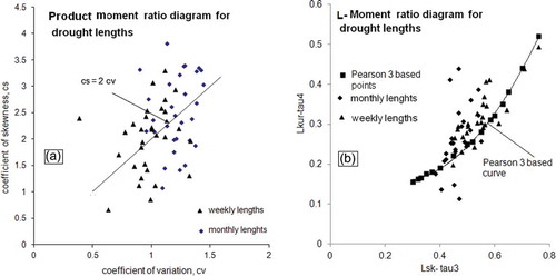
Although, a hypothesis of the Pearson 3 pdf (or gamma family) can be formed on the premise of geometric distribution of the successive occurrences of wet and drought periods, it is prudent to make a preliminary assessment of the pdf of L values spanning the drought events. A simple approach involves the assessment of the product moment ratio diagram, where the coefficient of variation (cv as abscissa) and the skewness (cs as ordinate) are graphically displayed. Since, cs = 2cv for the gamma family, the scatter of points is expected to plot on the line with a slope of 2. At the monthly and weekly time scales, therefore, the cv and cs of L values from all five rivers were computed at q levels of 0.5, 0.4, 0.3, 0.2 and 0.1, and product moment diagrams were plotted. Although, the scatter of data points is relatively dispersed in the product moment diagram (Fig 2(a)), there is a tendency for data points to plot nearly in a balanced fashion on both sides of the line (cs = 2 × cv). The behaviour of drought lengths to obey the Pearson 3 pdf was further examined using the L-moment ratio diagram. The L-moments for the drought lengths were computed following the algorithms documented in Vogel and Fennessey (1993) and Hosking and Wallis (1997). The graphs between L-kurtosis (Lkur) as ordinate and L-skewness (Lsk) as abscissa were plotted (Fig 2(b)). The points, on both a monthly and a weekly basis, plotted reasonably well on both sides of the theoretical curve for Pearson 3 (Lkur-tau4 versus Lsk-tau3). The L-moment graph therefore vindicates the hypothesis of drought lengths to obey the Pearson 3 pdf (i.e. the gamma family).

Fig. 2 (a) Product moment and (b) L-moment diagrams for drought lengths in the Canadian prairies.

4.1 Return periods (T_r) of drought lengths using various pdfs

The Bow River has been used as an illustrative example to predict return periods of drought lengths using various pdfs. The parameters of pdfs corresponding to the Pearson 3, the gamma, the exponential, and the Weibull 3 and Weibull distributions were estimated using the MOM. For example, at q = 0.3, n_s = 567, s² = 11.03, cs = 3.29, θ = 0.11; using these statistics, values of relevant parameters of various distributions are calculated, as shown in Table 4. Plugging these values into equations (10) to (13), the values of T_r were computed for L = 2, 3, 4, …, 27 (L_max = 27 in the observed data). The value of T_r for L = 1 was not computed as this would cause the integration in a three-parameter situation to be undefined. Moreover, this computation makes little difference in the assessment on the quality of fitting rendered by various distributions. Likewise, at all q levels (0.5, 0.45, 0.40, 035, 0.3, 0.25, 0.2, 0.15 and 0.10), the values of T_r were computed for comparative analysis with the observed counterparts.

Table 4 Summary of predicted return periods (T_r) at varying drought lengths (L_r) in weeks using various pdfs (at q = 0.3, T = 5252 weeks) for the Bow River.

L (n) week	Tr-ob week	Pearson 3		Weibull 3		Exponential		Gamma		Weibull
		Para.*	Tr	Para.	Tr	Para.	Tr	Para.	Tr	Para.	Tr
2 (271)	19	λ = 0.21	21	u = 2.13	24	λ = 2.80	19	λ = 0.71	21	u = 2.56	21
3 (178)	30		31		37		27		29		29
4 (128)	41	β = 5.46	42	k = 0.58	54	θ = 0.11	39	β = 3.94	39	k = 0.85	50
6 (73)	72		73		98		79		70		72
8 (41)	128	ε = 1	122	ε = 1	162		162	θ = 0.11	123	θ = 0.11	127
10 (27)	195	θ = 0.11	196	θ = 0.11	253		331		214		219
12 (21)	250		311		379		676		370		371
14 (9)	584		486		552		1382		638		621
16 (6)	875		753		784		2821		1093		1027
18 (5)	1050		1157		1093		5774		1868		1682
20 (5)	1050		1767		1499		11803		3185		2732
22 (4)	1313		2685		2028		24127		5416		4405
24 (2)	2626		4063		2711		49320		9195		7054
27 (1)	5252		7515		4110		144147		20278		14137

* Para. denotes parameters.

The quality of fit in each case of various pdfs was evaluated using statistics commonly-used in hydrological analyses, such as the coefficient of efficiency (COE) and the mean error of prediction (ME), both expressed in percentage terms (Sharma and Panu 2010, 2012). From a review of Table 4 (pertaining to q = 0.30), it is apparent that: (a) at low values of L, almost all pdfs are able to estimate values of T_r that are relatively similar to their observed counterparts (T_r-ob, column 2); (b) with 1- to 2- parameter pdfs, the predicted values of T_r (columns 8, 10, 12) tend to diverge significantly as values of L become larger than 20; and (c) in the entire range of L, the three-parameter pdfs (viz. the Pearson 3 or the Weibull 3) tend to perform more consistently with less divergence in predicted values of T_r (columns 4 and 6) when compared to their observed counterparts. Similar trends were observed at other q levels mentioned above. Based on these observations and since extreme droughts refer to large L values, it is reasonable to conjecture that the three-parameter distributions are better suited to model return periods. Nevertheless, the efficacy in terms of the COE and ME of all five pdfs was tested. In turn, these pdfs were used to predict values of T_r for the Bow River involving aforesaid q levels at both weekly and monthly time scales.

While evaluating the statistics, it was kept in mind that the discrepancy between observed and predicted return periods at a given L should not be excessive. Such an observation is evident from a cursory review of values of return periods in Table 4. To elucidate the point, comparing the values in columns 2, 4 and 6, one could easily discover that when L exceeds 18 (or n = 5), the discrepancy between T_r and T_r-ob, becomes excessive in both Pearson 3 and Weibull 3 pdfs. A similar trend was displayed by other pdfs under investigation. One reason for such wild divergence can be attributed to small n, which reflects the weak averaging effect on T_r-ob. Therefore, in this case, T_r-ob values ranging from l9 (L = 2) to 1050 (L = 18), or n = 5 (as the lower cut-off point for the number of runs), were involved in the assessment of performance statistics. Other values of T_r-ob and corresponding T_r (predicted values) were not included in the evaluation of performance statistics. At each q level and the weekly time scale, these limits of T_r-ob will fluctuate roughly within the range 19–1050. Corresponding to these values of T_r-ob, the minimum value of n was found to be 4 in almost all q levels for the rivers under consideration. At a monthly time scale, these limits of T_r-ob were found to fluctuate between 10 and 606 for all q values considered, with a cut-off of n = 4. The resulting performance statistics are summarized in Table 5.

Table 5 Summary of performance statistics using various pdfs for the evaluation of return periods (T_r) in weeks or months of varying drought lengths (L_r) for the Bow River. COE: coefficient of efficiency; ME: mean error of prediction.

Statistic	Pearson 3		Weibull 3		Exponential		Gamma		Weibull
	Week	Month	Week	Month	Week	Month	Week	Month	Week	Month
COE (%)	96.11 (96.54)*	95.11 (96.0)*	91.90	89.41	−3859.0	76.71	36.51	47.71	5.25	35.95
ME (%)	0.58 (0.24)*	1.07 (3.95)*	18.95	30.20	396.0	44.50	396.0	46.00	39.39	46.00

* statistics are based on cs estimates using equation (6); other values are based on cs using equation (5).

It is apparent from Table 5 that the 2-parameter (gamma and Weibull) and 1-parameter (exponential) distributions are relatively weak in predicting the behaviour of T_r and, therefore, were not considered for further analysis. The Pearson 3 distribution provides the best performance, followed by the Weibull 3 distribution. Although the value of COE is above 90% for the Weibull 3, there exists a tendency of over-prediction in the range of 19% or more. Therefore, the Pearson 3 and Weibull 3 distributions were retained for further analysis of return periods for the rivers considered in this study. In the case of the Pearson 3, two modes of estimation of cs were employed, namely equations (5) and (6), both of which resulted in nearly similar values of performance statistics due to large values of n_s for the Bow River. An important point worth noting in Table 5 is that the performance of the exponential pdf appears to be far less satisfactory, especially in view of the fact that in the past this distribution has been used as a dominant model for describing the pdf of drought lengths.

At the weekly and monthly time scales, and in view of the above analysis, summary tables similar to Table 4 were prepared for all five rivers at q levels ranging from 0.5 to 0.10 (with a step of 0.05). For the Churchill River, smaller values of n_s at q < 0.20 were not considered. The performance statistics COE and ME were evaluated for all five rivers at both weekly and monthly time scales, and are summarized in Table 6. The following observations can be made:

1. The MOM seems to be satisfactory for the estimation of parameters in the rivers under consideration, with exception of the Churchill River, because the sample size of drought spells (n_s) is small (< 30).

2. In general, the Weibull 3 distribution tends to over-predict return periods at both the weekly and monthly time scales.

3. Estimates of parameters in the Pearson 3 distribution based on the customary method of estimation of cs (equation (5)) tend to under-predict return periods (as shown by ^† in line 2 of each row for the river), except for the Bow River where the sample size is very large. In fact, for the Churchill River, the under-prediction is exceptionally large, probably due to the small sample size of drought spells.

4. Using the modified method of estimation of cs in equation (6), the under-prediction was ameliorated. The revised values of cs and the corresponding new estimates of parameters not only significantly reduced the under-prediction, but also resulted in a modest over-prediction (as shown by * in Table 6). The scenario of the Bow River changed insignificantly, probably in view of the large size samples of drought spells (n_s). However, the scenario of the Churchill River did not return to an acceptable level because values of COE still remained less than 80%.

5. The MML was employed to estimate the parameters in the Pearson distribution for the Churchill River, which significantly improved values of COE to a level of nearly 92% on a weekly scale and 97% at the monthly time scale. Although, values of COE improved significantly, a mild under-prediction (≈–4%, Table 6) was found to occur at the weekly time scale. At the monthly time scale, however, there was a tendency for a mild over-prediction (≈1.50%). Since, the MML performed reasonably well for the Churchill River, its efficacy was also tested on other rivers. It turned out that the MML method did not perform well and only resulted in diminished values of COE and further, at times, resulted in negative values. At the weekly time scale, a case in point is the Bow River, in which the resulting value of COE was –93.16%, with ME of 37.12%; at the monthly time scale, COE was found to be 3.55% with a ME of 6.35%. This observation illustrates that the MOM seems to be a preferable method for large samples, where the MML may tend to outperform. However, the MML appears to be more suitable for data-deficient scenarios, where the MOM is unable to provide estimates of parameters within an acceptable accuracy and certainty.

   Table 6 Summary of performance statistics in the evaluation of return periods (T_r) of varying lengths (L_r) for rivers in the Canadian prairies using the Pearson 3 and Weibull 3 pdfs.

   River	Pearson 3 (using MOM* & MML)				Weibull 3 (using MOM*)
   	Weekly		Monthly		Weekly		Monthly
   	COE (%)	ME (%)	COE (%)	ME (%)	COE (%)	ME (%)	COE (%)	ME (%)
   Athabasca
   ns = 40–83 (in month)	96.95	0.86	98.07	3.81	96.95	11.65	93.06	24.41
   ns = 69–226 (in week)	(98.77)^†	(−0.76)^†	(97.76)^†	(−3.34)^†
   Beaver
   ns = 34–52 (in month)	97.13	1.20	94.39	4.86	84.05	30.97	80.04	24.25
   ns = 67–113 (in week)	(98.25)^†	(−5.11)^†	(96.21)^†	(−10.41)
   Bow
   ns = 73–185 (in month)	96.54	0.24	96.00	3.95	91.90	18.95	89.41	30.20
   ns = 297–672 (in week)	(96.11)^†	(0.58)^†	(95.11)^†	(1.07)^†
   South Saskatchewan
   ns = 34–76 (in month)	97.75	−0.51	91.61	2.26	89.07	20.62	69.97	27.03
   ns = 111–235 (in week)	(97.74)^†	(−1.46)^†	(89.92)^†	(−6.47)^†
   Churchill
   ns = 14–20 (in month)	91.89^‡	1.0^‡	97.08^‡	−3.48^‡	83.99	6.40	35.70	25.18
   ns = 20–26 (in week)	(77.66)	(4.65)	(78.26)	(8.42)
   q ≥ 0.2 for both times	(79.26)^†	(−26.89)^†	(53.09)^†	(−38.19)^†

   * (cells without an identifier) values are MOM-based parameters with revised values of cs using equation (6).

   ^† values are based on the parameters (MOM) computed with estimates of cs using equation (5).

   ^‡ values are based on the MML.

Based on the above analysis, it can be concluded that the Pearson 3 is an appropriate pdf for computing the behaviour of return periods of hydrological drought lengths in the Canadian prairies. The MOM, using the method of Bobee and Robitaille (1977), was found to be superior for obtaining the estimate of cs. For highly persistent flows, such as those displayed by the Churchill River, the MML is more suitable for estimating parameters of the Pearson 3 pdf. The Weibull 3 pdf tended to significantly over-predict return periods and therefore is less suitable for the prediction of return periods of hydrological droughts in the Canadian prairies.

4.2 Linkages between return periods (T_r) and the sampling period (T) of SHI sequences

As return periods respond well with the Pearson 3 pdf at monthly and weekly time scales, the same pdf can be utilized to predict return periods of hydrological droughts at the annual time scale. One can consider the case of the Bow River, where there is a record of 101 years; using levels of q = 0.5, 0.45, 0.40, 0.35, 0.30, 0.25, 0.20, 0.15, 0.10 and 0.05 (at a step of 0.05), the recorded L_max were respectively found to be 7, 7, 5, 4, 3, 3, 3, 2, 2 and 2 years. The corresponding values of T_r (using equations (10) and (11) relevant to the Pearson 3 pdf with ε = 1) were found to be 132, 225, 202, 101, 40, 95, 237, 163, 266 and 298 years, with a mean value of 174 years. The longest drought observed in the historical flow record only lasted for 7 years (2000–2006) with a value of q = 0.5 and, therefore, should be construed as having a return period of 176 years. This value of return period compares well with 181 years estimated by the Gringorten (1963) formula. Similar investigations were repeated for other rivers and corresponding results are summarized in Table 7. Likewise, a drought persisted for 6 years (1956–1961) in the Athabasca River, for which a return period of 118 years was estimated by the Pearson 3 method; this compares well with the return period of 120 years estimated by the Hazen formula. It is noted that more than 10 probability levels were discernible in only two rivers, namely the Athabasca and the Bow, at the annual time scale in terms of number of spells (n_s) that could result in meaningful estimates of parameters. In the case of the Beaver and Churchill rivers, n_s ≤ 2 was observed at q < 0.2, which is too small for calculating the parameters. Likewise for the Saskatchewan River, the cut-off level of q was 0.15. So the calculations for the above three rivers are based on q ≥ 0.15.

Table 7 Comparison of return periods (T_r) using the Pearson 3 pdf of L_max (historically recorded) with empirically derived return periods for rivers in the Canadian prairies.

River	Annual time scale			Monthly time scale			Weekly time scale
	T year	Tr year	Closest formula	T month	Tr month^†	Closest formula	T week	Tr week	Closest formula
Athabasca	60	118	120 (Hazen)	720	731 (1.5%)	Weibull	3120	3540 (13%)	Weibull
Beaver	55	100	98 (Gringorten)	660	743 (13%)	Weibull	2860	2945 (3%)	Weibull
Bow	101	176	181 (Gringorten)	1212	1250 (3%)	Weibull	5252	5585 (6%)	Weibull
S. Sask.	52	87	91 (Gringorten)	624	683 (9%)	Weibull	2704	2779 (3%)	Weibull
Churchill	48	106	96 (Hazen)	576	613* (6%)	Weibull	2496	2851* (14%)	Weibull

S. Sask.: South Saskatchewan.

* the estimate is based on the MML.

^† values in parentheses indicate the percentage by which the return period is greater than the sample size.

Computations similar to the above were also carried out at monthly and weekly time scales to estimate the T_r for L_max that was observed in the record of T weeks or T months. However, an issue emerged in the selection of the correct value of L_max. For example, at q = 0.5 for the Bow River, L_max = 20 months and the next observed maximum length is L_max = 17 months. This observation implies that all values of 18, 19 and 20 months can be deemed equivalent to L_max and any one of them can be used to compute T_r subject to the constraint that the estimated T_r closely matches the sample size T. In the case of the Bow River L_r = 20, T_r = 2166; for L_r = 19, T_r = 1640; for L_r = 18, T_r = 1240 (units of L_r and T_r in months). Therefore, for comparative analysis, the value of L_max = 18 months will be used in the computation to yield T_r = 1240 months, because this value is closest to the value of T = 1212 months. Table 7 summarizes results of computations of return periods for all the five rivers using q = 0.5 to 0.05 with a step of 0.05 (at monthly and weekly time scales).

It is apparent from values in Table 7 that T_r is represented well by the Hazen (1930) or the Gringorten (1963) empirical plotting position formulae on the annual time scale. At the monthly or weekly time scales, the computed T_r is 1.5–14% greater than sample size T and yet the closest correspondence is given by the Weibull plotting position formula (return period = T + 1). In recent studies, Sharma and Panu (2010, 2012) assumed a sampling period T equivalent to T_r on monthly and weekly time scales in the context of MC models (MC-0, MC-1, MC-2, respectively, representing Markov Chain models of order zero, one and two) as applied to Canadian hydrological droughts. The MC-1 (monthly) and MC-2 (weekly and sometimes on highly persistent monthly flows) performed well with the above assumption. On an annual time scale, the sample size being comparatively small (T < 101), they assumed T_r to be twice the value of T (Hazen formula), which resulted in the satisfactory predictions by the MC-0 or MC-1 model. In short, the analysis based on the Pearson 3 pdf, as demonstrated in this paper, corroborates the hypotheses regarding the return period used in the MC methodology for estimating drought lengths by these authors.

It is worth reporting that Weibull, Hazen and Gringoten plotting position formulae, despite being old, have not only proven to be reliable in predicting the return periods of floods (Adamowski 1985, Moon and Lall 1994), but also compare well with return periods of drought durations (Kim et al. 2003). In almost all non-parametric approaches dealing with analysis of return period, these plotting position formulae have played significant and important roles in the development of algorithms and also validating the results pertaining to return periods.

5 Conclusions

Based on the analysis of the streamflow data from five rivers in Canadian prairies, with a database of 48–101 years, it can be concluded that the Pearson 3 probability distribution is a suitable distribution for describing the characteristics of return periods for drought lengths at varying truncation levels expressed in terms of drought probabilities (q). The location parameter ε can be set (= 1 year or 1 month or 1 week) based on the respective time scale, and the parameters λ and β can be estimated by the MOM for large drought event sample sizes (>30). The estimates of skewness (cs) in the MOM should be obtained involving the correction factor recommended by Bobee and Robitaille (1977). For a small sample size of drought events (<30), it is advisable to use the MML. The study indicated that the return period of the largest drought length computed by the Pearson 3 pdf compares well with the Hazen or the Gringorten empirical (plotting position) formulae at the annual time scale and the Weibull formula at the monthly and weekly time scales.

Disclosure statement

No potential conflict of interest was reported by the author(s).

Additional information

Funding

The partial financial support of the Natural Sciences and Engineering Research Council of Canada for this project is gratefully acknowledged.

REFERENCES

- Adamowski, K., 1985. Nonparametric kernal estimation of flood frequencies. Water Resources Research, 21 (11), 1585–1590. doi:10.1029/WR021i011p01585
- Bayazit, M. and Önöz, B., 2005. Probabilities and return periods of multisite droughts. Hydrological Sciences Journal, 50 (4), 605–615. doi:10.1623/hysj.2005.50.4.605
- Bobee, B. and Robitaille, R., 1977. The use of the Pearson type 3 and log Pearson type 3 distributions revisited. Water Resources Research, 13 (2), 427–443. doi:10.1029/WR013i002p00427
- Bonaccorso, B., Cancelliere, A., and Rossi, G., 2003. An analytical formulation of return period of drought severity. Stochastic Environmental Research and Risk Assessment (SERRA), 17 (3), 157–174. doi:10.1007/s00477-003-0127-7
- Bonaccorso, B., et al., 2012. Large-scale probabilistic drought characterization over Europe. Water Resources Management. doi:10.1007/s11269-012-0177-z
- Cancelliere, A. and Salas, J.D., 2004. Drought length properties for periodic hydrologic data. Water Resources Research, 10 (2), 1–13.
- Cancelliere, A. and Salas, J.D., 2010. Drought probabilities and return period for annual streamflows series. Journal of Hydrology, 391, 77–89. doi:10.1016/j.jhydrol.2010.07.008
- Chow, V.T., Maidment, D.R., and Mays, L.W., 1988. Applied hydrology. New York: McGraw-Hill.
- Environment Canada., 2011. HYDAT CD-ROM Version 96-1.04 and HYDAT CD-ROM User’s Manual. Surface Water and Sediment Data. Water Survey of Canada.
- Fernández, B. and Salas, J.D., 1999a. Return period and risk of hydrologic events. I: mathematical formulation. Journal of Hydrologic Engineering, 4 (4), 297–307. doi:10.1061/(ASCE)1084-0699(1999)4:4(297)
- Fernández, B. and Salas, J.D., 1999b. Return period and risk of hydrologic events. II: applications. Journal of Hydrologic Engineering, 4 (4), 308–316. doi:10.1061/(ASCE)1084-0699(1999)4:4(308)
- González, J. and Valdés, J.B., 2003. Bivariate drought recurrence analysis using tree ring reconstructions. Journal of Hydrologic Engineering, 8 (5), 247–258. doi:10.1061/(ASCE)1084-0699(2003)8:5(247)
- Gringorten, I.I., 1963. A plotting rule for extreme probability paper. Journal of Geophysical Research, 68 (3), 813–814. doi:10.1029/JZ068i003p00813
- Haan, C.T., 1977. Statistical Hydrology. Ames: Iowa state University Press.
- Hazen, A., 1930. Flood flows, A study of frequency and magnitudes. New York: John Wiley and Sons.
- Hosking, J.R.M. and Wallis, J.R., 1997. Regional frequency analysis: an approach based on L-moments. Cambridge: Cambridge University Press, 191–209.
- Kendall, D.R. and Dracup, J.A., 1992. On the generation of drought events using an alternating renewal-reward model. Stochastic Hydrology and Hydraulics, 6 (1), 55–68. doi:10.1007/BF01581675
- Kim, T.-W., Valdés, J.B., and Yoo, C., 2003. Nonparametric approach for estimating return periods of droughts in arid regions. Journal of Hydrologic Engineering, 8 (5), 237–246. doi:10.1061/(ASCE)1084-0699(2003)8:5(237)
- Kite, G.W., 1988. Frequency and risk analysis in hydrology (revised). Fort Collins, CO: Water Resources Publications.
- Koutrouvelis, I.A. and Canavos, G.C., 1999. Estimation in the Pearson type 3 distribution. Water Resources Research, 35 (9), 2693–2704. doi:10.1029/1999WR900174
- Lana, X., et al., 2006. Statistical distributions and sampling strategies for the analysis of extreme dry spells in Catalonia (NE Spain). Journal of Hydrology, 324, 94–114. doi:10.1016/j.jhydrol.2005.09.013
- Lana, X., et al., 2008. Return period maps of dry spells for Catalonia (northeastern Spain) based on the Weibull distribution. Hydrological Sciences Journal, 53 (1), 48–64. doi:10.1623/hysj.53.1.48
- Matalas, N.C. and Wallis, J.R., 1973. Eureka! It fits a Pearson type: 3 distribution. Water Resources Research, 9 (2), 281–289. doi:10.1029/WR009i002p00281
- Mathier, L., et al., 1992. The use of geometric and gamma-related distributions for frequency analysis of water deficit. Stochastic Hydrology and Hydraulics, 6, 239–254. doi:10.1007/BF01581619
- Millan, J. and Yevjevich, V., 1971. Probabilities of observed droughts. Fort Collins, CO: Colorado State University, Hydrology Paper 50.
- Moon, Y. and Lall, U., 1994. Kernel quantite function estimator for flood frequency analysis. Water Resources Research, 30 (11), 3095–3103. doi:10.1029/94WR01217
- Salas, J.D., et al., 1997. Applied modelling of hydrologic time series. Fort Collins, CO: Water Resources Publications.
- Salazar, P.G. and Yevjevich, V., 1975. Analysis of drought characteristics by the theory of runs. Fort Collins, CO: Colorado State University, Hydrology Paper 80.
- Şen, Z., 1980. Statistical analysis of hydrological critical droughts. Journal of Hydraulics ASCE, 1064 (HY1), 99–115.
- Şen, Z., 1989. The theory of runs with applications to drought prediction- comment. Journal of Hydrology, 110, 383–391.
- Şen, Z., 1990. Critical drought analysis by second order Markov chain. Journal of Hydrology, 120, 183–202. doi:10.1016/0022-1694(90)90149-R
- Şen, Z., 1999. Simple risk calculations in dependent hydrological series. Hydrological Sciences Journal, 44 (6), 871–878. doi:10.1080/02626669909492286
- Sharma, T.C. and Panu, U.S., 2008. Drought analysis of monthly hydrological sequences: a case study of Canadian rivers. Hydrological Sciences Journal, 53 (3), 503–518. doi:10.1623/hysj.53.3.503
- Sharma, T.C. and Panu, U.S., 2010. Analytical procedures for weekly hydrological droughts: a case of Canadian rivers. Hydrological Sciences Journal, 55 (1), 79–92. doi:10.1080/02626660903526318
- Sharma, T.C. and Panu, U.S., 2012. Prediction of hydrological drought durations based on Markov chains: case of the Canadian prairies. Hydrological Sciences Journal, 57 (4), 705–722. doi:10.1080/02626667.2012.672741
- Shiau, J.T., 2006. Fitting drought duration and severity with two-dimensional copulas. Water Resources Management, 20, 795–815. doi:10.1007/s11269-005-9008-9
- Shiau, J.T. and Shen, W.S., 2001. Recurrence analysis of hydrological droughts of different severity. Journal of Water Resources Planning and Management ASCE, 127 (1), 30–40.
- Vogel, R.M. and Fennessey, N.M., 1993. L-moment diagrams should replace product moment diagrams. Water Resources Research, 29 (6), 1745–1752. doi:10.1029/93WR00341
- Yevjevich, V., 1967. An objective approach to definitions and investigations of continental hydrologic droughts. Fort Collins, CO: Colorado State University, Hydrology Paper 23.
- Yevjevich, V., 1972. Stochastic processes in hydrology. Fort Collins, CO: Water Resources Publications.
- Zelenhasić, E. and Salvai, A., 1987. A method of streamflow drought analysis. Water Resources Research, 23 (1), 156–168. doi:10.1029/WR023i001p00156