Estimation of suspended sediment concentration in the Saint John River using rating curves and a machine learning approach

ABSTRACT

Sedimentation in navigable waterways and harbours is of concern for many water and port managers. One potential source of variability in sedimentation is the annual sediment load of the river that empties in the harbour. The main objective of this study was to use some of the regularly monitored hydro-meteorological variables to compare estimates of hourly suspended sediment concentration in the Saint John River using a sediment rating curve and a model tree (M5ʹ) with different combinations of predictors. Estimated suspended sediment concentrations were multiplied by measured flows to estimate suspended sediment loads. Best results were obtained using M5ʹ with four predictors, returning an R² of 0.72 on calibration data and an R² of 0.46 on validation data. Total load was underestimated by 1.41% for the calibration period and overestimated by 2.38% for the validation period. Overall, the model tree approach is suggested for its relative ease of implementation and constant performance.

EDITOR M.C. Acreman; ASSOCIATE EDITOR B. Touaibia

KEYWORDS:

• suspended sediment
• model
• model tree
• machine learning
• regression
• sediment rating curve

Introduction

Accurate sediment transport modelling is an important tool in many aspects of water resources management, such as water quality, fish habitat, dam design and operations. High concentrations of suspended sediment are known to have major consequences on river ecology including obstruction of light penetration, which is essential for primary production, or the silting of the substrate potentially altering the quality of salmonid spawning habitat and even preventing fry emergence (Wood and Armitage 1997).

Suspended sediment, representing most of the total amount of sediment transported downstream and being easier to monitor than other components (Meade et al. 1990), is commonly used to estimate sediment loads within a stream (Knighton 1998). To remain suspended in the water column, the upward velocity of the current induced by turbulence needs to be greater than the settling velocity of the particles. This settling velocity is essentially a function of particle density and size. The finer fraction of the sediment transported in the water column is referred to as wash material. Wash material is commonly associated with sediment smaller than 63 μm (clay and silt) which is carried by the flow over long distances (Asselman 2000, Church 2006). The other component of suspended sediment is bed material and represents the coarser fraction of the material that can be transported in suspension in the water column.

Part of the bed material is transported downstream through bedload processes such as rolling, sliding and saltation. The resuspension of the bed material depends on the hydraulic properties of the river, flow and sediment morphology. Bedload and dissolved solids are not accounted for in most analyses and will not be quantified in the present study. Wash material and bed material were measured simultaneously through turbidity monitoring and hence were not separated. We therefore use the term suspended sediment, which includes all solid material transported in suspension in the water column.

Factors controlling the amount of suspended sediment in a system can be divided into three categories (Onderka et al. 2012): hydrological, meteorological and physiographic. While hydrological (e.g. discharge, amplitude and timing) and meteorological (e.g. rain, snowmelt and wind) variables are widely available and easy to analyse, some physiographic factors such as land use and soil properties are harder to include in a short-term (i.e. daily or sub-daily time steps) predictive model. Although processes linked to suspended sediment transportation have been studied for many years, the contribution of these processes in predicting suspended sediment concentrations (SSC) over a short time period (sub-daily) remains poorly understood.

Several statistical methods have been developed to estimate SSC, ranging from basic sediment rating curves (SRC) to more complex models such as support vector regressions (Gao 2008, Kisi 2012). While SRC were proven to be effective in estimating SSC based on daily discharge measurements in some systems (Asselman 2000, Horowitz 2003), the complexity of the sediment dynamics sometimes requires more sophisticated approaches to explain most of the variability in SSC (Gao 2008). The main advantage of using data-driven models for suspended sediment transport modelling is their ability to deal with more complex dynamics than the simpler linear models. Machine learning approaches such as artificial neural networks (ANN), support vector regression, regression trees and model trees are increasingly used in suspended sediment prediction (Bhattacharya and Solomatine 2006, Shiri and Kişi 2012) and can offer a good alternative to classic approaches such as linear or deterministic models. Use of ANNs is now common in hydrology studies (e.g. stage–discharge rating curves, flow forecasting, etc.) and they are gaining popularity in sediment prediction (Cigizoglu 2004, Kisi et al. 2008). Another method, called model trees (MT), has been marginally used in sediment modelling but appears to yield results comparable to those obtained from an ANN, while being less complex to use. In its final form, a MT is a set of simple linear equations, which are easier to analyse than the results from an ANN (Bhattacharya et al. 2007, Mount and Abrahart 2012).

One major concern related to suspended sediment loads is the subsequent downstream deposition in ports, which may impede navigation of large commercial vessels (Bhattacharya and Solomatine 2006, Higgins et al. 2011). The Saint John Port Authority (SJPA) dredges sediments in the Saint John harbour (New Brunswick, Canada) every year to maintain a navigable channel. Although dredging is conducted annually, the amount of sediment removed from the harbour bed varies considerably from year to year. For example, in 1998, 52 791 m³ of sediment were removed from the harbour compared to 375 790 m³ in 2006, which is more than seven times the amount dredged in 1998 (SJPA, personal communication). One potential source of variability is the annual sediment load coming from the watershed through the Saint John River (SJR). Local resuspension in the estuary, caused by high tides in the Bay of Fundy, has also been identified as a potential source of sediment. The present study only focuses on the particles transported by the river.

Studies on suspended sediment mobilization in the SJR have been very sparse. Beltaos and Burrell (2000) measured SSC during ice breakup in the upper Saint John. Previous work on the SJR watershed has been completed by Higgins et al. (2011), who used an ANN model to simulate historical daily sediment loads in the Kennebecasis River, a tributary of the SJR. Their model had a good ability to estimate daily loads from mean air temperature, one- and two-day lagged discharge and day of the year as predictors, but the attempt to model hourly SSC returned poor results (Higgins 2010). Considering the lack of information on this topic in general, and specifically in the SJR, the present paper focuses on estimating hourly SSC in the SJR with the ultimate goal of calculating a total load for a given period of time.

A basic regression method, the SRC, and a more complex algorithm, the M5ʹ model tree, were both tested to estimate hourly SSC in the SJR and, ultimately, to calculate loads. A better performance by the M5ʹ model would justify its application, in spite of the fact that it is a somewhat more complex model than the SRC.

The objectives of the present paper are to:

1. Investigate which regularly monitored hydro-meteorological variables may be good predictors of SSC in the SJR;

2. Compare the SRC and the M5ʹ algorithm to estimate hourly SCC based on the selected predictors;

3. Suggest a model to estimate suspended sediment using commonly monitored variables to compensate in part for the lack of a suspended sediment monitoring programme in the SJR.

Methodology

Study area

The SJR watershed, from its headwaters in the State of Maine (USA) to its estuary in the Bay of Fundy (Canada), drains an area of roughly 55 000 km². Mean discharge is approximately 1100 m³/s (Cunjak and Newbury 2005). Mean current velocity recorded during summer 2011 and 2012 was 0.32 m/s with maximum velocity of 0.7 m/s and minimum velocity of 0.08 m/s. A number of factors, including extreme flood tides during low flows, may explain the very low recorded velocities. Average annual precipitation in Fredericton (Environment Canada Station 8101500) is about 1078 mm (1981–2010), 23% of which falls as snow. Three dams alter the natural flow of the SJR (Mactaquac, Beechwood and Grand Falls) and two other dams have been constructed on two major tributaries in the upper (northern) part of the basin: the Tobique and the Aroostook rivers. The SJR watershed is covered by forest (83%), agriculture (6%) and urban areas (2%). The region between Little River and Aroostook River along the main stem (350 km from the mouth of the river) is known to be an important source of sediment in the SJR watershed (Kidd et al. 2011) due to intensive potato farming.

Monitoring and sites

The use of turbidity as a surrogate for SSC is now widely accepted in suspended sediment analysis (Lewis 1996, Davies Colley and Smith 2001, Schoellhamer and Wright 2003). An autonomous probe (YSI OMS600) equipped with a turbidity sensor (YSI 6136) was installed in the lower part of the SJR near Maugerville, NB (Fig. 1). The instruments were attached to a buoy at one end and to a heavy anchor structure on the river bed and positioned 4 m from the bottom. Mean total depth during the monitoring period was 5.2 m. This installation was moored close to the channel during the summers of 2011 (30 June–18 November) and 2012 (4 May–21 August). A tipping bucket rain gauge (Onset) was also installed in an open field close to the site. The drainage area at the monitoring site is about 42 668 km² (Higgins 2010).

Figure 1. Study site map.

Calibration of turbidity meters

Because of many factors affecting light scattering in a natural environment, such as particle size, colour and shape, turbidity should not be used without a good knowledge of its relation with SSC at the monitoring site (Lewis 1996). Therefore, a calibration curve was built to relate turbidity values to SSC. Water samples were collected along a cross-section of the river on 18 July 2012 using a 500 ml integrated water sampler. Six sampling sites, evenly spaced along the river cross-section, were established. Two integrated water samples were collected at each site, then transferred into 500 ml bottles and stored at 4°C for two days before they were filtered. Filtration followed the protocol described by Edwards and Glysson (1999). Since we did not have access to an automatic water sampler and we have not been able to sample any major transport event by manual sampling, no extremely high turbidity values could be related to SSC from grab samples. Therefore, an alternative calibration method was developed based on the work of Pavey et al. (2007). Three grab sediment samples were collected from the riverbed close to the turbidity meter and analysed in a particle analyser (Malvern). Average D₅₀ value of the particle size distribution of the bottom sediment samples was 8.99 µm while D₉₀ was 53.33 µm. Thus, over 90% of the bottom sediment particles sampled in Maugerville were smaller than 63 µm. This is consistent with D₉₀ suggested by Walling and Moorehead (1989) for a similar watershed. Another river bed sample was subsequently taken at the same location and sieved using a 62 μm mesh size to save the finer fraction. The sample was brought to the lab and the sediments were separated from the water using a centrifuge. Water was then transferred into a 1000 ml graduated cylinder and turbidity was measured using the YSI sensor. The turbidity value was recorded and a first sample from the graduated cylinder was saved. Gradually, sediments were added to the water solution to increase turbidity. The turbidity level was recorded for each sample, which was then saved for subsequent filtering. It was difficult to concentrate a sufficient quantity of sediments in the laboratory to reach peak field turbidity values. Hence, the calibration interval was 0–830 NTU while monitored turbidity ranged from 1 NTU to 1170 NTU. However, values greater than 830 NTU represent only 0.9% of the field measurements and they are the only values estimated by extrapolation of the calibration curve (Fig. 2).

Figure 2. Calibration curve relating turbidity to SSC.

Data

The candidate SSC predictors were first selected based on their relevance to SSC from the literature (Robert 2003, Higgins et al. 2011, Onderka et al. 2012) and their availability. Rainfall was measured every 15 minutes, water levels were obtained from the Hydrological Survey of Canada, and hourly wind speed was obtained from the nearest Environment Canada meteorological station (station 8101500; Fig. 1). The dependent variable, i.e. turbidity (subsequently converted to SSC), was measured every 15 minutes. Hourly maxima, minima and means were calculated for all variables. The discharge used in the analysis is the sum of the discharge measured at the Mactaquac Dam and discharge measured by Environment Canada in the Nashwaak River (station 01AL002; Fig. 1). An area ratio was used to transfer the flow downstream, thereby accounting for the location of the monitoring station in the Nashwaak watershed. Hourly discharge was multiplied by hourly SSC to calculate hourly observed loads.

Correlation analysis for the selection of predictors

From the original variables, six other variates were calculated in an attempt to account for the fact that hydro-meteorological phenomena that may lead to high SSC may be temporally lagged with high SSC. The timing of SSC response to a precipitation event depends on many controlling factors, such as vegetation cover, slope of the basin, soil type, etc. In order to choose the time lag of the input variables, correlograms were built to assess lagged correlations between SSC and rain, and SSC and water level (Fig. 3). The Pearson correlation coefficient was used to find the strongest correlation between SSC and lagged water level (WL) ranging from 1 h to 600 h. The highest correlation, i.e. r = 0.37, was found between lagged water level and SSC for a time lag of 240 h (10 days; Fig. 4). Water level was better correlated with SSC than discharge and was therefore used in the choice of an appropriate lag.

Figure 3. Correlograms for lagged water level and cumulated rain over various time spans.

Figure 4. Time series of SSC and water levels in Maugerville, NB.

For precipitation, correlograms were built for cumulative rain starting at t = 0 and summing rainfall over preceding days until t = 600 h prior (Fig. 3). This was done in order to correlate SSC with its corresponding rain event instead of hourly rain intensity. Again, Pearson correlation coefficients were calculated. Highest correlation (r = 0.24; Fig. 3) was found for rain cumulated over 459 h preceding SSC, but r values remained around 0.21 for lags between 400 h and 500 h. A time period of 408 h (17 days) has been chosen for cumulative rain because it corresponds to the beginning of the plateau of the correlogram. The correlograms also show an increase of the correlation coefficient for rain cumulated over 1 day (r = 0.09; Fig. 3). We therefore included rain accumulated over 24 h preceding the SSC measurement. The pre-selected potential explanatory variables are listed in Table 1.

Table 1. Preselected explanatory variables.

Variable	Units	Definition
Rain	mm	Rain intensity during the hour
Rain24	mm	Rain cumulated over the 24 h preceding the SSC measurement
Rain408	mm	Rain cumulated over the 408 h preceding the SSC measurement
Discharge	m^3/s	Mean discharge during the hour
Velocity	m/s	Mean water velocity during the hour
Wind_Speed	km/h	Mean wind speed during the hour
WL	m	Mean water level during the hour
WL24	m	Mean water level recorded 24 h preceding the SSC measurement
WL240	m	Mean water level recorded 240 h preceding the SSC measurement
WL408	m	Mean water level recorded 408 h preceding the SSC measurement
WL240-408	m	Difference between WL240 and WL408

Correlation analyses were performed for hourly data to select model inputs from the pre-selected candidate variables. Both Pearson and Spearman correlations were run on pre-selected variables. The Pearson correlation was used to test for a linear relation, while Spearman correlation was included to evaluate whether a nonlinear relation was observed. When a significant correlation between the variable and SSC was found (p-value ≤ 0.01), from either the Pearson or Spearman correlation analysis, the variable was kept as a potential predictor.

Discharge, water level and velocity have been smoothed using a moving average of 9 h to remove the part of their fluctuations induced by the management of the Mactaquac Dam. Although the Mactaquac Dam is a run-of-the-river type of dam, some daily hydropeaking occurs (NB Power, personal communication). The variations of discharge and water level that are not associated with the variability in meteorological conditions should not be included in the analysis.

Sediment rating curve

Rating curves have been widely used in sediment modelling and thoroughly discussed in the sediment literature since 1970. The method can be simply described as a nonlinear empirical relation between discharge and SSC or load at a given site (Walling 1977). Although many different versions of the SRC have been developed, SRC is generally represented by a power function to which a constant can be added, adjusted on discharge and SSC:

(1)

where Q represents discharge and a, b and c are parameters to be adjusted. See Asselman (2000) for more information on SRC.

M5ʹ model tree

The data-driven model was built using the M5primelab toolbox developed by Jekabsons (2003), based on the work of Wang and Witten (1997) and Quinlan (1992). The M5ʹ model is a combination of binary classifications of the dependent variable (defining tree branches) with multivariate linear models as the leaves (Wang and Witten 1997). First, a decision tree is built using a splitting criterion in order to classify the data into subsets by maximizing the variance between the subsets. To achieve this goal, nodes are defined based on standard deviation and every splitting possibility. All splitting combinations are assessed for every attribute in order to maximize the standard deviation reduction at the node. This step is performed by computing an expected error reduction (SDR) as described by Quinlan (1992):

(2)

where SD is the standard deviation, T is the set of data that reaches the node and T_i are the data resulting from the splitting. Splitting will continue until the SDR reaches a predetermined threshold, usually 5%, or if a minimum sub-sample size is reached at a node. Once the splitting is done, the linear regressions are simplified by testing whether removing an attribute reduces the estimated error at the node (backward stepwise regression). If it does, the attribute is removed from the regression (Quinlan 1992). When the model has finished with simplifying, the complex tree needs to be pruned by replacing certain nodes by leaves, starting at the leaves down to the roots. It has also been demonstrated that adding a smoothing process improves the prediction accuracy of the model tree (Frank et al. 1997), especially when trained on small samples (Quinlan 1992). This final step adjusts the regression at the leaves by taking into account the predicted value at the previous node. For more details on the model tree algorithm, see Witten and Frank (2005) and Quinlan (1992).

Two parameters were adjusted in order to optimize the adjustment of M5ʹ on the calibration data. The first is the minimum number of training data cases needed to form a node. A single node cannot be used to estimate fewer cases than the value attributed by the user. The default value given to the M5primelab toolbox is 4. The second parameter is a smoothing coefficient that controls the magnitude of the smoothing process. If the smoothing coefficient is large, the model will act like one node, while if it is zero, no smoothing will be performed. The value typically attributed to that parameter is around 15 (Witten and Frank 2005).

Both statistical models were tested using a split sample technique. The first 75% of the data were used for the calibration and the last 25% were used for the validation. M5ʹ has been tested on all possible combinations of predictors. For every combination, the performance indicators were calculated for both the calibration and the validation dataset.

Model performance indicators

Models were compared using three performance indicators: coefficient of determination (R²; equation (3)), relative bias (RB; equation (4)) and relative root mean square error (RRMSE; equation (5)).

(3)

(4)

(5)

Results

During the monitoring period, mean SSC was 54.34 mg/L with a peak of 1650 mg/L while mean discharge was 697 m³/s with a peak of 2950 m³/s. Mean monitored water level during summer 2011 and 2012 was 5.2 m. Nearly half of the total load (48.5%) was transported between hour 876 and hour 1535 (23 August 2011 and 19 September 2011). During that period, the highest water level rise over the course of a week (WL240-408) was 1.04 m and mean discharge was 1495 m³/s. The highest water level (6.7 m) preceding a major SSC event was recorded 240 h before the event (Fig. 4). It was the result of the greatest water level rise during the monitoring period (2.4 m over 7 days).

Variable selection

Two of the 11 potential predictors (Table 1) did not meet the selection criterion (p-value > 0.01; rain and wind speed) and were therefore removed from the input matrix (Table 2). Pearson correlation coefficients (r) showed a good relation between SSC and WL240-408 (r = 0.46), WL240 (r = 0.37) and Rain408 (0.2) while Spearman coefficients (ρ) indicated strong correlations between SSC and Velocity (ρ = 0.6), WL (ρ = 0.71), WL24 (ρ = 0.71) and WL240 (ρ = 0.53).

Table 2. Pearson correlation coefficients (r) and Spearman correlation coefficients (ρ) between SSC and explanatory variables.

Variable	r	p-value	ρ	p-value
Rain	−0.01	0.41	−0.03	0.02
Rain24	0.02	0.065	−0.04	0.003
Rain408	0.2	0.001	0.43	0.001
Discharge	0	0.807	0.42	0.001
Velocity	0.05	0.001	0.6	0.001
Wind_Speed	−0.01	0.561	0.02	0.1
WL	0.13	0.001	0.71	0.001
WL24	0.16	0.001	0.71	0.001
WL240	0.37	0.001	0.53	0.001
WL408	−0.03	0.016	0.22	0.001
WL240-408	0.46	0.001	0.27	0.001

All 511 possible combinations of the nine potential predictors obtained from the correlation analysis were provided as inputs to the M5ʹ algorithm and model performance in each case was assessed using the three performance indicators. Two types of SRC were also calibrated: SRC–Q—the most common model using discharge as a predictor, and SRC–WL240-408—a rating curve that used the difference between water level recorded 240 h and 408 h prior to SSC (WL240-408) as the independent variable.

Model performances

SRC

The SRC using discharge as a predictor of SSC (SRC–Q) returned null R² for the calibration period and consequently the model made a poor estimate of the SSC for the validation dataset (Fig. 5(a)). SRC–WL240-408 (i.e. using WL240-408 as the predictor) also returned a null R² on the calibration dataset but, surprisingly, it was able to explain 55% of the variance of the validation dataset (i.e. R² = 0.55; Fig. 5(a)). Despite the low R², SRC–WL240-408 returned RRMSE of 0.08 on calibration data and 0.10 on validation data. Figure 5 shows that SRC–WL240-408 was able to predict three of the four major transportation events, which could not be done by SRC–Q, although both rating curves systematically underestimate SSC.

Figure 5. Observed and estimated SSC using: (a) SRC–Q and SRC–WL240-408; (b) M5ʹ with 1 predictor; (c) M5ʹ with 3 predictors and (d) M5ʹ with 4 predictors.

M5ʹ

The M5ʹ model returned its best results when the minimum number of cases per branch was raised to 12 and the smoothing coefficient was lowered to 5. These values are coherent with the analysis of Witten and Frank (2005), which suggests that the minimum number of cases would need to “be increased for tasks that have a lot of noisy data”, as in the present study (Fig. 4). As for the smoothing coefficient, Witten and Frank (2005) stated that the smoothing process is more useful for models fitted on a small number of samples to prevent abrupt shifts in the estimated data. Thus, the relatively large dataset (n = 5566) of the present study may explain the better results associated with a lower smoothing coefficient.

In contrast with SRC–WL240-408, M5ʹ gave better results when tested on calibration data than when it was tested on validation data, with the exception of M5ʹ–1 pred. The results showed systematic overfitting when more than seven predictors were provided to M5ʹ, as indicated by the high R² obtained during calibration, but poor results on the validation dataset (R² = 0; Table 3). When M5ʹ was provided with four to seven predictors, models with similar performance were built, returning R² = 0.72 on calibration data for all four models and R² ranging from 0.45 (M5ʹ–7 pred.) to 0.47 (M5ʹ–5 pred.; Table 3) for the validation period. When the M5ʹ model was limited to using two and three predictors, both M5ʹ–2 pred. and M5ʹ–3 pred. explained a third of the variance during validation (R² = 0.36). M5ʹ–3 pred. yielded better calibration results (R² = 0.74) than M5ʹ–2 pred. (R² = 0.48). Three selected M5ʹ models are presented graphically in Fig. 5. It shows that M5ʹ–1 pred. and M5ʹ–3 pred. are better than M5ʹ–4 pred. at estimating the peak of the high SSC event during the validation period. On the other hand, M5ʹ–4 pred. estimated more precisely the duration of that event. We can also observe that estimated SSCs become less noisy when more predictors are provided to the algorithm.

Table 3. Results from the SRC models and from the best combination of predictors provided to M5ʹ.

Number of predictors	Calibration			Validation			Predictors
	R^2	RRMSE	RB	R^2	RRMSE	RB
SRC
1	0	0.63	0.51	0	0.15	0.03	Q
1	0	0.08	0.03	0.55	0.1	0.01	WL240-408
M5ʹ
1	0.21	0.06	0.0004	0.52	0.1	0.001	WL240-408
2	0.48	0.05	0.01	0.36	0.12	0.01	WL240-408–WL240
3	0.74	0.04	0.001	0.36	0.12	0.001	WL240-408–Rain408–Velocity
4	0.72	0.04	0.002	0.46	0.11	0.007	WL240-408–WL240–Rain408–Velocity
5	0.72	0.04	0.003	0.47	0.11	0.008	WL240-408–WL240–Rain408–WL24–Velocity
6	0.72	0.04	0.003	0.46	0.11	0.008	WL240-408–WL240–Rain408–WL24–WL–Velocity
7	0.72	0.04	0.003	0.45	0.12	0.008	WL240-408–WL240–Rain408–WL24–WL–Velocity–Q
8	0.77	0.04	−0.001	0	0.19	−0.03	WL240-408–WL240–Rain408–WL24–WL–Velocity–Rain24–Q
9	0.76	0.03	0.01	0	0.16	0.04	WL240-408–WL240–Rain408–WL24–WL–Velocity–WL408–Rain24–Q

Comparison of models

No model was able to adequately predict peak SSC values. Best estimation of high values (i.e. SSC > 900 mg/L) was given by M5ʹ –1 pred. and M5ʹ –3 pred. on validation data while estimation was better achieved by M5ʹ –3 pred. and M5ʹ –4 pred. during the calibration period (Fig. 5(b–d)). All M5ʹ models were better than the two SRC for simulating abrupt shifts from high to low SSC, especially on calibration data (Fig. 5). Similar RRMSE were observed for all three M5ʹ models on calibration (RRMSE ≤ 0.06) and validation data (RRMSE ≤ 0.12), while RRMSE was higher for SRC–Q and SRC– WL240-408 on both calibration (RRMSE = 0.63; RRMSE = 0.08) and validation data (RRMSE = 0.15; RRMSE = 0.1). All models showed a relative bias under 5% except for SRC–Q, which returned a relative bias of 51% on calibration data.

Loads

Once estimated with the five models, SSC were multiplied by mean observed hourly discharge to estimate loads, and cumulated for both the calibration and the validation period. The same has been done with observed SSC. The results are shown in Table 4. Surprisingly, the best total estimated loads for the calibration period were obtained using SRC–Q (0.01% above observed loads). M5ʹ–4 pred. also showed very small bias for the calibration period (1.41% underestimation). For the validation period, the best estimation of the total loads was obtained using M5ʹ–1 pred. (1.63% overestimation of observed loads) followed by M5ʹ–4 pred., overestimating loads by 2.38%. Although SRC–Q returned a good estimate of the total load for the calibration period, Fig. 6 clearly demonstates that this good estimate was the result of the underestimation of some cumulated load values counterbalanced by the overestimation of some other values. On Fig. 6, we can see that hourly load estimation was better achieved by M5ʹ–4 pred. compared to those estimated by SRC–Q. Figure 7 also shows that SRC–Q failed to stay close to the 1:1 line (representing perfect load estimation) for the whole period. M5ʹ–3 pred. and M5ʹ– 4 pred. both stayed fairly close to the 1:1 line for the calibration period. During the validation period, this was better achieved by M5ʹ–4 pred. and M5ʹ–1 pred.

Table 4. Loads calculated from observed SSC and estimated SSC.

Load (t)	Observed	SRC–Q	SRC–WL240-408	M5ʹ–1 pred.	M5ʹ–3 pred.	M5ʹ–4 pred.
Calibration
Total load (t)	670067	670152	582015	597013	656955	660636
Diff.	—	85	−88053	−73055	−13113	−9432
Diff. (%)	—	0.01	−13.14	−10.9	−1.96	−1.41
Validation
Total load (t)	82608	38987	75917	83955	95157	84574
Diff.	—	−43621	−6691	1346	12549	1966
Diff. (%)	—	−52.8	−8.1	1.63	15.2	2.38

Figure 6. Time series of hourly loads for SRC–Q and M5ʹ–4 pred.

Figure 7. Cumulated hourly loads calculated from observed SSC and estimated SSC: (a) on calibration data and (b) on validation data.

Discussion

A strong correlation was observed between predicted SSC and water level conditions 10 days before SSC measurements and rainfall amounts accumulated over 408 hours (Table 2). One possible explanation for the 10-day lag could be the slow response of the large catchment to a rain event. The concentration of suspended sediment typically depends on two parameters: the competence of the stream (the ability of a stream flow to mobilize sediment of a given size, Church 2006) and the sediment supply. In most rivers, SSC are not controlled by the competence of the stream, but mostly by the limited supply in sediment (Robert 2003, Ritter et al. 2006). This observation is one reason for the large scatter associated with SRCs, and might explain why such curves occasionally fail to adequately predict SSC, as in the present study (Gao 2008). This means that the lag between the hydrograph and the SSC peak is due to the travelling time between the sediment supply and the monitoring site. The region from Little River to Aroostook River along the SJR (220 km upstream from the monitoring site) is known to be an important source of sediment for the SJR watershed due to intensive potato farming (Kidd et al. 2011). Xing et al. (2011) have reported “soil losses ranging from 22 to 53 t/ha/yr” for the northern New Brunswick region located along the SJR. A portion of that region, known as the potato belt, has been targeted by Environment Canada and Agri-Food Canada to assess the impact of agriculture on water quality and aquatic communities (Benoy et al. 2012). The total area of the sub-basin is 254.9 km², with 41.2% cultivated land. If the soil loss rate reported by Xing et al. (2011) is applied to that sub-basin, it would represent a total soil loss of 231 041–556 600 t/year for what is only approximately 0.5% of the whole SJR watershed. The portion of the lost soil that reaches the river is unknown, but the important sediment yield suggests a strong influence of soil erosion associated with potato farming on SSC measured downstream in the SJR. Hence, considering that the potential sediment source is located more than 200 km upstream of the monitoring site, the 10-day time lag (r_WL240 = 0.37) may represent the time it takes for a particle to be eroded at its source, be carried through the watershed to the river, and finally reach the monitoring site.

For some streams, a counter-clockwise hysteresis loop can be observed “when sediment originates from a distant source or when the valley slopes form the most important sediment source” (Asselman 1999). Following the hypothesis that the above-mentioned agricultural region is the main source of sediment, the origin of the particles would be both distant and from the valley slope. Figure 8 shows that the hysteresis loop of the two main sediment transport events measured during our monitoring period showed counter-clockwise patterns. In both cases, water level (X axis) rises before SSC (Y axis) increases, thereby causing the SSC peak to happen in the falling limb of the hydrograph. Such observations have been reported in the past by many authors including Klein (1984), Bača (2008), and Smith and Dragovich (2009).

Figure 8. Hysteresis loops on daily data for the main events of the monitoring period: (a) hour 1208–1928 (8 August 2011–18 September 2011) and (b) hour 4520–5095 (21 June 2012–14 July 2012). A 3-day moving average has been performed to reduce noise.

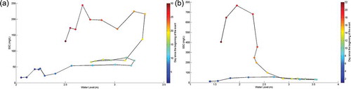
Other causes such as bank collapse after high discharge have been known to produce counter-clockwise patterns in hysteresis loops (Marttila and Kløve 2010), but no literature on the topic was available for the SJR drainage basin at the time of the present study. Given that peak current velocity during summers 2011 and 2012 was 0.7 m/s, and almost certainly faster during spring, it would take less than 4 days for a suspended particle to be transported from the agricultural area to our monitoring site. The flow of the SJR is altered by the presence of three dams between the sediment source and our site. Although they are all run-of-the-river type dams, their presence may be one possible explanation of the longer than expected lag between a rain event and the transportation of suspended sediment in Maugerville due to slower water velocity above the dams. Therefore, the lagged water level is likely more of a proxy to account for the mobilization that happens higher in the watershed during a rain event than an indicator that the river has attained a certain competence. St-Hilaire et al. (2006) found a 3-day lag between discharge and SSC for a sub-catchment of 19.3 km² located in New Brunswick. Considering the important drainage area of the SJR basin in Maugerville (42 668 km²) and a probable sediment source located 220 km upstream from the monitoring site, a 10-day lag time separating peak water level and peak SSC is possible.

When SRC–WL240-408 was used, it explained 38% of the variance of the validation dataset, while R² calculated on the calibration dataset was 0. This may be caused by the good correlation between WL240-408 and SSC for the validation dataset (r = 0.69), which includes only one important SSC transportation event, with most of the remaining values <50 mg/L during that period. This can be demonstrated by switching the calibration and validation periods, thereby putting the transportation event of the former validation data into the calibration dataset. When this is done, the model becomes unable to accurately estimate SSC for the validation period (R² = 0; RRMSE = 0.09). Therefore, we can assume the model solely constructed with the one predictor WL240-408 is entirely dependent on the one transportation event and lacks the robustness required to be useful. It would then be risky to recommend the use of such a regression model on the SJR. One potential cause of the poor results obtained with SRC–Q is the presence of dams located between the sediment supply and the monitoring site. Given the strong correlation between the hydrological conditions 10 days prior to a transport event and SSC and the inability of the SRC to predict SSC, the use of more complex models is thereby unavoidable.

The poor estimation of peak SSC is a major limitation of this study. When tested on both calibration data and validation data, all models underestimated SSC > 900 mg/L, resulting in a large scatter between observed and estimated values at the high end of the SSC range. The inability of all the models to estimate peak SSC may be related to the occurrence of different processes that are not well explained by predictors included in our analysis. We hypothesized that the importance of the hydro-meteorological conditions measured 10 days prior to SSC measurements could be related to erosion happening upstream of the monitoring station, in the watershed. Therefore, those predictors would most likely explain the variance associated with wash material, known to mostly depend on meteorological parameters. Moreover, since wash material is known to remain suspended in the water column over long distances, the predictors would be marginally impacted by the three run-of-the-river dams found on the SJR. On the other hand, bed material, intermittently transported as suspended sediment, strongly depends on the hydraulic parameters of a stream or river. The presence of dams on the SJR modifies its hydraulic regime and by extension its sediment transport regime.

Although peak SSC could not be properly estimated, total loads for both the calibration and the validation period were estimated within a 5% error when M5ʹ–4 pred. was used (Table 4). One explanation for the relatively good accuracy of this estimation resides in the usual problem of using observed discharge to calculate both estimated loads and observed loads, which eliminates a source of variation for load estimations. Also, because the high SSC events were not synchronized with the high discharge event, the relatively poorly estimated high SSC values are often multiplied by relatively low discharge values, resulting in lower error of the estimated loads than if they were synchronized. For example, the error associated with SSC measured at hour 4572 is 894.5 mg/L. When multiplied by an observed discharge of 179.9 m³/s, the error on the load estimation is 579.41 tonnes. If the same SSC measurement had been synchronized with peak discharge of 3911 m³/s, the error would have been 12  574 tonnes. Another reason is that all the models, with the exception of SRC–Q, tend to smooth SSC within a single event (Fig. 7). High SSC values are thus underestimated, while low SSC values are overestimated. That smoothing is clearly visible when the models are applied on the validation dataset.

In spite of the models’ limitations, the accuracy of the load estimates is strongly dependent on the quality of the previous modelling of SSC. To demonstrate that, constant SSC values, i.e. mode, mean and median of SSC distribution for each event, were multiplied by hourly discharge to calculate loads. When mode and median were used, loads were largely underestimated, while they were overestimated when the mean was used. Hence, the variability explained by the SSC model is essential to make a thorough estimation of total load in the SJR.

Load estimations may be subjected to significant error, even when calculated from measurements rather than simulated SSC, because they were calculated from SSC indirectly measured from turbidity monitored at only one location on the river. These measurements are considered representative of the entire lateral transect. This broad generalization of SSC estimation could be a source of error and deserves further investigation. A field effort was made to assess the lateral variability by taking samples across the river, but only low SSC values could be sampled. Lateral variability is more likely to be an important source of error during high SSC events. Also, large amounts of sediment are known to be carried downstream during ice breakups and spring freshets (Beltaos and Burrell 2000) when it is not practical to obtain samples. The absence of data during that period of the year in the present study limits the applicability of the models to calculate annual loads in the SJR. Hence, recognizing their limits, the models used in the present study may well be suited to providing a sound estimate of the amount of sediment delivered to the harbour by the river during the summer and fall seasons and contribute to the estimate of sediment to be dredged annually.

Conclusion

The building of correlograms demonstrated the importance of the relation between SSC and lagged water levels and cumulated rain. The calibration of M5ʹ confirmed this relationship through the selection of the predictor WL240. Water level rise expressed through the predictor WL240-408 was also proven to be valuable to estimate SSC in the SJR.

All models would benefit from longer time series to increase the number of high SSC transportation events and confirm the relationship found between hydro-meteorological data and suspended sediment in the SJR basin. They would also profit from the addition of meteorological stations at various locations across the watershed.

Although certain limitations constrained the scope of this study, model trees were proven to be valuable tools for the estimation of suspended loads in a large river such as the SJR. For an operational use of SSC estimation, the use of M5ʹ would be clearly advantageous because (1) it yielded superior results compared to the SRC on both SCC and loads, (2) the model can be applied without advanced statistical knowledge, and (3) it can be easily modified by the user if additional knowledge is available about the relationship between SSC and newly acquired predictors. Even if M5ʹ were clearly beneficial over the use of SRC in this analysis, more data should be added to test the model on a larger number of high SSC events and improve its predictive ability for these events.

Most studies use daily or monthly time steps to model suspended sediment (Asselman 2000, Cigizoglu 2004, St-Hilaire et al. 2006, Kisi et al. 2008). Our study is one of the few in North America attempting to model hourly SSC and loads. Given the good results obtained for the estimation of hourly SSC and total loads transported over the monitoring period, the application of statistical models to predict the amount of sediment carried by the SJR to the Saint John Harbour provides interesting perspectives. Additional work would be required to confirm the appropriateness of the predictors and ability of the models to predict SSC over a longer monitoring period, under various hydro-meteorological conditions. Future work should also focus on the influence of the dams on the suspended sediment dynamics in the SJR, including their influence on bed material processes. Further investigations would also be needed to find out what proportion of suspended sediments transported in Maugerville reaches the Saint John Harbour and what proportion is settling in natural settling areas, such as Grand Bay, before it reaches the estuary. The hydrology of the lower section of the SJR is rather complex and needs to be carefully examined to be able to completely understand its sediment dynamics.

Acknowledgements

The authors wish to acknowledge the people who helped with the data collection, especially Dennis Connor (Department of Civil Engineering, University of New Brunswick).

Disclosure statement

No potential conflict of interest was reported by the authors.

Additional information

Funding

Saint John Port Authority, Natural Sciences and Engineering Research Council of Canada and the WATER CREATE program.

References

- Asselman, N.E.M., 1999. Suspended sediment dynamics in a large drainage basin: the River Rhine. Hydrological Processes, 13, 1437–1450. doi:10.1002/(SICI)1099-1085(199907)13:10<1437::AID-HYP821>3.0.CO;2-J
- Asselman, N.E.M., 2000. Fitting and interpretation of sediment rating curves. Journal of Hydrology, 234, 228–248. doi:10.1016/S0022-1694(00)00253-5
- Bača, P., 2008. Hysteresis effect in suspended sediment concentration in the Rybárik basin, Slovakia/Effet d’hystérèse dans la concentration des sédiments en suspension dans le bassin versant de Rybárik (Slovaquie). Hydrological Sciences Journal, 53 (1), 224–235. doi:10.1623/hysj.53.1.224
- Beltaos, S. and Burrell, B.C. 2000. Suspended sediment concentrations in the Saint John River during ice breakup. In: Canadian society for civil engineering, annual conference abstracts. London, ON: Canadian Society for Civil Engineering, 75–82.
- Benoy, G., Luiker, E., and Culp, J. 2012. Quantifying watershed-based influences on the Gulf of Maine ecosystem: the Saint John River basin. In: American Fisheries Society Symposium. Vol. 79. Bethesda, MD: American Fisheries Society.
- Bhattacharya, B., Price, R.K., and Solomatine, D.P., 2007. Machine learning approach to modeling sediment transport. Journal of Hydraulic Engineering, 133, 440–450. doi:10.1061/(ASCE)0733-9429(2007)133:4(440)
- Bhattacharya, B. and Solomatine, D.P., 2006. Special issue: machine learning in sedimentation modelling. Neural Networks, 19, 208–214. doi:10.1016/j.neunet.2006.01.007
- Church, M., 2006. Bed material transport and the morphology of alluvial river channels. Annual Review of Earth and Planetary Sciences, 34, 325–354. doi:10.1146/annurev.earth.33.092203.122721
- Cigizoglu, H.K., 2004. Estimation and forecasting of daily suspended sediment data by multi-layer perceptrons. Advances in Water Resources, 27, 185–195. doi:10.1016/j.advwatres.2003.10.003
- Cunjak, R. and Newbury, R., 2005. Atlantic coast rivers of Canada. In: A. Benke and R Cushing, eds. Rivers of North America. Burlington, MA: Elsevier, 939–982.
- Davies Colley, R.J. and Smith, D.G., 2001. Turbidity suspended sediment, and water clarity: a review. Journal of the American Water Resources Association, 37, 1085–1101. doi:10.1111/j.1752-1688.2001.tb03624.x
- Edwards, T.K. and Glysson, G.D., 1999. Field methods for measurement of fluvial sediment: U.S. geological survey techniques of water-resources investigations. Book 3, Chapter C2. Reston, VA: U.S. Geological Survey, 89 p.
- Frank, E., et al., 1997. Using model trees for classification. Kluwer Academic Publishers, 32 (1), 63–76. doi:10.1023/A:1007421302149
- Gao, P., 2008. Understanding watershed suspended sediment transport. Progress in Physical Geography, 32 (3), 243–263. doi:10.1177/0309133308094849
- Higgins, H. 2010. Estimation des concentrations de sédiments en suspension dans le fleuve Saint Jean (Nouveau-Brunswick) et établissement de liens avec les données climatiques locales [online]. Master’s thesis. Available from: www1.ete.inrs.ca/pub/theses/T000564.pdf
- Higgins, H, et al., 2011. Suspended sediment dynamics in a tributary of the Saint John River, New Brunswick. Canadian Journal of Civil Engineering, 38, 221–232. doi:10.1139/L10-129
- Horowitz, A.J., 2003. An evaluation of sediment rating curves for estimating suspended sediment concentrations for subsequent flux calculations. Hydrological Processes, 17, 3387–3409. doi:10.1002/(ISSN)1099-1085
- Jekabsons, G. 2003. M5PrimeLab – M5ʹ regression tree and model tree toolbox for Matlab/Octave, Technical report ver. 1.0.1, Faculty of Computer Science and Information. Technical University.
- Kidd, S.D., Curry, R.A., and Kelly, R.Munkittrick. 2011. State of the Saint John River [online]. Fredericton, NB: Canadian Rivers Institute. Available from: http://www.unb.ca/research/institutes/cri/_resources/pdfs/criday2011/cri_sjr_soe_final.pdf [ Accessed 19 July 2014].
- Kisi, O., 2012. Modeling discharge-suspended sediment relationship using least square support vector machine. Journal of Hydrology, 456-457, 110–120. doi:10.1016/j.jhydrol.2012.06.019
- Kisi, O., Yuksel, I., and Dogan, E., 2008. Modelling daily suspended sediment of rivers in Turkey using several data-driven techniques/Modélisation de la charge journalière en matières en suspension dans des rivières turques à l’aide de plusieurs techniques empiriques. Hydrological Sciences Journal, 53, 1270–1285. doi:10.1623/hysj.53.6.1270
- Klein, M., 1984. Anti-clockwise hysteresis in suspended sediment concentration during individual storms. Catena, 11, 251–257.
- Knighton, A.D., 1998. Fluvial forms and processes: a new perspective. London, UK: Arnold, 383 p.
- Lewis, J., 1996. Turbidity-controlled suspended sediment sampling for runoff-event load estimation. Water Resources Research, 32, 2299–2310. doi:10.1029/96WR00991
- Marttila, H and Kløve, B., 2010. Dynamics of erosion and suspended sediment transport from drained peatland forestry. Journal of Hydrology, 388, 414–425. doi:10.1016/j.jhydrol.2010.05.026
- Meade, R.H., Yuzyk, T.R., and Day, T.J., 1990. Movement and storage of sediment in rivers of the United States and Canada. In: M.G. Wolman and H.C. Riggs, eds. The geology of North America, surface water hydrology. Vol. 1. Boulder, CO: Geological Society of America, 255–280.
- Mount, N.J. and Abrahart, R., 2012. Load or concentration, logged or unlogged? Addressing ten years of uncertainty in neural network suspended sediment prediction. Hydrological Processes, 25, 3144–3157. doi:10.1002/hyp.8033
- Onderka, M., et al., 2012. Dynamics of storm-driven suspended sediments in a headwater catchment described by multivariable modeling. Journal of Soils and Sediments, 12, 620–635. doi:10.1007/s11368-012-0480-6
- Pavey, B., et al., 2007. Exploratory study of suspended sediment concentrations downstream of harvested peat bogs. Environmental Monitoring and Assessment, 135, 369–382. doi:10.1007/s10661-007-9656-8
- Quinlan, J.R., 1992. Learning with continuous classes. In: N. Adams and L. Sterling, eds. Proceedings of the fifth Australian joint conference on artificial intelligence, Hobart, Tasmania. Singapore: World Scientific, 343–348.
- Ritter, D.F., Kochel, R.C., and Miller, J.R., 2006. Process geomorphology. 4th ed. Long Grove, IL: Waveland Press, 560 pp.
- Robert, A., 2003. River processes: an introduction to fluvial dynamics. Don Mills, ON: Oxford University Press, 232 pp.
- Schoellhamer, D.H. and Wright, S.A., 2003. Continuous monitoring of suspended sediment discharge in rivers by use of optical backscatterance sensors. In: J. Bogen, T. Fergus, and D.E. Walling, eds. Erosion and sediment transport measurement: technological and methodological advances. Vol. 283. Wallingford: International Association for Hydrological Science Publication, 28–36.
- Shiri, J. and Kişi, Ö., 2012. Estimation of daily suspended sediment load by using wavelet conjunction models. Journal of Hydrologic Engineering, 17, 986–1000. doi:10.1061/(ASCE)HE.1943-5584.0000535
- Smith, H. and Dragovich, D., 2009. Interpreting sediment delivery processes using suspended sediment-discharge hysteresis patterns from nested upland catchments, south-eastern Australia. Hydrological Processes, 23 (17), 2415–2426. doi:10.1002/hyp.7357
- St-Hilaire, A., et al., 2006. Suspended sediment concentrations downstream of a harvested peat bog: analysis and preliminary modelling of exceedances using logistic regression. Canadian Water Resources Journal, 31, 139–156. doi:10.4296/cwrj3103139
- Walling, D.E., 1977. Limitations of the rating curve technique for estimating suspended sediment loads, with particular reference to British rivers. Erosion and solid matter transport in inland waters. In: Proceedings of the Paris symposium. Vol. 122. Wallingford: IAHS Publication, 34–48, July 1977.
- Walling, D.E. and Moorehead, P.W., 1989. The particle size characteristics of fluvial suspended sediment: an overview. Hydrobiologia, 176–177, 125–149. doi:10.1007/BF00026549
- Wang, Y. and Witten, I.H., 1997. Induction of model trees for predicting continuous classes. In: M. Van Someren and G. Widmer, eds. Proceedings of the poster papers of the European conference on machine learning. Prague: University of Economics, Faculty of Informatics and Statistics, 128–137.
- Witten, I.H. and Frank, E., 2005. Data mining: practical machine learning tools and techniques. 2nd ed. San Francisco: Elsevier, 558 pp.
- Wood, P.J. and Armitage, P.D., 1997. Biological effects of fine sediment in the lotic environment. Environmental Management, 21, 203–217. doi:10.1007/s002679900019
- Xing, Z., et al., 2011. A comparison of effects of one-pass and conventional potato hilling on water runoff and soil erosion under simulated rainfall. Canadian Journal of Soil Science, 91, 279–290. doi:10.4141/CJSS10099