On the importance of training methods and ensemble aggregation for runoff prediction by means of artificial neural networks

ABSTRACT

Artificial neural networks (ANNs) become widely used for runoff forecasting in numerous studies. Usually classical gradient-based methods are applied in ANN training and a single ANN model is used. To improve the modelling performance, in some papers ensemble aggregation approaches are used whilst in others, novel training methods are proposed. In this study, the usefulness of both concepts is analysed. First, the applicability of a large number of population-based metaheuristics to ANN training for runoff forecasting is tested on data collected from four catchments, namely upper Annapolis (Nova Scotia, Canada), Biala Tarnowska (Poland), upper Allier (France) and Axe Creek (Victoria, Australia). Then, the importance of the search for novel training methods is compared with the importance of the use of a very simple ANN ensemble aggregation approach. It is shown that although some metaheuristics may slightly outperform the classical gradient-based Levenberg-Marquardt algorithm for a specific catchment, none performs better for the majority of the tested ones. One may also point out a few metaheuristics that do not suit ANN training at all. On the other hand, application of even the simplest ensemble aggregation approach clearly improves the results when the ensemble members are trained by any suitable algorithms.

EDITOR D. Koutsoyiannis; ASSOCIATE EDITOR E. Toth

KEYWORDS:

• catchment runoff forecasting
• artificial neural networks
• ensemble averaging
• evolutionary algorithms
• differential evolution
• population size

1 Introduction

Catchment models with semi-physical or physical representation of processes that generate runoff have been classically used in rainfall–runoff modelling for many years (Abbott et al. 1986, Neitsch et al. 2005). However, as the use of semi-physical models is sometimes limited by data availability, two other modelling approaches, namely conceptual models (Bergström 1976, Singh and Bardossy 2012) and data-driven models are also widely used in the field (Singh et al. 2014). Since the publication of papers by Hsu et al. (1995) and Minns and Hall (1996), artificial neural networks (ANNs) (Haykin 1999) have probably become the most popular among data-driven techniques that are applied to rainfall–runoff modelling. In some studies it was claimed that rainfall–runoff forecasting performance of ANNs may be similar to, or even better than, the performance of conceptual models (De Voss and Rijentes 2007, Carcano et al. 2008, Napolitano et al. 2010, Piotrowski and Napiorkowski 2012). ANNs, and especially their type called Multi-Layer Perceptron (MLP), are now well established, widely applied forecasting tools in hydrology (Maier and Dandy 2000, Maier et al. 2010, Adamowski and Chan 2011, Abrahart et al. 2012a, 2012b, Taormina et al. 2012). The inter-comparison of different data-driven techniques applied to rainfall–runoff modelling was presented in a number of studies (see, for example, Solomatine and Ostfeld 2008, Wang et al. 2009, Wu et al. 2009, Elshorbagy et al. 2010, Jothiprakash and Magar 2012, Isik et al. 2013, Santos and da Silva 2014, Yin et al. 2016). These papers frequently show good performance of ANN approaches. In addition, various ideas aiming at improvement of ANN performance have been proposed, including the use of novel optimization algorithms or ensemble aggregation methods, both of which are the main focus of the present study.

In the paper by Hagan and Menhaj (1994) the Levenberg-Marquardt (LM) algorithm was introduced to ANN training and its superiority in terms of convergence speed over a number of other gradient-based algorithms was shown. This method is today considered a classic approach for ANN training, and has been verified as the most efficient method among gradient-based algorithms also for hydrological problems (Adamowski and Karapataki 2010). In recent years a large number of optimization methods, belonging mainly to the class of Evolutionary Algorithms or Swarm Intelligence, have been proposed to train ANNs to solve water-related problems. For example Kim and Kim (2008) proposed Genetic Algorithm (GA) to train ANNs for evaporation modelling; Kisi (2011) and Kisi et al. (2012) trained ANNs by Differential Evolution (DE) and Artificial Bee Colony algorithms in order to estimate suspended sediment in rivers, and Chau (2006), Gaur et al. (2013) and Tapoglou et al. (2014) proposed to train ANNs by means of a few Particle Swarm Optimization (PSO) variants for water stage and groundwater predictions. Unfortunately, frequently a particular optimization algorithm is applied to ANN training without a broader comparison with the other existing state-of-the-art approaches. In a few (not necessarily hydrological) papers that do aim at comparison of selected global optimization techniques with gradient-based algorithms, contradictory conclusions may be found. Some authors suggest the superiority of selected metaheuristics (Sexton and Gupta 2000, Jain and Srinivasulu 2004, Chau 2006, Han and Zhu 2013, Tapaglou et al. 2014), whilst others claim that well implemented gradient-based methods, and especially the Levenberg-Marquardt algorithm, lead to better or at least comparable results (Mandischer 2002, Ilonen et al. 2003, Socha and Blum 2007, Piotrowski and Napiorkowski 2011, Bullinaria and AlYahya 2014). As the topic is still an open question, a large number of metaheuristics is tested in this study for ANN training and their performance is compared with the classical LM algorithm.

The idea of aggregation of ANN ensemble was first coined by Hansen and Salamon (1990). Basically, predictions from versatile models may be used as ensemble members that are to be aggregated (frequently-averaged). Even if the ensemble is composed of ANN model outputs, such ANNs may have different architecture, may be trained by different optimization algorithms, or on different samples of data that are usually obtained by means of either bagging or boosting methods. Although in hydrology often the ensemble modelling is utilized by considering the whole ensemble simultaneously (Krzysztofowicz 2001, Cloke and Pappenberger 2009, Brochero et al. 2011a, 2011b, Abaza et al. 2013), the idea of aggregation of ensemble members to achieve a single forecast has also been widely discussed (Boucher et al. 2009, 2010, Rathinasamy et al. 2013, DeWeber and Wagner 2014). In this study we are concerned only with ensemble aggregation approaches, in fact two of the simplest of them, in which all ensemble members are of the same type. Particular models used for forecasting are trained by the same algorithm on the same data set. It will be shown that even such a simple approach is effective in practice when ANNs are used for runoff forecasting. For a more detailed discussion on ANN ensemble aggregation the reader is referred to Hansen and Salamon (1990), Granitto et al. (2005), Zheng (2009), Mendes-Moreira et al. (2012) or Hassan et al. (2015).

The present paper concerns the importance of both optimization algorithms and ensemble aggregation for daily runoff forecasting in rivers by means of ANNs. The main two goals of the study are: 1) to verify if the effort made to use metaheuristics to train ANNs for runoff forecasting is justified by the improvement achieved with respect to the case when the classical LM algorithm is used, and 2) to compare the importance of the choice of ANN training method with the importance of the use of a very simple aggregation approach. Two additional goals are to test: a) the impact of the population size of DE algorithms on the modelling performance, and b) the importance of ANN training and aggregation methods for the quality of runoff forecasting in catchments where the measured data are non-stationary—the difficulties of using ANNs in such cases have recently been reported in Taver et al. (in press). The present study is based on the hydro-meteorological data collected from four catchments located in different climate zones on three continents, namely upper Annapolis (Nova Scotia, Canada), Biala Tarnowska (Poland), upper Allier (France) and Axe Creek (Victoria, Australia).

The paper is organized as follows. The four catchments are briefly described in Section 2. Section 3 includes the basic details of the ANN model used. In Section 4 metaheuristics to be tested for ANN training are presented. In Section 5 the mean and median performances of ANNs trained by particular metaheuristics are compared with the performances of ANNs trained by means of classical LM algorithm, and the best methods for each catchment are determined. After that, considering all ANNs trained by a particular optimization method as members of the same ensemble, two very simple ensemble aggregation approaches are applied in Section 6. In Section 7, some conclusions regarding the performance of different training algorithms, as well as the relative importance of training methods and ensemble aggregation approaches, are given.

The paper may be considered as a continuation of the Piotrowski et al. (2014) study that used similar techniques for the prediction of streamwater temperature in rivers.

2 River catchments

To test the importance of training method and ensemble aggregation for runoff forecasting, in this study data from four river catchments located on three continents are used. For each catchment the mean monthly values of the main climatic variables and the runoff are illustrated in Figs. 1–3 for three datasets, named training, validation and testing. Data are divided into the three illustrated parts in order to apply early stopping method to prevent ANN overfitting, as discussed further in Section 3. In addition, tenth and ninetieth percentiles of measured values are illustrated in Figs. 1–3.

Figure 1. Seasonal changes of monthly averaged minimum and maximum temperature, snow cover, snowfall, rainfall and runoff, with tenth and ninetieth percentile of measured values for Annapolis catchment.

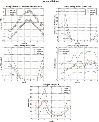
Figure 2. Seasonal variability of monthly averaged minimum and maximum air temperature, precipitation and snow cover at meteorological stations at Tarnow and Nowy Sacz, and runoff at gauging station in Koszyce Wielkie, with tenth and ninetieth percentiles of measured values. A comparison of hydro-climatic conditions at training, validation and testing periods.

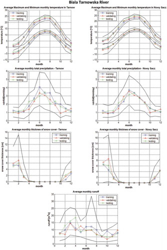
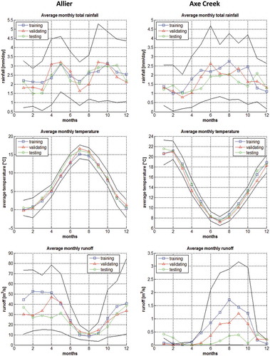
Figure 3. Seasonal variability of monthly averaged air temperature, precipitation and runoff, with tenth and ninety percentile of measured values at Allier and Axe Creek catchments. A comparison of hydro-climatic conditions at training, validation and testing periods.

Annapolis River catchment (546 km²) is located in the northern part of Nova Scotia, Canada. Its landscape in the middle part is generally flat, but in the north and south the steeper hills reach over 250 m a.s.l. Annapolis River is located within the Humid Continental Zone according to the Köppen Climate Classification. Snowfall occurs there from November to April but during winter months the significant variations in temperature may lead to frequent freezing and melting events. Peak rainfalls occur from September to November whilst in winter, snowfall prevails. Snow cover accumulates until February followed by the melting season in March. Most floods and large variability of runoff are noted during the November–April period. The concentration time of upper Annapolis catchment is slightly less than one day. The detailed, although not the most recent, description of the catchment may be found in Trescott (1968).

In this paper the 30 years of daily hydrological and meteorological measurements are used. The data are available from the Water Survey of Canada and Canada’s National Climate Data and Information Archive for the gauge station situated in Wilmot settlement and the meteorological station located at the Greenwood Airfield. Data collected during 30 years are divided into three sets of similar size: training set that includes data from 1980 to 1989, validation set, composed of data from 1990 to 1999, and finally the data collected during 2000–2009 period are left aside as the independent testing set. As may be noted from Fig. 1, the climatic and runoff conditions are similar for each dataset.

The data from Annapolis River catchment have already been used in some of our previous studies (Piotrowski and Napiorkowski 2011, 2012, 2013). As in the mentioned papers, in this paper at each kth day the one-lead-day discharge forecast Q(k + 1) for Wilmot is calculated based on the following hydro-meteorological measurements: the discharge, Q; maximum, UT, and minimum, LT, daily air temperatures; the total rainfall, RF; the total snowfall, SF; and the thickness of snow cover, SC. Based on the experience from previous studies, two various combinations of recently measured values collected during two recent days (k and k – 1) of hydro-meteorological variables are tested as MLP inputs in this paper. All considered variants of input nodes and the tested numbers of hidden nodes are defined in Table 1.

Table 1. Considered ANN architectures for each river. UT: maximum daily temperature (°C), LT: minimum daily temperature (°C), AT: average daily temperature (°C), ETP: daily potential evapotranspiration (mm), RF: daily rainfall excluding snowfall (mm), SF: daily snowfall (mm), PR: total daily precipitation (mm), SC: thickness of snow cover (cm), Q: river runoff (m³/s); k: the last recorded value of particular variable; k-1: the value of the variable recorded a day before; IN: number of input nodes (input variables), HN: number of hidden nodes, ON: number of output nodes; (N): data measured in Nowy Sacz; (T): data measured in Tarnow.

	Lp	ANN structure (IN, HN, ON)	Number of parameters	Input variables
Annapolis River	1	7-4-1	37	UTk, LTk, RFk, SFk, SCk; Qk; Qk-1
	2	7-5-1	46
	3	7-7-1	64
	4	7-9-1	82
	5	10-4-1	49	UTk, LTk, RFk, RFk-1, SFk, SFk-1, SCk; SCk-1; Qk; Qk-1
	6	10-5-1	61
	7	10-7-1	85
	8	10-9-1	109
Biala Tarnowska River	9	8-4-1	41	UT(N)k, LT(N)k, PR(N)k, PR(N)k-1, SC(N)k, SC(N)k-1, Qk, Qk-1
	10	8-5-1	51
	11	8-7-1	71
	12	8-9-1	91
	13	8-4-1	41	UT(T)k, LT(T)k, PR(T)k, PR(T)k-1, SC(T)k, SC(T)k-1, Qk, Qk-1
	14	8-5-1	51
	15	8-7-1	71
	16	8-9-1	91
	17	10-4-1	49	UT(N)k, UT(N)k-1, LT(N)k, LT(N)k-1, PR(N)k, PR(N)k-1, SC(N)k, SC(N)k-1, Qk, Qk-1
	18	10-5-1	61
	19	10-7-1	85
	20	10-9-1	109
	21	10-4-1	49	UT(T)k, UT(T)k-1, LT(T)k, LT(T)k-1, PR(T)k, PR(T)k-1, SC(T)k, SC(T)k-1, Qk, Qk-1
	22	10-5-1	61
	23	10-7-1	85
	24	10-9-1	109
	25	10-4-1	49	UT(N)k, UT(T)k, LT(N)k, LT(T)k, PR(N)k, PR(T)k, SC(N)k, SC(T)k, Qk, Qk-1
	26	10-5-1	61
	27	10-7-1	85
	28	10-9-1	109
	29	10-11-1	133
	30	14-4-1	65	UT(N)k, UT(T)k, LT(N)k, LT(T)k, PR(N)k, PR(N)k1, PR(T)k, PR(T)k-1, SC(N)k, SC(N)k-1, SC(T)k, SC(T)k-1, Qk, Qk-1
	31	14-5-1	81
	32	14-7-1	113
	33	14-9-1	145
Allier River	34	8-3-1a	31	ETPk, ETPk-1, PRk, PRk-1, PRk-2, PRk-3, Qk, Qk-1
	35	8-4-1a	41
	36	8-5-1a	51
	37	8-6-1a	61
	38	8-7-1a	71
	39	8-3-1b	31	ATk, ATk-1, PRk, PRk-1, PRk-2, PRk-3, Qk, Qk-1
	40	8-4-1b	41
	41	8-5-1b	51
	42	8-6-1b	61
	43	8-7-1b	71
	44	9-3-1	34	ETPk, ETPk-1, ATk, ATk-1, PRk, PRk-1, PRk-2, Qk, Qk-1
	45	9-4-1	45
	46	9-5-1	56
	47	9-6-1	67
	48	9-7-1	78
	49	10-3-1	37	ETPk, ETPk-1, ATk, ATk-1, PRk, PRk-1, PRk-2, PRk-3, Qk, Qk-1
	50	10-4-1	49
	51	10-5-1	61
	52	10-6-1	73
	53	10-7-1	85
	54	11-3-1	40	ETPk, ETPk-1, ATk, ATk-1, PRk, PRk-1, PRk-2, PRk-3, Qk, Qk-1, Qk-2
	55	11-4-1	53
	56	11-5-1	66
	57	11-6-1	79
	58	11-7-1	92
Axe Creek	59	8-4-1a	41	ETPk, ETPk-1, PRk, PRk-1, PRk-2, PRk-3, Qk, Qk-1
	60	8-5-1a	51
	61	8-6-1a	61
	62	8-7-1a	71
	63	8-4-1b	41	ATk, ATk-1, PRk, PRk-1, PRk-2, PRk-3, Qk, Qk-1
	64	8-5-1b	51
	65	8-6-1b	61
	66	8-7-1b	71
	67	9-4-1	45	ETPk, ETPk-1, ATk, ATk-1, PRk, PRk-1, PRk-2, Qk, Qk-1
	68	9-5-1	56
	69	9-6-1	67
	70	9-7-1	78
	71	10-4-1	49	ETPk, ETPk-1, ATk, ATk-1, PRk, PRk-1, PRk-2, PRk-3, Qk, Qk-1
	72	10-5-1	61
	73	10-6-1	73
	74	10-7-1	85
	75	11-4-1	53	ETPk, ETPk-1, ATk, ATk-1, PRk, PRk-1, PRk-2, PRk-3, Qk, Qk-1, Qk-2
	76	11-5-1	66
	77	11-6-1	79
	78	11-7-1	92

Biala Tarnowska River, a right-bank tributary of Dunajec River, is located in southern Poland in the Carpathian Mountains. The highest peaks within the catchment reach almost 1000 m a.s.l. and are located in the far south. In the north, closer to the city of Tarnow, hills are lower, reaching up to 550 m a.s.l. It is a typical mountainous river with slopes up to 8.6‰ in the upper part and about 0.9‰ in the lower part. Biala Tarnowska catchment area to the Koszyce Wielkie gauging station, which lies in the south-western suburbs of the city of Tarnow, equals 956.9 km². Like Annapolis catchment, Biala Tarnowska is located within the Humid Continental Zone according to the Köppen Climate Classification, and both catchments share similar climatic conditions during winter months. However, at Biala Tarnowska catchment, high levels of precipitation and large variation of runoff are observed during summer.

One-lead-day runoff forecasting Q(k + 1) in Koszyce Wielkie is performed based on hydro-meteorological measurements collected between 1970 and 2000. Like in the case of Annapolis River, the data are divided almost evenly into three sets. The data collected before 1 November 1980 compose the training set, the data collected between 1 November 1980 and 31 October 1990 are included in the validation set and the rest of the data form the testing set. The meteorological measurements used include: total daily precipitation, PR (rainfall and snowfall); thickness of snow cover, SC; and the daily minimum, LT, and maximum, UT, air temperature. The data are collected at two meteorological stations in the cities of Tarnow (T) and Nowy Sacz (N). The daily runoff, Q, is measured at Koszyce Wielkie gauging station. As this is, to the best of our knowledge, the first study aiming at runoff modelling by means of ANNs at Biala Tarnowska catchment, a number of cases with different input variables and numbers of hidden nodes is tested (see all considered variants in Table 1). In some tested variants the meteorological data from only one location, Tarnow or Nowy Sacz, are used.

Allier River flows through a mountainous part of south-central France, in the Massif Central (the highest peaks slightly exceeds 1500 m a.s.l.) within mainly mild Oceanic Climate. The catchment area up to Veille-Brioude, where the runoff is measured, equals 2269 km². The rainfalls are noted during the whole year, and in winter snow is not uncommon at higher elevations. Highest runoffs are observed in late spring and in autumn. A more detailed description of the catchment may be found in Thirel et al. (2015).

The available Allier catchment data (see also Vidal et al. 2010) include the runoff Q; precipitation PR; potential evapotranspiration PET; and mean air temperature T at the daily time scale for the 1 August 1958–31 July 2008 period. For the purpose of this study the data were divided into training (01 August 1958–31 December 1980), validation (1 January 1981–31 December 1995) and independent testing (1 January 1996–31 July 2008) sets. The tested variants of input variables used for daily runoff modelling Q(k + 1) are summarized in Table 1.

Axe Creek catchment up to Longlea (Victoria, Australia), where the runoff is measured, is smaller than the previously described ones (137 km²) and located in a relatively dry area, which, however, is also classified within Oceanic Climate according to the Köppen Climate Classification. The catchment is hilly (altitudes vary from 175 m to over 700 m a.s.l.) and mainly used for agriculture and pastures. Rainfall prevails during winter and spring months (snowfall is very uncommon), and runoff is observed mainly in this period; the rest of the year is often dry. The data for this catchment are non-stationary, as after 1997 the rainfall and runoff diminished noticeably in the whole region, what is known as the millennium drought (Potter and Chiew 2011, van Dijk et al. 2013). The non-stationarity is also clearly visible in Fig. 3. However, since 2009 the area is recovering and has become more wet again. A more detailed description of the catchment may also be found in Thirel et al. (2015) and Osuch et al. (2015).

For the 1973–2011 period the available daily measurements include runoff, Q (at Longlea); mean air temperature, T; potential evapotranspiration, PET; and precipitation, PR. The data measured before 1991 are included in the training set, the data from 1991–2000 period compose the validation set, and the most recent measurements are included in the independent testing set. As the data for this station are non-stationary and the runoff modelling is a real challenge, Axe Creek catchment gives a chance to evaluate the importance of ANN training and aggregation methods for daily Q(k + 1) runoff forecasting when climate change takes place.

All ANN architectures considered for each river are given in Table 1. For all rivers each ANN architecture is trained 50 times by means of LM algorithm, and the architecture that achieves the best performance is selected to be used for the further part of the study (comparison among training algorithms and evaluation of the importance of training and ensemble aggregation methods).

3 Multi-layer perceptron neural networks

The multi-layer perceptron ANN (Haykin 1999) consists of nodes grouped into input, hidden and output layers. A single hidden layer is considered enough to approximate continuous differentiable functions (Hornik et al. 1989), but there is no widely accepted rule regarding the number of hidden nodes (Zhang et al. 1998). The MLP neural network is defined as:

(1)

where y^p is a predicted value of the output variable, z_k, k = 1, …, K represents input variables, w and v are MLP weights to be optimized, J is the number of hidden units and f is the so-called activation function. As suggested in Shamseldin et al. (2002), who compared various activation functions for nodes in the hidden layer when ANN is used for flow forecasting, in the present paper the logistic activation function is used:

(2)

As the objective function the mean square error (MSE), required by LM algorithm, is chosen

(3)

where y is the measured value of the output variable and N is the number of observations. In the present study the input and output variables are normalized to [0,1] interval.

To prevent ANN overfitting to data (Haykin 1999), the early stopping approach in the variant proposed by Prechlet (1998) is used, even though Amari et al. (1997) showed that when the number of data exceeds the number of ANN parameters 30 times—as is the case in our study—the importance of using methods aiming to prevent overfitting is low. Early stopping requires the data to be divided into three parts: training (TR), validation (V) and independent testing (TE). When classical gradient-based methods are used to train ANNs, the derivatives of the objective function are estimated based on the training data only. If the error computed for training data diminishes, but the error evaluated for validation data increases, it is considered as a sign of overfitting. Training terminates after a predefined number of function calls or when the validation error exceeds its previously noted minimum value by 20% (as in Piotrowski and Napiorkowski 2013). In the case of LM algorithm no improvement is observed after 1000 function calls, hence this value is set as the maximum number of function calls. After termination, the best solution is chosen according to the performance for validation data.

Global optimization methods are usually stopped when the total number of objective function evaluations is reached, that is set to 10000D in this study, where D is the dimensionality of the problem (specified by the number of parameters to be optimized—in the case of ANNs, the number of weights w and v). As it is well known that metaheuristics cannot compete with gradient-based algorithms in terms of speed (Mandischer 2002, Ilonen et al. 2003), the maximum number of function calls used by metaheuristics is much larger than that used by LM algorithm. During the whole optimization process only the training data are used to guide the search by the metaheuristics. However, the best solution according to the validation set is remembered like in the case of gradient-based algorithms. When training terminates, such solution with the lowest objective function value for validation data is chosen as the best one found by the algorithm.

4 Tested metaheuristics

Metaheuristics, especially evolutionary algorithms or swarm intelligence methods (see, for example, the review in Boussaid et al. 2013), have become extremely popular in various applications. Due to the influx of novel optimization metaheuristics, their unavoidably subjective selection is necessary. In this paper the main attention is put on DE methods (Storn and Price 1995) that, although suffer from stagnation (Piotrowski 2014), are widely applied to ANN training in the literature. However, a number of other approaches are tested as well. The performance of ANNs trained by various metaheuristics is compared with the performance of ANNs optimized by LM algorithm. The initial values of MLP weights are randomly sampled within [–1,1] interval by almost all methods—the exceptions are SP-UCI (Chu et al. 2011) for which initial values are sampled within [–10,10] interval (because the expansion of simplexes is more rare than their contraction), and methods based on covariance matrix adaptation evolution strategy (CMA-ES), where initial solutions are generated from multi-dimensional normal distribution (see Hansen and Ostermeier 1996). Following the experience from Piotrowski and Napiorkowski (2011), the ANN weights are bounded within [–1000,1000] interval. Almost all algorithms are used with parameters suggested by their inventors; the details of some exceptions are given below. The following optimization methods were chosen for comparison (Differential Evolution is abbreviated as DE):

1. LM [Levenberg-Marquardt algorithm] gradient-based approach (Hagan and Menhaj 1994);

2. DEGL [DE with neighbourhood-based mutation operator] algorithm (Das et al. 2009), which uses Global and Local neighborhood-based mutation operation concept;

3. DE-SG [DE with separated groups] (Piotrowski et al. 2012a, 2012b), a variant of distributed DE methods, which is an updated version of grouped differential evolution algorithm (Piotrowski and Napiorkowski 2010); to speed up convergence, the parameter PNI is reduced to 10 and the parameter that defines migration probability MigProb is set to 1/PNI;

4. JADE [no full name is given in the source paper] (Zhang and Sanderson 2009), DE variant which introduces a novel mutation strategy and uses an external archive to remember some of the relatively “good” solutions that are lost during selection;

5. SADE [self-adaptive DE] (Qin et al. 2009), a classical adaptive DE variant;

6. SspDE [DE with self-adapting strategy and control parameters] (Pan et al. 2011), another variant of self-adaptive DE;

7. SFMDE [super-fit memetic DE] (Caponio et al. 2009), memetic approach that merges modified DE scheme with Nelder-Mead (1965) and Rosenbrock (1960) local search algorithms;

8. AM-DEGL [adaptive memetic DE with neighbourhood-based mutation operator] (Piotrowski 2013), another adaptive memetic DE approach;

9. DEahcSPX [DE with adaptive crossover-based local search] (Noman and Iba 2008), one of the earliest memetic DE variants;

10. MDE_pBX [modified DE with p-best crossover] (Islam et al. 2012), self-adaptive DE variant that introduces a novel mutation strategy;

11. CoDE [composite DE] (Wang et al. 2011), an algorithm which creates three offspring for each individual, the available mutation strategies and control parameters are solely based on the best performing solutions found in the literature;

12. DECLS [DE with chaotic local search and parameter adaptation] (Jia et al. 2011), memetic DE variant based on the chaotic local search mechanism;

13. CDE [clustering-based DE] (Cai et al. 2011), DE variant based on the concept of clustering;

14. AdapSS-JADE [adaptive strategy selection JADE] (Gong et al. 2011), another adaptive DE variant, based on JADE algorithm;

15. DCMA-ES [differential covariance matrix adaptation evolutionary algorithm] (Ghosh et al. 2012), the hybrid approach based on the CMA-ES (Hansen and Ostermeier 1996) and the basic DE, the population size is set to 5D;

16. CLPSO-DEGL [comprehensive learning particle swarm optimizer and DE with neighbourhood-based mutation operator hybrid algorithm] (Epitropakis et al. 2012), a hybrid algorithm merging the very popular PSO variant called CLPSO (Liang et al. 2006) with DEGL approach (Das et al. 2009), the initial velocities of particles are generated within [–20,+20] interval, the population size equals 40;

17. SP-UCI [shuffled complex evolution with principal components analysis–University of California at Irvine] (Chu et al. 2011), the improved version of SCE-UA method, it evolves four Nelder-Mead (Nelder and Mead 1965) based simplexes working together;

18. AMALGAM [a multi-algorithm genetically adaptive method for single objective optimization] (Vrugt et al. 2009), powerful multi-algorithm that distributes the search process into a few different metaheuristics, adaptively allocates the fitness function evaluation budget to each method and defines the rules of information exchange between them.

In our previous studies that, however, are not always related to runoff forecasting (Piotrowski et al. 2014, Piotrowski 2014), we found that, in the case of DE algorithms, the population size may have significant impact on the performance of ANN training. Hence, in this paper we test three population size settings for all non-hybrid DE variants used (numbered 2–14 in the list above), namely 1D, 3D and 5D (when D is the dimensionality of the problem), that are frequently used in DE literature (see Gamperle et al. 2002 and a brief discussion in Piotrowski 2013). This allows a more detailed insight into the relation between this DE control parameter and the achieved ANN performance.

5 Comparison of training methods

The selection of MLP architecture which is to be applied in further research is based on MSE values obtained when LM algorithm is used. Fifty runs of LM algorithm are performed for each variant of MLP architecture as given in Table 1. The 50-run mean and median MSE values achieved for testing data are illustrated in Fig. 4. Detailed results, namely mean, median, standard deviation and the best MSE achieved during 50-runs of LM algorithm for training, validation and testing datasets separately are reported in Supplementary Material, Table S1. In addition, the performances of naïve prediction (which consider today’s runoff as the forecast for tomorrow) and linear regression are given.

Figure 4. The 50-run mean and median MSE for testing data, achieved by different MLP architectures trained by LM algorithm. For comparison, the MSE of naïve prediction and linear regression (with inputs similar to the ones used in ANN architecture chosen for further tests) are shown. The symbols a and b in the case of Allier River and Axe Creek, and N and T in the case of Biala Tarnowska River refer to ANN versions defined in Table 1. For more detailed results see Supplementary Table 1 (available as supplementary material in the electronic version of the paper).

According to Fig. 4 and Supplementary Material, Table S1, the choice of the best MLP architecture for Annapolis River is not an easy task. Obviously, most important are the results obtained for the independent testing data, hence the choice should depend on them. One may see clear differences in the comparison of the mean and median results: the mean performance obtained by 7–9-1 architecture is marginally better than the mean performance achieved with 10–5-1 architecture, but the median performance for 10–5-1 architecture is much lower than that for the 7–9-1 one. Also, the best MSE among solutions obtained during 50-runs is lower in the case of 10–5-1 than 7–9-1 architecture. In addition, 10–5-1 architecture has fewer parameters (61) than the 7–9-1 one (82), hence the MLP with 10 inputs, 5 hidden nodes and a single output is selected for the comparison of different training methods on Annapolis catchment data. However, this 10–5-1 MLP architecture differs from the simpler 7–5-1 that was chosen as the best one in the previous studies (Piotrowski and Napiorkowski 2011, 2012). This is not surprising, as the division of data into training, validation and testing sets is different in the present study. Nonetheless, to show how much the performance of ensemble aggregation approach and particular optimization method depend on the number of MLP parameters, the results for the simpler 7–5-1 architecture with 46 parameters are also reported in this study.

In the case of Biala Tarnowska catchment the choice is much simpler. According to the testing data, both 50-run mean and median values are lowest for 10–9-1 architecture which includes meteorological measurements from both Tarnow and Nowy Sacz. The best architecture for Biala Tarnowska River requires 109 parameters to be optimized, that may pose additional difficulty to metaheuristics which are often affected by the curse of dimensionality.

Contrary to Annapolis or Biala Tarnowska, in the case of Allier and Axe Creek catchments the snow plays little or no role in runoff generation, and the information on daily maximum or minimum air temperatures is not available. Hence the main difficulty lies in verifying whether using both information on T and PET is necessary, and choosing the optimum number of recent Q, T, PET and PR measurements to be used as ANN inputs. From Fig. 4 and Supplementary Material, Table S1, one may find that for both catchments neither T nor PET should be omitted.

In the case of Allier River, the best mean and median results for testing data were achieved with 11–4-1 architecture that has 53 parameters; hence, this one is chosen for further research. However, a cautious reader may easily find that some simpler ANN architectures (8–4-1 b or 9–5-1) led to only slightly poorer results.

The choice of ANN architecture for Axe Creek is a bit more disputable—the results achieved with 9–5-1 and 9–7-1 architectures are very similar (9–6-1 turned out marginally poorer, probably by chance). Hence, again the simpler of the two (9–5-1, with 56 parameters) is chosen for further tests.

The comparison between the naïve model and the median results achieved by ANNs for all catchments shows that the MSE of the naïve model is at least about two times higher than the median MSE obtained from the best chosen ANN architecture. For Allier, Annapolis and Biala Tarnowska catchments the differences are even larger. The differences between ANNs and linear regression are obviously smaller, but still noticeable: for the testing data MSE obtained from the linear regression model is 1.4 to 1.56 times higher than the median MSE of the best ANN architecture for all catchments but Axe Creek, for which this relation equals 1.27.

The 50-run mean and median MSE values for testing data obtained by MLPs trained by all considered algorithms are shown in Fig. 5. Again, the more detailed results, namely the respective mean, median, best and standard deviation of MSE values obtained for all datasets are reported in Supplementary Material, Table S2. Wilcoxon two-sided rank-sum-test (Wilcoxon 1945) is used to assess the statistical significance of the differences between results achieved by various algorithms at 5% significance level (see Table 2). When we slightly informally refer to “statistically better” or “statistically poorer” algorithms in the discussion below, we understand that the difference between the results achieved by two algorithms is statistically significant at 5% significance level, and we call “better” the algorithm with lower mean square error; the other one is called “worse”. The number of algorithms from which a particular method is “worse” or “better” for every catchment is given in Table 2.

Figure 5. The 50-run mean and median MSE for testing data, achieved by selected MLP architectures trained by all tested algorithms. For more detailed results see Supplementary Table 2 (available as supplementary material in the electronic version of the paper). (Continued).

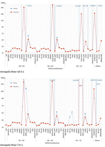
Figure 5. (Continued).

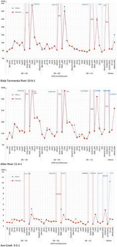
Table 2. Statistical significance of the results achieved by neural networks trained by different algorithms for each considered river, based on Wilcoxon rank-sum-test at the 5% significance level. In each row one finds the number of training variants from which the particular algorithm is better, worse, or the differences are not statistically significant.

		Annapolis 10-5-1			Annapolis 7-5-1
	Algorithm	better	similar	worse	better	similar	worse
	LM	30	9	5	27	12	5
DE – 5D	AM-DEGL	41	3	0	41	3	0
	DEGL	32	8	4	37	7	0
	DE-SG	11	6	27	8	5	31
	JADE	9	3	32	9	4	31
	SADE	17	5	22	16	8	20
	SspDE	12	5	27	12	7	25
	SFMDE	24	8	12	24	10	10
	DEahcSPX	0	4	40	1	3	40
	MDE_pBX	32	10	2	29	11	4
	CoDE	4	3	37	4	3	37
	DECLS	8	2	34	8	3	33
	CDE	12	5	27	9	8	27
	AdapSS-JADE	10	4	30	8	6	30
DE – 3D	AM-DEGL	41	3	0	37	6	1
	DEGL	32	9	3	30	13	1
	DE-SG	16	6	22	13	7	24
	JADE	12	7	25	12	8	24
	SADE	22	2	20	19	5	20
	SspDE	17	5	22	18	5	21
	SFMDE	25	7	12	23	8	13
	DEahcSPX	0	2	42	1	3	40
	MDE_pBX	32	9	3	27	13	4
	CoDE	4	4	36	4	4	36
	DECLS	8	3	33	11	7	26
	CDE	16	6	22	12	7	25
	AdapSS-JADE	11	6	27	14	7	23
DE – 1D	AM-DEGL	36	6	2	37	7	0
	DEGL	38	6	0	28	12	4
	DE-SG	32	8	4	28	11	5
	JADE	23	3	18	23	5	16
	SADE	25	8	11	29	11	4
	SspDE	25	9	10	29	11	4
	SFMDE	25	7	12	23	6	15
	DEahcSPX	1	3	40	0	1	43
	MDE_pBX	29	10	5	30	13	1
	CoDE	5	3	36	5	3	36
	DECLS	17	5	22	19	4	21
	CDE	25	7	12	27	10	7
	AdapSS-JADE	22	3	19	23	6	15
Others	DCMA-ES	1	3	40	1	3	40
	CLPSO-DEGL	34	8	2	32	11	1
	SP-UCI	25	9	10	21	9	14
	AMALGAM	4	4	36	4	4	36
		Biala Tarnowska			Allier			Axe
	Algorithm	better	similar	worse	better	similar	worse	better	similar	worse
	LM	38	6	0	41	3	0	24	15	5
DE – 5D	AM-DEGL	21	17	6	26	9	9	20	19	5
	DEGL	21	13	10	36	7	1	20	19	5
	DE-SG	8	4	32	10	4	30	9	5	30
	JADE	10	5	29	15	2	27	13	5	26
	SADE	15	6	23	19	14	11	18	10	16
	SspDE	9	5	30	20	11	13	12	6	26
	SFMDE	25	15	4	20	13	11	21	13	10
	DEahcSPX	0	4	40	0	4	40	0	3	41
	MDE_pBX	21	17	6	17	14	13	36	8	0
	CoDE	4	2	38	4	1	39	4	3	37
	DECLS	7	1	36	8	2	34	7	5	32
	CDE	13	5	26	8	2	34	7	5	32
	AdapSS-JADE	10	5	29	10	4	30	11	7	26
DE – 3D	AM-DEGL	21	17	6	31	5	8	20	18	6
	DEGL	21	17	6	38	6	0	30	14	0
	DE-SG	11	5	28	16	15	13	12	6	26
	JADE	21	17	6	16	6	22	18	5	21
	SADE	21	14	9	29	8	7	21	17	6
	SspDE	16	5	23	34	6	4	19	12	13
	SFMDE	25	15	4	20	12	12	20	12	12
	DEahcSPX	0	4	40	0	2	42	0	3	41
	MDE_pBX	21	14	9	20	11	13	26	13	5
	CoDE	4	2	38	5	1	38	4	3	37
	DECLS	8	3	33	10	4	30	7	8	29
	CDE	16	5	23	10	4	30	9	5	30
	AdapSS-JADE	16	5	23	14	1	29	18	3	23
DE – 1D	AM-DEGL	21	17	6	20	11	13	19	20	5
	DEGL	21	17	6	36	6	2	26	17	1
	DE-SG	34	8	2	36	5	3	26	13	5
	JADE	34	8	2	31	6	7	20	13	11
	SADE	38	5	1	37	6	1	36	8	0
	SspDE	40	4	0	39	5	0	38	6	0
	SFMDE	25	15	4	20	12	12	23	15	6
	DEahcSPX	0	4	40	1	3	40	0	3	41
	MDE_pBX	21	14	9	20	11	13	36	8	0
	CoDE	6	1	37	6	2	36	4	3	37
	DECLS	15	6	23	15	6	23	22	16	6
	CDE	41	3	0	32	4	8	26	16	2
	AdapSS-JADE	22	18	4	16	7	21	21	13	10
Others	DCMA-ES	0	4	40	1	3	40	3	1	40
	CLPSO-DEGL	21	17	6	20	12	12	37	7	0
	SP-UCI	21	17	6	16	6	22	7	10	27
	AMALGAM	8	8	28	6	2	36	7	11	26

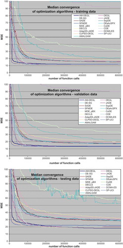
To verify the algorithm’s speed, the example of convergence plots of the median fitness of all applied metaheuristics used to train 10–5-1 MLP architecture for rainfall–runoff modelling at Annapolis River are shown in Fig. 6. As the fitness of the best individuals found so far according to the validation data are used to plot the convergence of different algorithms, such plots may be rugged for training and testing data. To avoid a blurry in Fig. 6, among DE variants, only results for those with NP = 5D are shown as this population size often led to the best results for Annapolis River runoff forecasting by means of MLPs.

Figure 6. Median convergence plots of all metaheuristics applied to ANN training with 10–5–1 architecture for runoff forecasting in Annapolis catchment (mean square errors for training, validation and testing data are plotted separately).

The comparison of the results obtained for testing data by ANNs trained with different algorithms may be summarized as follows:

1. Based on the data from four selected catchments, it is not possible to point out one metaheuristic that could be recommended to ANN training for runoff forecasting. Depending on the catchment, according to the results for the testing set, one could recommend the classical LM algorithm for Allier River, AM-DEGL for Annapolis River, CDE for Biala Tarnowska River (if mean performance is concerned) or SspDE for Axe Creek and possibly also Biala Tarnowska (if median performance is concerned, instead of mean).

2. A group of algorithms that do perform relatively well for each catchment include LM, DEGL, AM-DEGL (both with different, but preferably large population sizes), SADE and SspDE (both only with population size set to 1D). A few other methods (MDE_pBX, DE-SG, SFMDE, CDE, CLPSO-DEGL) perform well for most catchments, but in some runs achieve poorer results. The performance of SP-UCI is very uneven. To choose the best approach one may try to learn how many times the particular algorithm failed in comparison with other tested methods. For example, from Table 2 it may be noted that there are no algorithms statistically better than LM on Biala Tarnowska and Allier rivers, but when all five tested cases are considered, LM has been statistically worse than 15 other algorithms (five on each tested ANN architecture for Annapolis River, and five on Axe Creek data). Considering the results achieved for all catchments together, both AM-DEGL and DEGL with population 5D failed in comparison with 20 algorithms (mainly on Allier and Biala Tarnowska rivers), SADE with population 1D—with 17 algorithms (but almost only on tests performed on Annapolis River), SspDE with population size 1D—with 14 algorithms (only on Annapolis River), CLPSO-DEGL—with 21 algorithms (mainly on Allier and Biala Tarnowska). This shows that LM is among methods that most rarely perform significantly worse than other training algorithms. It may, however, also suggest that algorithms that overall perform best achieve some failures either on Annapolis, or on Biala Tarnowska and Allier River data. It seems that the search for the single best calibration method cannot be successful. At least five methods mentioned at the beginning of this paragraph should be regarded as similarly good for ANN training for runoff forecasting.

3. The choice of the best method usually does not depend on whether median or mean results are compared—the only exception is Biala Tarnowska River, but the differences between the performances of two algorithms that could be spotted as the best according to either median or mean is truly marginal. For the vast majority of algorithms, mean and median results are very similar and lead to akin rankings of algorithms. However, there are some exceptions—for a few among metaheuristics that perform poorly for ANN training (DEahcSPX, DCMA, AMALGAM, in some cases even CoDE) the mean performance for testing data is outstandingly higher than the median one, due to occasional very poor predictions achieved during some among 50 runs. This indicates poor generalization properties of the models calibrated with such algorithms.

4. The population size may have a large effect on the performance of many DE algorithms (especially SADE, SspDE, but also JADE, CDE, DE-SG), but low on some others (AM-DEGL, DEGL, MDE_pBX, SFMDE). DE variants that are very sensitive to the population size often perform best with their low values (1D). However, some well-performing methods, like DEGL or AM-DEGL, prefer higher population sizes (3D–5D). Some algorithms may require different population sizes for various catchments. Although this makes the general suggestion regarding the population size of DE algorithms used for ANN training difficult, the variants that perform better with larger population sizes (DEGL, AM-DEGL) are less sensitive to this control parameter than the algorithms that require lower population sizes (SADE, SspDE, DE-SG, CDE, JADE), hence the initial guess should be to start from small populations. If time allows, additional tests with larger ones are advised at the second step.

5. From Fig. 6 it is seen that there are large differences in training speed among various metaheuristics. Among the quickest are SFMDE and CLPSO-DEGL, but obviously, there are no metaheuristics that could compete with LM algorithm.

6. Some differences in the impact of snow on the prediction performance are noted for two catchments in which snowy conditions do regularly occur in winter (Annapolis and Biala Tarnowska). Considering only testing data for Annapolis catchment and the results achieved by the best performing algorithm in this case (AM-DEGL), the relative prediction error per day with snowfall or snow cover is 50% higher than that per snow-free day. In the case of Biala Tarnowska only the total sum of precipitation data are available (snowfall data are not provided separately), hence only days with snow cover could be considered. Taking into account only testing data and the best performing algorithm (although two algorithms perform almost evenly for this case, CDE with population size set to 1D is considered here), the relative prediction error per day with snow cover either in Tarnow or Nowy Sacz is 70% higher than that per snow-free day.

As LM is much quicker than metaheuristics, when differentiable objective function is used, there is little reason to apply metaheuristics to ANN training for runoff forecasting. If, however, due to any reason metaheuristics have to be used, a number of them, possibly with different population sizes, should be tested to choose the right one for the particular case.

6 Impact of ANN ensemble aggregation

The runoff forecasting performance may be improved by means of aggregation algorithms of ANN ensembles. A large number of methods aiming at the choice of ensemble members or aggregation of the results have already been proposed in the literature (see Breimann 1996, Granitto et al. 2005, Zheng 2009, Mendes-Moreira et al. 2012). In the present paper only two among the simplest methods are applied, in which all data from the training set are used by each ensemble member and aggregated forecasts y_n^P,agg are estimated either as a median of the forecasts (y_n^P,i) performed by all 50 MLP members (i = 1, …, 50), or as an average of the same forecasts. All 50 individuals are used as group members, because at least when the median rule is applied, the bigger the ensemble is, the better performance may be achieved (Zheng 2009). The median rules out the cases of occasional very poor predictions for particular time instances that may happen when ANN is applied to independent data that significantly differ from the training samples; however, the mean is more widely used in the literature. The same MLPs for which the statistics were reported in Fig. 5 and Supplementary Material, Table S2, are used as ensemble members. More precisely, the aggregated mean square error (MSEagg1) when the median is used is defined as

(4)

or, when mean is concerned (MSEagg2), as

(5)

where N is the number of data in the particular set. All 50 ensemble members are the outputs from ANNs trained by the same optimization algorithm and with the same MLP architecture. For a more detailed description of the method the reader is referred to Piotrowski et al. (2014) or DeWeber and Wagener (2014), where similar approaches were used for water temperature forecasting in rivers. The results obtained in the present study are provided in Table 3. The performances of both procedures may be summarized as follows:

1. For the testing data, the ensemble aggregated predictions by means of median (MSEagg1) are almost always lower than the 50-run median or mean of MSE of individual models. This is observed for all catchments and all algorithms. However, the difference between median performance of single models and the performance of aggregated ensemble may significantly depend on the training algorithm. For example, in the case of Biala Tarnowska River when ANNs are trained by AM-DEGL with population size set to 1D, the median MSE equals almost 83.7 (see Fig. 5 and Supplementary Material, Table S2), but the MSEagg1 is 15% lower. For the same catchment the respective values achieved by ANNs trained by DEahcSPX are 289.183 and 289.152, hence the improvement is truly marginal.

2. Aggregation using the mean from the ensemble (MSEagg2) in the vast majority of cases leads to slightly larger improvement. The results achieved by the best algorithms for a particular catchment are always better when the mean instead of the median is used as the aggregation method. With the exception of Axe Creek data, the differences between MSEagg1 and MSEagg2 are small when well-chosen training algorithms are considered. However, as very poor predictions are not ruled out when the mean is used, this method does not always eliminate pitfalls noted occasionally by some algorithms that perform poorly for ANN training.

3. In the case of Annapolis River the best MSEagg1 and MSEagg2 values for testing data are found when 10–5-1 MLP are trained by AM-DEGL algorithm with population size set to 3D. They are lower by about 10% than the 50-run mean or median MSE of individual models trained by the same algorithm. When aggregated results achieved by 7–5-1 MLP architecture are considered, AM-DEGL (with population size 1D) or MDE_pBX (with population size 5D) perform best, depending on whether the median or the mean is used as the aggregation method. In the case of Biala Tarnowska River, the lowest MSEagg is obtained by CDE (with population size 1D). For Allier River SFMDE (again with population size 1D) leads to the best aggregated results, irrespective of the aggregation method. However, in the case of Axe Creek, the lowest MSEagg1 is achieved with MDE_pBX with population size 5D, but based on MSEagg2 SP-UCI would be called the best method. From Table 3 one may find that MSEagg1 and MSEagg2 achieved by ANNs trained by means of roughly the 10 best algorithms are relatively similar for most catchments (Axe Creek data are an exception). It should also be noted that frequently after ensemble aggregation, algorithms with population size settings different from the one that won for raw results (Fig. 5 and Supplementary Material, Table S2) perform best. Hence, when ensemble aggregated results are compared, one may divide ANN training methods into two parts: a large group of algorithms that cannot be recommended for that task, and another large group of methods that perform, roughly speaking, similarly well. In other words, aggregation of ANN ensembles increases the number of training methods that show acceptable performance.

Table 3. The performance of aggregated MLP ensembles composed of 50 members (MSEagg1 and MSEagg2, see equations 4 and 5) trained with different methods. The best results obtained for each river are bolded.

			MEDIAN			MEAN
		algorithm	TR	V	TE	TR	V	TE
		LM	10.571	12.765	19.058	10.252	12.563	18.908
Annapolis River 10-5-1	DE – 5D	AM-DEGL	11.200	12.746	17.135	11.114	12.726	17.345
		DEGL	10.576	12.528	18.676	10.279	12.377	18.341
		DE-SG	14.406	16.380	28.085	14.342	16.318	27.829
		JADE	14.775	16.665	28.480	14.600	16.440	27.934
		SADE	13.624	15.345	26.065	13.053	14.661	24.574
		SspDE	14.439	16.311	26.841	14.347	16.149	26.529
		SFMDE	11.719	13.106	20.824	11.654	13.119	20.875
		DEahcSPX	62.867	66.380	101.278	60.325	62.036	1775.446
		MDE_pBX	10.642	12.370	18.297	10.211	12.158	17.902
		CoDE	20.047	21.019	41.585	19.299	20.140	41.283
		DECLS	15.143	16.951	28.074	14.890	16.555	27.182
		CDE	14.061	15.486	27.627	13.965	15.260	27.019
		AdapSS-JADE	14.843	16.506	28.463	14.668	16.297	28.107
	DE – 3D	AM-DEGL	10.865	12.774	17.129	10.706	12.644	16.987
		DEGL	10.371	12.390	18.034	9.777	12.131	17.277
		DE-SG	14.065	15.638	27.138	13.835	15.455	26.675
		JADE	14.279	15.965	27.755	13.979	15.712	27.262
		SADE	12.761	14.451	24.639	12.451	13.944	23.278
		SspDE	13.902	15.647	26.578	13.629	15.248	25.740
		SFMDE	11.398	12.860	20.417	11.240	12.820	20.233
		DEahcSPX	72.268	77.592	117.270	624.566	72.219	23.859.9
		MDE_pBX	10.411	12.326	18.480	9.769	12.013	17.521
		CoDE	19.336	20.484	40.923	18.872	19.879	38.790
		DECLS	14.775	16.466	27.298	14.537	16.169	26.597
		CDE	13.716	14.824	26.621	13.603	14.650	25.900
		AdapSS-JADE	14.256	15.711	27.242	14.171	15.550	26.707
	DE – 1D	AM-DEGL	10.833	12.435	17.984	10.629	12.340	17.541
		DEGL	10.215	12.409	17.515	9.916	12.238	17.099
		DE-SG	10.976	12.892	19.113	10.791	12.726	18.990
		JADE	12.423	14.021	22.109	11.893	13.597	20.754
		SADE	11.154	13.003	19.983	11.140	13.007	20.167
		SspDE	11.273	13.108	20.160	11.197	13.050	20.100
		SFMDE	11.741	13.067	20.950	11.582	13.001	20.449
		DEahcSPX	52.155	56.717	96.999	72030.850	52.371	103936.700
		MDE_pBX	10.594	12.550	19.014	10.116	12.320	18.813
		CoDE	17.387	18.058	37.707	2855.166	17.232	5651.197
		DECLS	12.798	14.207	23.861	12.725	14.064	23.117
		CDE	10.983	12.821	21.615	10.824	12.736	21.135
		AdapSS-JADE	12.623	13.999	23.096	12.060	13.589	21.740
	Others	DCMA-ES	44.546	46.550	75.687	42.532	43.959	35266.100
		CLPSO-DEGL	10.518	12.420	18.427	10.038	12.273	17.717
		SP-UCI	10.800	12.486	18.467	300.733	12.348	633.811
		AMALGAM	13.857	15.605	29.281	14.232	15.905	79244.400
Annapolis River 7-5-1		LM	10.471	12.871	18.688	9.704	12.416	18.354
	DE – 5D	AM-DEGL	11.555	13.037	18.039	11.485	13.017	17.975
		DEGL	10.875	12.868	17.864	10.169	12.393	17.197
		DE-SG	14.592	16.208	27.422	14.488	16.062	26.877
		JADE	14.204	15.932	26.905	13.956	15.697	26.203
		SADE	13.894	15.680	26.094	13.692	15.246	25.175
		SspDE	14.077	15.987	26.223	13.985	15.756	25.819
		SFMDE	12.096	13.203	20.901	11.982	13.144	20.854
		DEahcSPX	58.078	61.692	90.839	52.696	56.265	80.441
		MDE_pBX	10.799	12.702	18.667	10.114	12.326	17.117
		CoDE	16.896	18.167	35.758	16.229	17.461	33.126
		DECLS	14.695	16.388	26.852	14.646	16.251	26.606
		CDE	13.941	15.183	26.675	13.898	15.095	26.502
		AdapSS-JADE	14.333	15.858	27.139	14.155	15.612	26.144
	DE – 3D	AM-DEGL	11.225	13.002	17.866	11.044	12.916	17.781
		DEGL	10.452	12.670	18.610	9.679	12.205	17.592
		DE-SG	13.995	15.494	25.710	13.821	15.253	24.997
		JADE	13.925	15.639	26.552	13.743	15.385	25.663
		SADE	13.090	14.669	23.799	12.707	14.137	22.890
		SspDE	13.445	15.021	23.867	13.293	14.816	23.378
		SFMDE	12.260	13.249	21.156	12.139	13.163	20.722
		DEahcSPX	57.464	61.802	91.271	52.983	57.557	3464.599
		MDE_pBX	10.413	12.601	18.407	9.565	12.131	17.588
		CoDE	17.230	18.450	34.912	16.521	17.757	31.078
		DECLS	14.200	15.634	24.761	14.003	15.397	24.255
		CDE	13.594	14.484	26.281	13.540	14.324	24.959
		AdapSS-JADE	13.603	15.000	25.120	13.194	14.623	23.855
	DE – 1D	AM-DEGL	11.191	12.913	17.588	10.878	12.758	17.459
		DEGL	9.211	12.196	18.417	8.972	12.011	17.578
		DE-SG	11.131	13.116	19.743	10.797	12.843	20.488
		JADE	12.302	13.931	21.471	11.548	13.328	18.971
		SADE	11.445	13.182	19.822	11.320	13.088	19.533
		SspDE	11.571	13.306	19.684	11.431	13.166	19.575
		SFMDE	12.270	13.210	21.487	12.186	13.151	21.107
		DEahcSPX	15.078	16.824	31.354	39408.140	23.006	53347.760
		MDE_pBX	10.968	12.861	19.068	10.420	12.502	18.615
		CoDE	15.642	16.616	29.798	15.151	16.257	27.303
		DECLS	13.023	14.160	23.336	12.911	14.032	22.783
		CDE	11.168	13.020	20.880	11.033	12.883	20.376
		AdapSS-JADE	12.061	13.429	21.949	10.986	12.879	20.075
	Others	DCMA-ES	39.712	43.625	72.011	1634.280	40.740	4177.563
		CLPSO-DEGL	10.731	12.641	18.261	10.529	12.397	17.961
		SP-UCI	11.074	12.932	18.642	10.350	12.550	59.602
		AMALGAM	13.134	14.611	25.955	23.290	14.323	25800.370
Biala Tarnowska River 10-9-1		LM	55.184	51.193	72.517	54.693	51.044	71.862
	DE – 5D	AM-DEGL	64.438	42.280	75.061	63.770	41.982	75.090
		DEGL	63.820	41.050	78.011	63.334	41.073	78.136
		DE-SG	93.962	63.871	93.171	93.042	61.359	92.150
		JADE	92.207	60.612	90.703	90.862	59.130	88.941
		SADE	83.802	54.405	83.902	79.008	50.803	81.692
		SspDE	93.464	63.648	91.057	91.916	61.305	91.249
		SFMDE	59.573	45.188	71.427	59.069	44.951	71.133
		DEahcSPX	236.267	148.267	283.641	47973.610	122.565	30174.920
		MDE_pBX	63.761	41.927	76.518	59.810	40.751	73.625
		CoDE	154.146	84.031	164.428	144.857	77.539	153.725
		DECLS	95.531	58.747	97.628	96.292	58.466	98.195
		CDE	88.304	51.457	82.587	86.736	49.972	81.883
		AdapSS-JADE	90.771	56.976	89.056	89.859	55.432	88.768
	DE – 3D	AM-DEGL	59.805	42.213	74.070	60.856	42.500	74.202
		DEGL	61.866	41.533	76.684	61.017	41.470	75.227
		DE-SG	87.369	57.823	85.743	85.703	55.078	84.748
		JADE	61.866	41.533	76.684	61.017	41.370	75.227
		SADE	76.138	47.165	77.776	74.243	46.730	76.626
		SspDE	81.178	52.145	83.719	80.519	50.894	83.260
		SFMDE	60.647	46.409	71.301	60.368	45.108	71.021
		DEahcSPX	247.716	153.210	289.101	33131.220	137.475	57495.830
		MDE_pBX	66.410	41.916	78.304	64.566	41.450	76.780
		CoDE	138.070	81.280	152.468	131.105	74.192	143.267
		DECLS	88.440	52.607	88.979	88.596	51.477	89.024
		CDE	80.730	47.222	79.153	81.475	46.419	79.065
		AdapSS-JADE	83.877	51.227	81.456	83.012	50.294	81.364
	DE – 1D	AM-DEGL	58.349	41.208	72.363	59.780	40.172	71.398
		DEGL	63.196	42.041	78.033	61.753	42.277	75.707
		DE-SG	71.906	48.561	72.308	70.827	47.432	72.192
		JADE	68.224	43.709	73.270	67.555	44.060	72.933
		SADE	66.081	43.210	70.970	64.490	42.796	71.480
		SspDE	66.482	42.152	71.539	65.426	42.518	71.593
		SFMDE	58.290	44.159	72.245	57.402	43.904	70.873
		DEahcSPX	273.373	174.899	289.152	839579.100	135.492	134.655.1
		MDE_pBX	60.962	42.520	76.249	59.310	41.990	77.139
		CoDE	107.595	58.909	126.778	102.941	57.051	117.888
		DECLS	77.481	42.507	82.763	76.009	42.283	81.835
		CDE	61.409	42.110	69.057	62.313	41.759	67.820
		AdapSS-JADE	67.780	43.348	73.279	64.989	42.102	100.600
	Others	DCMA-ES	247.881	168.308	281.190	207.220	142.721	231.280
		CLPSO-DEGL	56.184	42.486	74.557	55.487	42.891	73.592
		SP-UCI	65.995	42.294	77.089	61.936	40.846	73.447
		AMALGAM	69.227	48.369	83.754	67.378	44.270	83.499
Allier River 11-4-1		LM	135.990	108.040	69.740	134.060	104.570	69.820
	DE – 5D	AM-DEGL	143.930	98.570	72.140	142.560	97.170	70.180
		DEGL	133.370	94.750	72.420	131.850	92.140	72.760
		DE-SG	271.000	189.300	110.240	265.350	186.150	107.150
		JADE	273.350	190.380	112.510	264.770	184.380	106.430
		SADE	226.480	152.180	83.400	212.510	142.280	80.440
		SspDE	245.490	164.960	93.020	240.830	162.580	90.030
		SFMDE	182.000	118.950	67.020	182.030	117.240	66.780
		DEahcSPX	923.260	681.470	476.140	69225.170	568.080	65929.250
		MDE_pBX	134.370	93.330	67.280	133.540	90.990	66.720
		CoDE	350.850	234.110	165.800	330.600	219.450	147.220
		DECLS	268.840	183.150	103.090	265.740	176.840	99.060
		CDE	280.100	195.820	118.060	274.620	192.810	112.160
		AdapSS-JADE	277.940	194.390	113.390	270.310	186.830	108.330
	DE – 3D	AM-DEGL	145.680	99.190	71.050	142.640	97.550	68.310
		DEGL	139.290	98.850	72.540	137.930	96.240	72.200
		DE-SG	213.530	142.540	79.770	204.110	136.810	77.270
		JADE	257.000	179.870	102.130	252.550	174.230	98.550
		SADE	194.660	126.820	74.950	185.260	123.070	75.020
		SspDE	186.450	118.380	69.780	183.730	118.540	70.400
		SFMDE	188.120	120.750	75.510	186.150	119.960	71.470
		DEahcSPX	1190.520	879.940	648.980	117189.20	655.970	228949.300
		MDE_pBX	136.800	92.710	68.650	135.800	92.690	68.160
		CoDE	337.400	219.370	154.860	311.130	205.020	137.660
		DECLS	240.820	156.330	86.520	235.740	150.670	86.570
		CDE	267.750	186.880	111.230	259.490	179.970	104.200
		AdapSS-JADE	163.820	179.660	101.170	259.960	175.710	96.670
	DE – 1D	AM-DEGL	143.100	100.650	71.900	141.080	97.250	70.510
		DEGL	133.260	97.350	76.450	133.280	97.240	75.530
		DE-SG	134.070	105.440	75.050	133.130	104.780	75.730
		JADE	200.520	132.100	77.860	182.940	122.220	75.290
		SADE	145.880	106.640	73.870	145.810	107.230	74.320
		SspDE	147.900	105.850	73.530	146.220	105.950	73.690
		SFMDE	166.800	105.610	66.640	168.920	105.780	65.940
		DEahcSPX	478.240	342.900	288.860	1961478.000	292.050	1722295.000
		MDE_pBX	137.190	98.820	69.720	136.610	96.400	67.740
		CoDE	299.360	193.930	139.080	278.470	185.330	23572.980
		DECLS	196.960	124.970	76.430	195.010	122.920	74.820
		CDE	153.640	111.830	71.660	153.310	109.730	69.650
		AdapSS-JADE	220.230	146.090	82.670	202.370	131.660	76.950
	Others	DCMA-ES	744.570	529.900	362.190	686.970	485.900	201813.400
		CLPSO-DEGL	135.740	93.100	71.780	133.910	91.360	70.740
		SP-UCI	145.320	96.700	72.790	142.090	92.880	122.940
		AMALGAM	223.270	143.940	94.220	5516.800	136.850	52219.140
Axe DCreek 9-5-1		LM	2.290	1.264	2.222	2.306	1.270	2.142
	DE – 5D	AM-DEGL	2.940	1.425	2.104	2.908	1.396	1.973
		DEGL	2.186	1.277	2.010	2.193	1.275	1.986
		DE-SG	4.803	1.881	3.141	4.775	1.858	3.122
		JADE	4.693	1.805	2.998	4.673	1.797	2.981
		SADE	4.479	1.708	2.843	3.952	1.605	2.491
		SspDE	4.743	1.824	3.057	4.670	1.181	2.987
		SFMDE	3.601	1.413	2.648	3.363	1.367	2.477
		DEahcSPX	8.065	2.935	4.369	109756.100	2.556	117242.500
		MDE_pBX	2.234	1.286	1.867	2.238	1.274	1.837
		CoDE	5.670	1.954	3.804	5.575	1.925	3.279
		DECLS	4.939	1.860	3.223	4.873	1.856	3.162
		CDE	4.982	1.780	3.225	4.941	1.771	3.223
		AdapSS-JADE	4.819	1.763	3.054	4.791	1.750	3.043
	DE – 3D	AM-DEGL	2.556	1.299	2.094	2.609	1.291	1.891
		DEGL	2.171	1.306	1.967	2.183	1.307	1.911
		DE-SG	4.632	1.826	3.036	4.407	1.755	2.934
		JADE	4.474	1.700	2.828	4.374	1.675	2.780
		SADE	3.827	1.549	2.544	3.142	1.427	2.105
		SspDE	4.385	1.679	2.781	4.044	1.608	2.615
		SFMDE	3.673	1.438	2.635	3.457	1.398	2.561
		DEahcSPX	8.109	2.904	15.993	112116.800	2.673	331900.800
		MDE_pBX	2.183	1.284	2.209	2.267	1.274	2.010
		CoDE	5.685	1.934	3.772	9.128	1.911	314.204
		DECLS	4.757	1.772	3.050	4.605	1.765	2.971
		CDE	4.758	1.691	3.142	4.676	1.668	3.095
		AdapSS-JADE	4.540	1.653	2.903	4.445	1.629	2.857
	DE – 1D	AM-DEGL	2.403	1.233	1.901	2.422	1.243	1.757
		DEGL	2.140	1.328	1.922	2.136	1.309	2.050
		DE-SG	2.210	1.331	2.186	2.280	1.316	2.065
		JADE	4.109	1.591	2.726	3.694	1.510	2.416
		SADE	2.511	1.391	2.072	2.542	1.377	1.954
		SspDE	2.335	1.349	1.968	2.398	1.347	1.830
		SFMDE	3.587	1.386	2.538	3.451	1.367	2.406
		DEahcSPX	7.797	2.922	4.553	62178.330	2.394	145465.600
		MDE_pBX	2.209	1.368	1.930	2.247	1.345	1.808
		CoDE	5.543	1.876	3.806	683.593	1.817	687.517
		DECLS	4.076	1.565	2.619	3.731	1.509	2.339
		CDE	2.503	1.374	2.171	2.653	1.364	2.015
		AdapSS-JADE	4.189	1.553	2.681	3.757	1.467	2.378
	Others	DCMA-ES	8.085	3.019	4.802	750.279	2.594	896.037
		CLPSO-DEGL	2.296	1.309	1.944	2.324	1.284	1.850
		SP-UCI	2.199	1.225	2.219	2.198	1.198	1.729
		AMALGAM	4.140	1.559	2.548	3.652	1.524	16.664

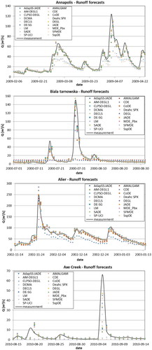
In Fig. 7 the aggregated runoff predictions for selected time periods at each considered catchment are illustrated. The aggregated predictions obtained by means of all training methods are shown, but among DE variants only those with selected population sizes (5D in the case of Annapolis River, 1D for other catchments) are chosen. For some days forecasts achieved from MLPs trained with almost any method are very similar, but in other cases large differences are clearly seen. Also the poor performance of some methods, like DEahcSPX, DCMA-ES and AMALGAM for ANN training may be visually observed.

Figure 7. Aggregated runoff predictions for selected hydrological situations from testing data for four considered catchments.

7 Conclusions

There are two main goals of this paper, namely comparing a number of metaheuristics with the Levenberg-Marquardt algorithm on ANN training for runoff forecasting at different catchments, and verifying the importance of the choice of ANN training method with the importance of very simple ensemble aggregation approaches.

In the present paper it is found that the performances of ANNs trained by different metaheuristics (hence the efficiency of a particular training method) significantly depend on the catchment. Data from four different catchments were used as the basis for the study, and none among several tested training algorithms perform best for more than a single catchment. Hence, based on this experiment, the choice of a single superior method is not possible. However, one may point out a group of metaheuristics that perform well for all (DEGL, AM-DEGL, SADE, SspDE) or most catchments (MDE_pBX, DE-SG, SFMDE, CDE, CLPSO-DEGL) and a similarly large group of methods that often fail to achieve reasonable performance when applied to ANN training for runoff forecasting. As the majority of population-based metaheuristics tested in this paper belong to the so-called Differential Evolution family of methods, the impact of the population size on the performance of such algorithms has also been verified. It was found that the majority of Differential Evolution methods perform best with low population size (especially SADE and SspDE). On the other hand, some well performing variants (especially AM-DEGL and DEGL) require rather higher population sizes.

Of main importance is that no metaheuristic may be said to outperform the classical Levenberg-Marquardt algorithm that turns out to be the best method for a single catchment (Allier River) and is ranked among the best performing optimization approaches for each catchment. As metaheuristics are always outstandingly slower than the Levenberg-Marquardt algorithm, when differentiable objective function is used it is difficult to suggest using any metaheuristic to ANN training for runoff forecasting. Some metaheuristics may probably perform better than the Levenberg-Marquardt algorithm for ANN training in a particular case, but significant effort is needed to find the proper one(s) for the specific catchment.

To verify how ensemble aggregation may improve the results obtained with the help of various training algorithms, all ensemble members were optimized by the same training method. It was found that the performance achieved by means of aggregation of ANN ensembles is much better than the mean or median performances of single models. Even the simplest methods of ensemble aggregation (by taking the mean or median from all predictions of ensemble members) turns out to be more important than the choice of the training method from among the well performing ones. However, if some metaheuristics from the group that perform poorly are used, the gain from ensemble aggregation would not be able to counterbalance the harm made by a poor optimizer. In this respect the proper choice of optimization method remains crucial.

The data observed at one among four tested catchments (Axe Creek) are not stationary, and a clear change in both climatic and runoff conditions (drying) has been observed at the beginning of this century. The experiment with runoff forecasting for such data by means of ANNs trained on measurements collected before the drought period lead to the results that could be expected—the forecasts were of rather poor quality. However, the performance of Axe Creek runoff forecasting varied significantly between ANNs trained with different optimization algorithms, and the use of ensemble aggregation approach turned out at least no less important than in the cases of the other catchments. It shows that, although the observed change in the hydro-climatic conditions clearly hamper forecasting quality, it does not root out the importance of the proper choice of training algorithms and application of ensemble aggregation approaches.

The results from this paper are, of course, limited, at least by the number of catchments tested or the specific metaheuristics used. As several methods were tested, it may be expected that the results do not depend on the choice of the specific one, but the possibility that the best existing approach was omitted, or that more attention should be paid to, for example, Particle Swarm Optimization or Genetic Algorithms, instead of Differential Evolution, cannot be ignored. The research also does not aim at ensemble modelling that could be suggested instead of ensemble aggregation (see Boucher et al. 2010), does not put attention on the catchments located in the arctic, high mountains or humid tropical climates and does not address the problem of ensemble size or ANN type used. All such issues could be considered for future studies.

The way the comparison is done may affect our findings. For example, recently an interesting idea to modify the approach to avoid overfitting by considering training and validation as two different criteria and using a multiobjective optimization metaheuristics has been proposed (Taormina and Chau 2015). It remains an open question if this could modify the conclusions from our study.

Finally, although it has been well known for years that all metaheuristics must perform equally well on all possible problems (Wolpert and Macready 1997), in some recent studies it was shown how fragile the comparison of metaheuristics may be even if it is based on only a few well defined problems. For example Derrac et al. (2014) noted that if, instead of the statistical significance of differences between the final results achieved by various metaheuristics, one would use statistical tests to verify the differences in the convergence properties of such methods, much different ranking of algorithms may be achieved. Piotrowski (2015) showed that very different rankings of algorithms may be achieved when one performs tests either by searching for the minimum or for the maximum of exactly the same functions, even if the bounds and number of allowed function calls are the same. Kononova et al. (2015) showed that in many optimization metaheuristics a structural bias may be observed, i.e. they are more prone to visit some parts of the search space. Sorensen (2015) seriously questioned the way the modern metaheuristics are motivated, and found that many of them are simply developed without a scientific rigour. The most unexpected may be, however, the result of the literature survey performed by Mernik et al. (2015), who studied all easily available publications on a metaheuristic called Artificial Bee Colony that were published until August 2013 and found that, depending on the evaluation criteria, between 40% and 67% of such studies led to probably not trustworthy results due to improperly made comparisons among different methods. This must be an additional warning for practitioners that would promote yet another metaheuristics as a method for ANN training, or any other goal.

Acknowledgements

This work was supported within statutory activities [no. 3841/E-41/S/2014] of the Ministry of Science and Higher Education of Poland.

Disclosure statement

No potential conflict of interest was reported by the authors.

References

- Abaza, M., et al., 2013. A comparison of the Canadian global and regional meteorological ensemble prediction systems for short-term hydrological forecasting. Monthly Weather Review, 141 (10), 3462–3476. doi:10.1175/MWR-D-12-00206.1
- Abbott, M.B., et al., 1986. An introduction to the European hydrological system – Système Hydrologique Europèen, SHE. 1 History and philosophy of a physically-based, distributed modelling system. Journal of Hydrology, 87, 61–77. doi:10.1016/0022-1694(86)90115-0
- Abrahart, R.J., et al., 2012a. Two decades of anarchy? Emerging themes and outstanding challenges for neural network river fore-casting. Progress in Physical Geography, 36 (4), 480–513. doi:10.1177/0309133312444943
- Abrahart, R.J., Mount, N.J., and Shamseldin, A.Y., 2012b. Neuroemulation: definition and key benefits for water resources research. Hydrological Sciences Journal, 57 (3), 407–423. doi:10.1080/02626667.2012.658401
- Adamowski, J. and Chan, H.F., 2011. A wavelet neural network conjunction model for groundwater level forecasting. Journal of Hydrology, 407 (1–4), 28–40. doi:10.1016/j.jhydrol.2011.06.013
- Adamowski, J. and Karapataki, C., 2010. Comparison of multivariate regression and artificial neural networks for peak urban water-demand forecasting: evaluation of different ANN learning algorithms. Journal of Hydrologic Engineering, 15, 729–743. doi:10.1061/(ASCE)HE.1943-5584.0000245
- Amari, S., et al., 1997. Asymptotic statistical theory of overtraining and cross-validation. IEEE Transactions on Neural Networks, 8 (5), 985–996. doi:10.1109/72.623200
- Bergström, S., 1976. Development and application of a conceptual runoff model for Scandinavian catchments. SMHI Report RHO 7, Norrköping, 134 pp.
- Boucher, M.A., Laliberte, J.P., and Anctil, F., 2010. An experiment on the evolution of an ensemble of neural networks for streamflow forecasting. Hydrology and Earth System Sciences, 14, 603–612. doi:10.5194/hess-14-603-2010
- Boucher, M.-A., Perreault, L., and Anctil, F., 2009. Tools for the assessment of hydrological ensemble forecasts obtained by neural networks. Journal of Hydroinformatics, 11 (3–4), 297–307. doi:10.2166/hydro.2009.037
- Boussaid, I., Lepagnot, J., and Siarry, P., 2013. A survey on optimization metaheuristics. Information Sciences, 237, 82–117. doi:10.1016/j.ins.2013.02.041
- Breiman, L., 1996. Bagging predictors. Machine Learning, 24 (2), 123–140. doi:10.1007/BF00058655
- Brochero, D., Anctil, F., and Gagné, C., 2011a. Simplifying a hydrological ensemble prediction system with a backward greedy selection of members - part 1: Optimization criteria. Hydrology and Earth System Sciences, 15, 3307–3325. doi:10.5194/hess-15-3307-2011
- Brochero, D., Anctil, F., and Gagné, C., 2011b. Simplifying a hydrological ensemble prediction system with a backward greedy selection of members - part 2: generalization in time and space. Hydrology and Earth System Sciences, 15, 3327–3341. doi:10.5194/hess-15-3327-2011
- Bullinaria, J.A. and AlYahya, K., 2014. Artificial bee colony training of neural networks: comparison with back-propagation. Memetic Computing, 6 (3), 171–182. doi:10.1007/s12293-014-0137-7
- Cai, Z.H., et al., 2011. A clustering-based differential evolution for global optimization. Applied Soft Computing, 11 (1), 1363–1379. doi:10.1016/j.asoc.2010.04.008
- Caponio, A., Neri, F., and Tirronen, V., 2009. Super-fit control adaptation in memetic differential evolution frameworks. Soft Computing, 13 (8–9), 811–831. doi:10.1007/s00500-008-0357-1
- Carcano, E.C., et al., 2008. Jordan recurrent neural network versus IHACRES in modelling daily streamflows. Journal of Hydrology, 362, 291–307. doi:10.1016/j.jhydrol.2008.08.026
- Chau, K.W., 2006. Particle swarm optimization training algorithm for ANNs in stage prediction of Shing Mun River. Journal of Hydrology, 329 (3–4), 363–367. doi:10.1016/j.jhydrol.2006.02.025
- Chu, W., Gao, X., and Sorooshian, S., 2011. A new evolutionary search strategy for global optimization of high-dimensional problems. Information Sciences, 181 (22), 4909–4927. doi:10.1016/j.ins.2011.06.024
- Cloke, H.L. and Pappenberger, F., 2009. Ensemble flood forecasting: A review. Journal of Hydrology, 375, 613–626. doi:10.1016/j.jhydrol.2009.06.005
- Das, S., et al., 2009. Differential evolution using a neighborhood-based mutation operator. IEEE Transactions on Evolutionary Computation, 13 (3), 526–553. doi:10.1109/TEVC.2008.2009457
- De Voss, N.J. and Rientjes, T.H.M., 2007. Multi-objective performance comparison of an artificial neural network and conceptual rainfall–runoff model. Hydrological Sciences Journal, 52 (3), 397–413. doi:10.1623/hysj.52.3.397
- Derrac, J., et al., 2014. Analyzing convergence performance of evolutionary algorithms: A statistical approach. Information Sciences, 289, 41–58. doi:10.1016/j.ins.2014.06.009
- DeWeber, J.T. and Wagner, T., 2014. A regional neural network ensemble for predicting mean daily river water temperature. Journal of Hydrology, 517, 187–200. doi:10.1016/j.jhydrol.2014.05.035
- Elshorbagy, A., et al., 2010. Experimental investigation of the predictive capabilities of data driven modeling techniques in hydrology - part 1: concepts and methodology. Hydrology and Earth System Sciences, 14 (10), 1931–1941. doi:10.5194/hess-14-1931-2010
- Epitropakis, M.G., Plagianakos, V.P., and Vrahatis, M.N., 2012. Evolving cognitive and social experience in particle swarm optimization through differential evolution: a hybrid approach. Information Sciences, 216, 50–92. doi:10.1016/j.ins.2012.05.017
- Gamperle, R., Muller, S.D., and Koumoutsakos, P., 2002. A parameter study for differential evolution. In: A. Grmela and N.E. Mastorakis, eds. Advances in intelligent systems, fuzzy systems, evolutionary computation. Interlaken: WSEAS Press.
- Gaur, S., et al., 2013. Application of artificial neural networks and particle swarm optimization for the management of groundwater resources. Water Resources Management, 27 (3), 927–941. doi:10.1007/s11269-012-0226-7
- Ghosh, S., et al., 2012. A differential covariance matrix adaptation evolutionary algorithm for real parameter optimization. Information Sciences, 182 (1), 199–219. doi:10.1016/j.ins.2011.08.014
- Gong, W.Y., et al., 2011. Adaptive strategy selection in differential evolution for numerical optimization: an empirical study. Information Sciences, 181 (24), 5364–5386. doi:10.1016/j.ins.2011.07.049
- Granitto, P.M., Verdes, P.F., and Ceccatto, H.A., 2005. Neural network ensembles: evaluation of aggregation algorithms. Artificial Intelligence, 163, 139–162. doi:10.1016/j.artint.2004.09.006
- Hagan, M.T. and Menhaj, M.B., 1994. Training feedforward networks with the Marquardt algorithm. IEEE Transactions on Neural Networks, 5 (6), 989–993. doi:10.1109/72.329697
- Han, F. and Zhu, J.-S., 2013. Improved particle swarm optimization combined with backpropagation for feedforward neural networks. International Journal of Intelligent Systems, 28 (3), 271–288. doi:10.1002/int.21569
- Hansen, L.K. and Salamon, P., 1990. Neural network ensembles. IEEE Transactions on Pattern Analysis and Machine Intelligence, 12 (10), 993–1001. doi:10.1109/34.58871
- Hansen, N. and Ostermeier, A., 1996. Adapting arbitrary normal mutation distributions in evolution strategies: the covariance matrix adaptation. In: Proc. IEEE Int. Conf. Evol. Comput. Japan: Nagoya, pp. 312–317.
- Hassan, S., Khosravi, A., and Jaafar, J., 2015. Examining performance of aggregation algorithms for neural network-based electricity demand forecasting. International Journal of Electrical Power and Energy Systems, 64, 1098–1105. doi:10.1016/j.ijepes.2014.08.025
- Haykin, S., 1999. Neural networks, a comprehensive foundation. New York, NY: Macmillan College.
- Hornik, K., Stinchocombe, M., and White, H., 1989. Multilayer feedforward networks are universal approximators. Neural Networks, 2, 359–366. doi:10.1016/0893-6080(89)90020-8
- Hsu, K.-L., Gupta, H.V., and Sorooshian, S., 1995. Artificial neural network modeling of the rainfall–runoff process. Water Resources Research, 31 (10), 2517–2530. doi:10.1029/95WR01955
- Ilonen, J., Kamarainen, J.-K., and Lampinen, J., 2003. Differential evolution training algorithm for feed-forward neural networks. Neural Processing Letters, 17 (1), 93–105. doi:10.1023/A:1022995128597
- Isik, S., et al., 2013. Modeling effects of changing land use/cover on daily streamflow: an artificial neural network and curve number based hybrid approach. Journal of Hydrology, 485, 103–112. doi:10.1016/j.jhydrol.2012.08.032
- Islam, S.M., et al., 2012. An adaptive differential evolution algorithm with novel mutation and crossover strategies for global numerical optimization. IEEE Transactions on Systems, Man, and Cybernetics, Part B (Cybernetics), 42 (2), 482–500. doi:10.1109/TSMCB.2011.2167966
- Jain, A. and Srinivasulu, S., 2004. Development of effective and efficient rainfall–runoff models using integration of deterministic, real-coded genetic algorithms and artificial neural network techniques. Water Resources Research, 40, 4. doi:10.1029/2003WR002355
- Jia, D.L., Zheng, G.X., and Khan, M.K., 2011. An effective memetic differential evolution algorithm based on chaotic local search. Information Sciences, 181 (15), 3175–3187. doi:10.1016/j.ins.2011.03.018
- Jothiprakash, V. and Magar, R.B., 2012. Multi-time-step ahead daily and hourly intermittent reservoir inflow prediction by artificial intelligent techniques using lumped and distributed data. Journal of Hydrology, 450–451, 293–307. doi:10.1016/j.jhydrol.2012.04.045
- Kim, S. and Kim, H.S., 2008. Neural networks and genetic algorithm approach for nonlinear evaporation and evapotranspiration modeling. Journal of Hydrology, 351 (3–4), 299–317. doi:10.1016/j.jhydrol.2007.12.014
- Kisi, O., 2011. River suspended sediment concentration modeling using a neural differential evolution approach. Journal of Hydrology, 389 (1–2), 227–235. doi:10.1016/j.jhydrol.2010.06.003
- Kisi, O., Ozkan, C., and Akay, B., 2012. Modeling discharge-sediment relationship using neural networks with artificial bee colony algorithm. Journal of Hydrology, 428, 93–103.
- Kononova, A.V., et al., 2015. Structural bias in population-based algorithms. Information Sciences, 298, 468–490. doi:10.1016/j.ins.2014.11.035
- Krzysztofowicz, R., 2001. The case for probabilistic forecasting in hydrology. Journal of Hydrology, 249, 2–9. doi:10.1016/S0022-1694(01)00420-6
- Liang, J.J., et al., 2006. Comprehensive learning particle swarm optimizer for global optimization of multimodal functions. IEEE Transactions on Evolutionary Computation, 10 (3), 281–295. doi:10.1109/TEVC.2005.857610
- Maier, H.R. and Dandy, G.C., 2000. Neural networks for the prediction and forecasting of water resources variables: a review of modelling issues and applications. Environmental Modelling & Software, 15 (1), 101–124. doi:10.1016/S1364-8152(99)00007-9
- Maier, H.R., et al., 2010. Methods used for the development of neural networks for the predic-tion of water resource variables in river systems: current status and future directions. Environmental Modelling & Software, 25, 891–909. doi:10.1016/j.envsoft.2010.02.003
- Mandischer, M., 2002. A comparison of evolution strategies and backpropagation for neural network training. Neurocomputing, 42 (1–4), 87–117. doi:10.1016/S0925-2312(01)00596-3
- Mendes-Moreira, J., et al., 2012. Ensemble approaches for regression: A survey. ACM Computing Surveys, 45 (1), Art. No. 10, 1–40. doi:10.1145/2379776.2379786
- Mernik, M., et al., 2015. On clarifying misconceptions when comparing variants of the artificial bee colony algorithm by offering a new implementation. Information Sciences, 291, 115–127. doi:10.1016/j.ins.2014.08.040
- Minns, A.W. and Hall, M.J., 1996. Artificial neural networks as rainfall–runoff models. Hydrological Sciences Journal, 41 (3), 399–417. doi:10.1080/02626669609491511
- Napolitano, G., et al., 2010. A conceptual and neural network model for real-time flood forecasting of the Tiber River in Rome. Physics and Chemistry of the Earth, Parts A/B/C, 35 (3–5), 187–194. doi:10.1016/j.pce.2009.12.004
- Neitsch, S.L., et al., 2005. Soil and water assessment tool user’s manual version 2000. Temple, TX: GSWRL-BRC.
- Nelder, A. and Mead, R., 1965. A simplex-method for function minimization. The Computer Journal, 7 (4), 308–313. doi:10.1093/comjnl/7.4.308
- Noman, N. and Iba, H., 2008. Accelerating differential evolution using an adaptive local search. IEEE Transactions on Evolutionary Computation, 12 (1), 107–125. doi:10.1109/TEVC.2007.895272
- Osuch, M., Romanowicz, R., and Booij, M., 2015. The influence of parametric uncertainty on the relationships between HBV model parameters and climatic characteristics. Hydrological Sciences Journal, 60, 7–8. doi:10.1080/02626667.2014.967694
- Pan, Q.-K., et al., 2011. A differential evolution algorithm with self-adapting strategy and control parameters. Computers & Operations Research, 38, 394–408. doi:10.1016/j.cor.2010.06.007
- Piotrowski, A.P., 2013. Adaptive memetic differential evolution with global and local neighborhood-based mutation operators. Information Sciences, 241, 164–194. doi:10.1016/j.ins.2013.03.060
- Piotrowski, A.P., 2014. Differential evolution algorithms applied to neural network training suffer from stagnation. Applied Soft Computing, 21, 382–406. doi:10.1016/j.asoc.2014.03.039
- Piotrowski, A.P., 2015. Regarding the rankings of optimization heuristics based on artificially-constructed benchmark functions. Information Sciences, 297, 191–201. doi:10.1016/j.ins.2014.11.023
- Piotrowski, A.P. and Napiorkowski, J.J., 2010. Grouping differential evolution algorithm for multi-dimensional optimization problems. Control and Cybernetics, 39 (2), 527–550.
- Piotrowski, A.P. and Napiorkowski, J.J., 2011. Optimizing neural networks for river flow forecasting – evolutionary computation methods versus the Levenberg-Marquardt approach. Journal of Hydrology, 407 (1–4), 12–27. doi:10.1016/j.jhydrol.2011.06.019
- Piotrowski, A.P. and Napiorkowski, J.J., 2012. Product-units neural networks for catchment runoff forecasting. Advances in Water Resources, 49, 97–113. doi:10.1016/j.advwatres.2012.05.016
- Piotrowski, A.P. and Napiorkowski, J.J., 2013. A comparison of methods to avoid overfitting in neural networks training in the case of catchment runoff modelling. Journal of Hydrology, 476, 97–111. doi:10.1016/j.jhydrol.2012.10.019
- Piotrowski, A.P., Napiorkowski, J.J., and Kiczko, A., 2012a. Differential evolution algorithm with separated groups for multi-dimensional optimization problems. European Journal of Operational Research, 216, 33–46. doi:10.1016/j.ejor.2011.07.038
- Piotrowski, A.P., Napiorkowski, J.J., and Kiczko, A. 2012b. Corrigendum to: ‘‘differential evolution algorithm with separated groups for multi-dimensional optimization problems’’. [Eur. J. Oper. Res. 216 (2012) 33–46]. European Journal of Operational Research, 219, 488. doi:10.1016/j.ejor.2011.12.043
- Piotrowski, A.P., et al., 2014. Comparing large number of metaheuristics for artificial neural networks training to predict water temperature in a natural river. Computers & Geosciences, 64, 136–151. doi:10.1016/j.cageo.2013.12.013
- Potter, N.J. and Chiew, F.H.S., 2011. An investigation into changes in climate characteristics causing the recent very low runoff in the southern Murray-darling basin using rainfall–runoff models. Water Resources Research, 47, W00G10. doi:10.1029/2010WR010333
- Prechlet, L., 1998. Automatic early stopping using cross-validation: quantifying the criteria. Neural Networks, 11 (4), 761–777. doi:10.1016/S0893-6080(98)00010-0
- Qin, A.K., Huang, V.L., and Suganthan, P.N., 2009. Differential evolution algorithm with strategy adaptation for global numerical optimization. IEEE Transactions on Evolutionary Computation, 13 (2), 398–417. doi:10.1109/TEVC.2008.927706
- Rathinasamy, M., Adamowski, J., and Khosa, R., 2013. Multiscale streamflow forecasting using a new Bayesian model average based ensemble multi-wavelet Volterra nonlinear method. Journal of Hydrology, 507, 186–200. doi:10.1016/j.jhydrol.2013.09.025
- Rosenbrock, H.H., 1960. An automatic method for finding the greatest or least value of a function. The Computer Journal, 3 (3), 175–184. doi:10.1093/comjnl/3.3.175
- Santos, C.A.G. and da Silva, G.B.L., 2014. Daily streamflow forecasting using a wavelet transform and artificial neural network hybrid models. Hydrological Sciences Journal, 59 (2), 312–324. doi:10.1080/02626667.2013.800944
- Sexton, R.S. and Gupta, J.N.D., 2000. Comparative valuation of genetic algorithm and back-propagation for training neural networks. Information Sciences, 129, 45–59. doi:10.1016/S0020-0255(00)00068-2
- Shamseldin, A.Y., Nasr, AE., and O’Connor, K.M., 2002. Comparison of different forms of the multi-layer feed-forward neural network method used for river flow forecasting. Hydrology and Earth System Sciences, 6, 671–684. doi:10.5194/hess-6-671-2002
- Singh, P.K., Mishra, S.K., and Jain, M.K., 2014. A review of the synthetic unit hydrograph: from the empirical UH to advanced geomorphological methods. Hydrological Sciences Journal, 59 (2), 239–261. doi:10.1080/02626667.2013.870664
- Singh, S.K. and Bardossy, A., 2012. Calibration of hydrological models on hydrologically unusual events. Advances in Water Resources, 38, 81–91. doi:10.1016/j.advwatres.2011.12.006
- Socha, K. and Blum, C., 2007. An ant colony optimization algorithm for continuous optimization: application to feedforward neural network training. Neural Computing and Applications, 16 (3), 235–247. doi:10.1007/s00521-007-0084-z
- Solomatine, D.P. and Ostfeld, A., 2008. Data-driven modelling: some past experiences and new approaches. Journal of Hydroinformatics, 10 (1), 3–22. doi:10.2166/hydro.2008.015
- Sorensen, K., 2015. Metaheuristics – the metaphor exposed. International Transactions in Operational Research, 22, 3–18. doi:10.1111/itor.12001
- Storn, R. and Price, K.V., 1995. Differential evolution – a simple and efficient adaptive scheme for global optimization over continuous spaces. Berkeley, CA: International Computer Sciences Institute, Tech. Report TR-95-012 .
- Taormina, R. and Chau, K.-W., 2015. Neural network river forecasting with multi-objective fully informed particle swarm optimization. Journal of Hydroinformatics, 17 (1), 99–113. doi:10.2166/hydro.2014.116
- Taormina, R., Chau, K.-W., and Sethi, R., 2012. Artificial neural network simulation of hourly groundwater levels in a coastal aquifer system of the Venice lagoon. Engineering Applications of Artificial Intelligence, 25 (8), 1670–1676. doi:10.1016/j.engappai.2012.02.009
- Tapoglou, E., et al., 2014. Groundwater-level forecasting under climate change scenarios using an artificial neural network trained with particle swarm optimization. Hydrological Sciences Journal, 59 (6), 1225–1239. doi:10.1080/02626667.2013.838005
- Taver, V., et al., in press. Feed-forward vs recurrent neural network models for non-stationarity modelling using data assimilation and adaptivity. Hydrological Sciences Journal, 60 (7–8), 1242–1265. doi:10.1080/02626667.2014.967696
- Thirel, G., et al., 2015. Hydrology under change: an evaluation protocol to investigate how hydrological models deal with changing catchments. Hydrological Sciences Journal, 60, 7–8. doi:10.1080/02626667.2014.967248
- Trescott, P.C., 1968. Groundwater resources and hydrogeology of the Annapolis- Cronwallis Valley, Nova Scotia. Nova Scotia: Nova Scotia Department of Mines, Memoir 6, Halifax, 159.
- Van Dijk, A., et al., 2013. The millennium drought in southeast Australia (2001–2009): Natural and human causes and implications for water resources, ecosystems, economy, and society. Water Resources Research, 49 (2), 1040–1057. doi:10.1002/wrcr.20123
- Vidal, J.-P., et al., 2010. A 50-year high-resolution atmospheric reanalysis over France with the Safran system. International Journal of Climatology, 30, 1627–1644. doi:10.1002/joc.v30:11
- Vrugt, J.A., Robinson, B.A., and Hyman, J.M., 2009. Self-adaptive multimethod search for global optimization in real-parameter spaces. IEEE Transactions on Evolutionary Computation, 13 (2), 243–259. doi:10.1109/TEVC.2008.924428
- Wang, W.-C., et al., 2009. A comparison of performance of several artificial intelligence methods for forecasting monthly discharge time series. Journal of Hydrology, 374 (3–4), 294–306. doi:10.1016/j.jhydrol.2009.06.019
- Wang, Y., Cai, Z.X., and Zhang, Q.F., 2011. Differential evolution with composite trial vector generation strategies and control parameters. IEEE Transactions on Evolutionary Computation, 15 (1), 55–66. doi:10.1109/TEVC.2010.2087271
- Wilcoxon, F., 1945. Individual comparisons by ranking methods. Biometrics Bulletin, 1 (6), 80–83. doi:10.2307/3001968
- Wolpert, D.H. and Macready, W.G., 1997. No free lunch theorems for optimization. IEEE Transactions on Evolutionary Computation, 1 (1), 67–82. doi:10.1109/4235.585893
- Wu, C.L., Chau, K.W., and Li, Y.S. 2009. Predicting monthly streamflow using data-driven models coupled with data-preprocessing techniques. Water Resources Research, 45, Art. No.: W08432. doi:10.1029/2007WR006737
- Yin, S., et al., 2016. A combined rotated general regression neural network method used for river flow forecasting. Hydrological Sciences Journal, 61 (4), 669–682. doi:10.1080/02626667.2014.944525
- Zhang, G., Patuwo, B.E., and Hu, M.Y., 1998. Forecasting with artificial neural networks: the state of the art. International Journal of Forecasting, 14, 35–62. doi:10.1016/S0169-2070(97)00044-7
- Zhang, J. and Sanderson, A.C., 2009. JADE: adaptive differential evolution with optional external archive. IEEE Transactions on Evolutionary Computation, 13 (5), 945–958. doi:10.1109/TEVC.2009.2014613
- Zheng, J., 2009. Predicting software reliability with neural network ensembles. Expert Systems with Applications, 36, 2116–2122. doi:10.1016/j.eswa.2007.12.029