Investigation of the groundwater modelling component of the Integrated Water Flow Model (IWFM)

ABSTRACT

The Integrated Water Flow Model (IWFM), developed by the California Department of Water Resources, is an integrated hydrological model that simulates key flow processes including groundwater flows, streamflow, stream–aquifer interactions, rainfall–runoff and infiltration. It also simulates the agricultural water demand as a function of soil, crop and climatic characteristics, as well as irrigation practices, and allows the user to meet these demands through pumping and stream diversions. This study investigates the modelling performance of the groundwater module of IWFM using several hypothetical test problems that cover a wide range of settings and boundary conditions, by comparing the simulation results with analytical solutions, field and laboratory observations, or with results from MODFLOW outputs. The comparisons demonstrate that IWFM is capable of simulating various hydrological processes reliably.

EDITOR M.C. Acreman; ASSOCIATE EDITOR A. Efstratiadis

KEYWORDS:

• Integrated hydrological model
• integrated surface and subsurface flow
• hydrology
• groundwater flow
• verification

Introduction

Modelling of the hydrological cycle, involving both surface and subsurface water flows, is essential for water resources planning and management. Refsgaard and Henriksen (2004) pointed out that the trend in recent years to base water management decisions to a larger extent on modelling studies is likely to increase due to the requirements of the EU Water Framework Directive. Integrated hydrological models, such as PRMS (Leavesley et al. 1983), MIKE SHE (Danish Hydraulic Institute (DHI) 1999), SWATMOD (Sophocleous et al. 1999), WEHY (Kavvas et al. 2004, 2006), GSFLOW (Markstrom et al. 2008), HYDROGEIOS (Efstratiadis et al. 2008), HydroGeoSphere (Therrien et al. 2010), MODFLOW with Farm Process (Schmid et al. 2006), IWFM (CADWR (California Department of Water Resources) 2015a) and GEOTRANSF (Bellin et al. 2016) have been developed to model hydrological processes incorporating a variety of regulations placed for water distribution and water quality.

Developed by the California Department of Water Resources (CADWR), the Integrated Water Flow Model (IWFM) is a basin-scale, water resources management and planning model that simulates surface and subsurface flow processes, along with the agricultural and urban water demands and the effect of irrigation practices on water resources. The representation of human interventions across the hydrological cycle is a key issue of water resources modelling (Nalbantis et al. 2011). Harter and Morel-Seytou X (2013) reviewed HydroGeoSphere, IWFM and MODFLOW, and summarized the conceptual elements of the model codes, their usability and the potential for application to water management in irrigated agricultural groundwater basins. They concluded that IWFM and MODFLOW with Farm Process are particularly well suited for studying water management alternatives in irrigated agricultural groundwater basins. Moreover, they stated that, while HydroGeoSphere is especially well-suited for highly integrated hydrological modelling, involving detailed simulation of rainfall–runoff, infiltration, vadose zone flow, streamflow and groundwater processes, it lacks the management simulation capabilities.

The IWFM is a modular program, in which hydrological simulation components are developed so that they can be used either within IWFM or as standalone components that can easily be linked to other integrated hydrological models. For example, the root-zone component, IWFM Demand Calculator (IDC), either can be used as a standalone irrigation scheduling model at the basin scale, or it can be linked to other integrated hydrological models to dynamically calculate water demands, irrigation return flow, surface runoff, infiltration and groundwater recharge (Dogrul et al. 2011, CADWR (California Department of Water Resources) 2015b). The governing equations and details of the model features are available from CADWR (California Department of Water Resources) (2015a).

In recent years, IWFM and its hydrological simulation components have been used in several challenging projects. The C2VSim model (Brush and Dogrul 2013, Brush et al. 2013) was developed to simulate the surface and subsurface flow dynamics, agricultural water demands and groundwater pumping (neither regulated nor measured historically) in California’s Central Valley. Later, the C2VSim groundwater component was linked to CalSim, a generalized reservoir system analysis model developed for California Central Valley (Draper et al. 2004), which is used to simulate California State Water Project and Central Valley Project operations (Dogrul et al. 2016). Coupling both CalSim and C2VSim, Miller et al. (2009) employed drought simulations for the California Central Valley for a set of specified scenarios under constant land use and crop distribution, in order to identify the parts of the basin that exhibit the largest groundwater drawdowns. They showed that in some extreme drought scenarios the regional water tables were unlikely to recover within a 30-year period after the end of the drought. Dale et al. (2013) linked C2VSim and an agricultural production model, i.e. the Central Valley Production Model (CVPM, Hatchett et al. 1997), to study the effects of droughts considered by Miller et al. (2009) on the crop distribution in California’s Central Valley in order to predict the farmers’ response to such droughts under economic and water availability constraints. The link between the two models was implemented by emulating CVPM using logit functions within C2VSim. Later, C2VSim was dynamically linked to the Statewide Agricultural Production Model (SWAP), an updated version of CVPM, to study the regional economic and employment impacts of the 2013–2014 extreme drought over California (Howitt et al. 2014). IWFM was also used in smaller basins in California (e.g. BCDWRC 2004, BCDWRC 2008a, b), Oregon (Scherberg et al. 2014) and Idaho (IWRB 2010). These applications represent a variety of uses for IWFM and its hydrological components that include the development of water resources management plans for future conditions, the analysis of the effects of a managed aquifer recharge project on the streamflow, and estimation of water demands under future development and cropping pattern scenarios. Additionally, in 2014, California State Legislature approved the Sustainable Groundwater Management Act (SGMA 2014), which requires local and regional authorities to form Groundwater Sustainability Agencies (GSAs) to develop and implement local Groundwater Sustainability Plans (GSPs). IWFM is a strong candidate as a modelling tool to aid the GSAs in developing their GSPs to comply with SGMA.

The main purpose of this study is to investigate the modelling performance of the groundwater module of the IWFM in several test problems. The ability of IWFM in simulating various hydrological processes under different boundary conditions is evaluated by considering one- and two-dimensional hypothetical example problems. In the above problems, grid refinement effects in IWFM simulations are also investigated. The results of IWFM are compared with analytical solutions, field and/or laboratory observations, as well as results by MODFLOW (Harbaugh and McDonald 1996a). The outcomes of these theoretical investigations demonstrate some of the IWFM’s potential usage and capabilities.

As Refsgaard and Henriksen (2004) stated, insufficient attention is usually given to justifying the mathematical structure of hydrological models. Although models for simulating integrated surface and subsurface flows are being increasingly applied for hydrological prediction and environmental understanding, limited theoretical verification of them through benchmarking applications has been performed (Maxwell et al. 2014). In this regard, this study also attempts a verification of the groundwater module of IWFM, on the basis of the aforementioned test problems. More detailed discussions on the test problems presented in this paper and additional verification problems can be found in Ercan (2006).

IWFM model description

The IWFM is a basin-scale integrated hydrological model. It is designed for large, developed river basins that may include urbanized and agricultural areas, as well as undeveloped native and riparian vegetation areas. Its uses range from explaining the historical response of surface and subsurface water resources to historical stresses across the basin to water resources management planning studies under future climate, land-use and agricultural and urban water management scenarios. The simulation time step can range from daily to monthly, depending on the availability of data, while the simulation period can range from one year to several decades.

The hydrological cycle is categorized into several distinct components that are simulated separately but they are dynamically linked to each other through flow exchanges. These components are saturated groundwater, streams, open water bodies (such as lakes), land surface and root zone that implements evapotranspiration processes, and the vadose zone that extends from the bottom of the root zone to the water table.

The three-dimensional (3D) groundwater flow in complex aquifer systems that include multiple confined and unconfined layers is simulated using the Galerkin finite element method. The groundwater simulation component of IWFM also includes the optional simulation of tile drains, and elastic and inelastic subsidence of the aquifer material, groundwater pumping and artificial recharge through injection wells. Input data for simulating the groundwater heads are the following: thickness of aquifer layer, vertical and horizontal saturated hydraulic conductivity, storage coefficient, specific yield, inter-bed thickness, elastic and inelastic storage coefficients, tile drain elevation and conductance of the material surrounding tile drains, and pumping and/or recharge rates.

Streams are represented as linear elements that are superimposed on top of the finite element grid. For large simulation time steps, streamflow is simulated as instantaneous flow, i.e. upstream inflow is assumed to travel through the stream network within a single simulation time step, and thus storage changes along the stream channel are not tracked. In this case, the required inputs at each stream node are stream bed elevation and conductance, the flow-stage rating curves, and the wetted perimeter of the channel. On the other hand, for shorter time steps the model employs a kinematic wave approach, which also requires the channel geometry (triangular, rectangular or trapezoidal) and Manning’s roughness coefficient.

Open water bodies such as lakes can cover one or multiple finite element grid cells. Thus one-, two- or three-dimensional flows within lakes are ignored and only the change in the volumetric lake storage is simulated. The input properties of lakes are the bed conductance and the maximum elevation above which lake outflows occur.

Stream–groundwater and lake–groundwater flow exchanges are computed using the Darcy equation along with the head gradient through stream and lake beds. Streams can flow into lakes, or lakes can outflow into streams. Groundwater, stream and lake components are fully integrated in IWFM and solved simultaneously using the Newton-Raphson iterative method. In other words, the discretized conservation equations for groundwater, stream and lake components form a single matrix equation which is solved numerically to calculate the groundwater heads, streamflow and lake surface elevations. The flow exchanges between groundwater, streams and lakes are computed directly through the inversion of the matrix equation.

The land-surface and root-zone component of IWFM includes the simulation of flow processes such as surface runoff, irrigation return flow, infiltration of precipitation and irrigation water, evapotranspiration, and the vertical movement of the soil moisture through the root zone. All these flow terms are computed as functions of land-use areas given for user-specified agricultural crops, urban lands, native and riparian vegetation, soil properties, precipitation and evapotranspiration rates, and farm water management properties such as irrigation efficiencies. For the estimation of surface runoff, the model employs the rainfall–runoff transformation of the SCS curve number method, as modified by Schroeder et al. (1994) to be used for continuous simulation.

The remaining precipitation is assumed to infiltrate into the soil. Return flow from irrigation (calculated as the sum of groundwater pumping and stream diversions delivered to the farms) is calculated as a user-specified fraction of the irrigation water; the rest is considered to infiltrate into the soil. Within the root zone, the moisture flow is simulated as a vertical one-dimensional (1D) flow process using the Darcy-Buckingham equation and assuming that the moisture content is distributed uniformly within the root zone:

(1)

where q is the deep percolation which is the vertical flux leaving the root zone through its bottom boundary, positively downward [L/T], K_u is the unsaturated hydraulic conductivity [L/T], h is the hydraulic head within the root zone [L], and z is the depth measured downward from the ground surface [L]. The parameter K_u is calculated by using either the van Genuchten-Mualem equation (Van Genuchten 1980):

(2)

or the Campbell equation (Campbell 1974):

(3)

where K_s is the saturated hydraulic conductivity [L/T], q is the soil moisture content in the root zone [L/L], θ_T is the total porosity [L/L], λ is the pore size distribution index [–] and m = λ/(λ + 1).

While infiltration due to precipitation and irrigation increases the moisture storage within the root zone, evapotranspiration and deep percolation (i.e. moisture leaving the root zone vertically through its bottom boundary) deplete it. The actual evapotranspiration, ET_a, is computed as a function of the potential evapotranspiration, ET_pot, (specified by the user for each land-use type) and the moisture content within the root zone. Water stress on the plants and consequently decreased ET_a if the moisture content falls below half of field capacity are also simulated. The required parameters for land-surface and root-zone flow processes are the soil parameters (wilting point, field capacity, total porosity, pore size distribution index, saturated hydraulic conductivity), areas of simulated land-use types, curve numbers, potential evapotranspiration, plant rooting depths, and irrigation return flow, and re-use fractions, given as a fraction of the total applied water.

Deep percolation leaving the root zone vertically becomes inflow to the vadose zone, which stretches from the bottom of the root zone to the groundwater table. The vadose zone is divided into as many layers as specified by the user. As the groundwater table fluctuates the actual thickness and the number of effective vadose zone layers are changing during the simulation period. The moisture flow within the vadose zone is simulated as 1D flow using the same approach as for the root zone. The only difference is that the evapotranspiration process is not simulated for the vadose zone. Vertical flow leaving the bottom layer of the vadose zone becomes recharge to the saturated groundwater. The required parameters are the number of vadose zone layers to be simulated, the total porosity, the pore size distribution index and the saturated hydraulic conductivity.

All conservation equations solved for the hydrological components represented in IWFM are nonlinear. Therefore, they are solved iteratively using the Newton-Raphson method. At each iteration, the land-surface and root-zone flow processes are first simulated using the groundwater pumping and stream diversions specified by the user as the irrigation water, assuming that streams and the aquifer have enough water to meet these pumping and diversion amounts. Second, the vadose zone processes are simulated with the deep percolation out of the root zone as inflow to the top layer of the vadose zone. Finally, using the pumping and diversion amounts, and recharge to the groundwater computed through the vadose zone component, groundwater, stream and lake components are solved simultaneously. If the solution obtained by the first iteration indicates that the aquifer or streams do not have enough water to meet the user-specified pumping and diversions, they are scaled down accordingly for the next iteration. The system is solved in this manner iteratively until convergence, where not only the state variables (groundwater heads, streamflow, lake elevations, root zone and vadose zone moisture contents) have converged but also the stresses on the aquifer and streams in terms of pumping and diversions have been scaled down in case of water scarcity.

For the inflows over the modelled basin (precipitation, stream and groundwater boundary inflows) and the stresses on the simulated hydrological components (evapotranspiration, groundwater pumping, stream diversions), IWFM simulates where and how fast the water flows across the basin. Descriptive simulations are useful mainly in explaining the historical response of the modelled basin to already known inflows and stresses. Alternatively, IWFM can be used in a prescriptive mode, in which the basin stresses (specifically, groundwater pumping and stream diversions) are computed, as opposed to pre-specified, to meet dynamically computed agricultural and urban water demands. This feature makes IWFM a powerful tool for analysing future scenarios such as climate change and conjunctive use of groundwater and streamflow. The urban water demands in IWFM are computed based on per capita water use and population data specified by the user for each simulated city. On the other hand, the agricultural demands are simulated using irrigation-scheduling-type approaches, as defined by Allen et al. (1998). According to this approach, an irrigation demand is calculated when the soil moisture in the root zone falls below the moisture content corresponding to the management allowable depletion. The water demand for irrigation is computed as the amount of applied water to raise the soil moisture either to field capacity or to another moisture level specified by the user while meeting the evapotranspiration and covering for losses in terms of deep percolation as well as return flow. Whenever an irrigation demand is calculated for a future scenario, such as climate change, a new land-use distribution or a new farm water management practice (e.g. increased irrigation efficiencies), the automatic supply adjustment feature of IWFM is used to automatically update pumping and diversions to meet dynamically computed irrigation water demands. In this way, the impacts of future scenarios on the surface and subsurface water resources across a river basin can be effectively simulated.

Test problems

The performance of IWFM is investigated in several test problems:

1. steady-state 1D flow in an unconfined aquifer under different boundary conditions;

2. drawdown in a confined aquifer;

3. groundwater pumping in a leaky aquifer;

4. interactions between groundwater levels in a confined aquifer and water storage in the inter-bed layer;

5. stream–aquifer interactions in a gaining unconfined aquifer;

6. reaction of streamflow to withdrawal and recharge of groundwater through wells, in a cyclic manner; and

7. temporal evaluation of water table position in an unconfined aquifer, adjacent to a surface reservoir.

A summary of the hydrological processes, flow characteristics and boundary conditions utilized in each test problem is shown in Table 1. Similar problems, such as applications of different boundary conditions, drawdown in a confined aquifer (i.e. the Theis solution), leaky aquifers, and grid and time stepping considerations were formulated by Andersen (1993), in the context of MODFLOW tests.

Table 1. Summary of the hydrological processes, flow characteristics and boundary conditions utilized in each test problem.

	Test problem
	1a	1b	1c	2	3	4	5	6	7
Hydrological processes
Groundwater flow
Confined aquifer				*		*
Semi-confined aquifer					*
Unconfined aquifer	*	*	*		*		*	*	*
Recharge/pumping wells
Pumping				*	*	*		*
Recharge						*		*
Partially penetrating
Multiple wells								*
Land subsidence						*
Streamflow							*	*
Lakes/surface reservoir									*
Flow characteristics
Steady state flow	*	*	*
Transient flow				*	*	*	*	*	*
Boundary conditions
Zero flow (impermeable barrier)	*	*	*	*	*	*	*	*	*
Specified flux		*
Specified head	*	*	*	*	*		*	*	*
Rating table
General head			*

Test problem 1: Steady-state 1D flow in an unconfined aquifer under different boundary conditions

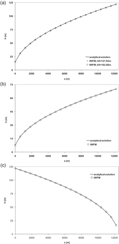
A single layer aquifer of 12 192 m in the x-direction, 12 192 m in the y-direction and 152.4 m in the z-direction is assumed. The computational domain of the model is discretized by m. The hydraulic conductivity is assumed to be 30.5 m/d and the specific yield and specific storage values are set to zero. No-flow boundary conditions are assumed at y = 0 and y = 12 192 m. The initial groundwater head is assumed to be h₀ = 121.9 m. Assuming that water flow is only in the horizontal direction and the model domain is isotropic and homogeneous, steady-state 1D flow in an unconfined aquifer is investigated using three different boundary condition alternatives (analytical solutions are presented in the Appendix):

1. two specified head boundary conditions (h_x = 0 = 15.2 m and h_{x = 12 192} = 121.9 m are assumed, where h_x = 0 is the head at x = 0 and h_{x = 12 192} is the head at x = 12 192 m);

2. specified head and specified flux boundary conditions (h_x = 0 = 7.6 m, and Q_{x = 12 192} = 3700 m³/d are assumed where Q_{x = 12 192} is the flow at x = 12 192 m); and

3. specified head and general head boundary conditions (h_x = 0 = 121.9 m and general head boundary h_GHB = 15.2 m is located 30.5 m away from the boundary at x = 12 192 m).

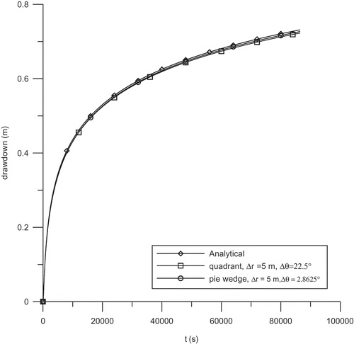
Test problem 2: Drawdown in a confined aquifer

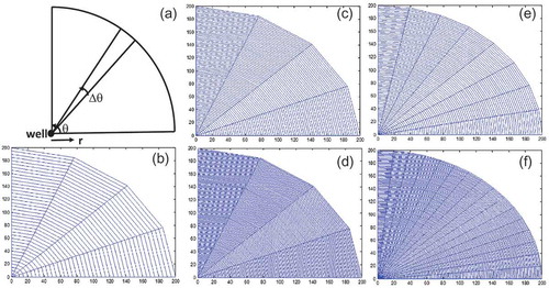
The Theis solution (Theis 1935, Bedient and Huber 1992), which is one of the most widely used analytical techniques in hydrogeology, predicts the drawdown in a confined aquifer at any distance from a well at any time since the start of pumping for a given set of aquifer properties. In this problem, the drawdown is investigated at an observation point located 55 m away from the well. Solutions for the quadrant and pie wedge domains are also investigated. In addition, different grid resolutions are formulated for each domain to investigate the grid refinement effects. Because of the symmetry, one can use different radial domains to simulate this problem. The layout of the computational domain is depicted in Figure 1(a). For the quadrant domain, the centre angle, θ, is 90° and the radius, r, is set to 20 000 m. For the pie wedge domain, θ = 11.45° and r = 20 000 m. Computational grid elements of the quadrant domain for various discretizations of dr and dθ are presented in Figure 1(b)–(f).

Figure 1. (a) Plan view of the computational domains for test problems 2 and 3. Computational grids of quadrant domain enlarged at 0 ≤ r ≤ 200 m for (b) dr = 5 m and dθ = 22.5°, (c) dr = 2.5 m and dθ = 22.5°, (d) dr = 1.25 m and dθ = 22.5°, (e) dr = 2.5 m and dθ = 11.25°, and (f) dr = 1.25 m and dθ = 5.625°.

The aquifer is assumed to be 100 m thick. Groundwater head of 150 m is assigned at 20 000 m away from the well and the initial groundwater head of 150 m is assumed at all nodes. The pumping rate is set to 0.004 m³/s (0.001 m³/s for the quadrant domain and 1.27337 × 10^–4 m³/s for the pie wedge domain). Finally, the horizontal hydraulic conductivity and the specific storage of the aquifer are set to 2.3 × 10^–5 m/s and 7.5 × 10⁻⁶ m⁻¹, respectively.

Test problem 3: Groundwater pumping in a leaky aquifer

The transient response of drawdown in a leaky aquifer due to a well with a constant discharge rate is investigated. Leaky aquifers represent a complex problem in well hydrology. When a well located in a leaky aquifer is pumped, the piezometric head in the aquifer is lowered, causing the groundwater in the overlaying aquifer to migrate vertically through the aquitard that separates the two aquifer layers. A schematic description of the groundwater pumping in a leaky aquifer is presented in Figure 2.

Figure 2. Schematic description of groundwater pumping in a leaky aquifer for test problem 3.

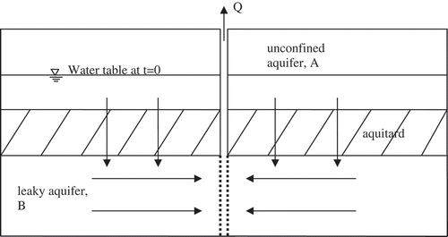
In the test problem, a quadrant domain (θ = 90°) with radius r = 20 000 m is used, in which the observation point is set 100 m away from the well (Fig. 2). The model domain is discretized by the radial increment ∆r = 5 m and the angular increment ∆θ = 22.5°. The thickness of aquifer A, the thickness of the aquitard and the thickness of aquifer B are taken as 100 m, 50 m and 50 m, respectively.

A groundwater head of 150 m is assigned at 20 000 m away from the well for both aquifer layers. The initial groundwater head is assumed to be 150 m. The pumping rate is set to 0.004 m³/s (0.001 m³/s for the quadrant domain). Finally, the horizontal and vertical hydraulic conductivity of the aquifer, the vertical hydraulic conductivity of the aquitard and the specific storage are set to 2.3 × 10^–5 m/s, 2.3 × 10^–6 m/s, 2.3 × 10^–7 m/s and 1.5 × 10^–5 m⁻¹, respectively.

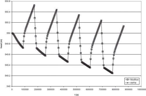
Test problem 4: Investigation of groundwater levels in a confined aquifer affected by the water storage in the inter-bed layer

The IWFM calculates the groundwater head changes due to subsidence in relation to the vertical compaction of inter-beds, which have poor permeability within a relatively permeable aquifer (CADWR 2015a). In this problem, we investigate the groundwater levels in a confined aquifer affected by the water storage in the inter-bed layer. A fully penetrating well is located in the centre of the simulation domain through which water is withdrawn and recharged in a cyclic manner. The only sources and sinks of water are the discharge or recharge through the single well and storage in the inter-bed layer and the aquifer. A schematic description of the test problem is depicted in Figure 3. A single layer aquifer is utilized as the model domain with width, length and thickness of 500 m. The inter-bed thickness is 20 m. The model domain is discretized by Δx = Δy = 5 m. The observation point is at 100 m away from the well.

Figure 3. Schematic of the aquifer with land subsidence due to groundwater pumping for Test problem 4.

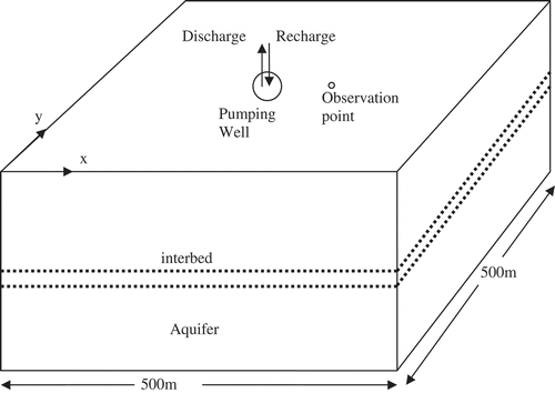
No-flow boundary conditions are assumed on all sides and bottom of the aquifer. Initial groundwater head is assumed as 550 m. The pumping rate is 0.04 m³/s on the first day and 20% of the extracted water (0.008 m³/s) is recharged through the well on the second day. This cycle is repeated five times during the 10-day simulation period.

The horizontal hydraulic conductivity, specific storage, specific yield and pre-consolidation head of the aquifer are set as 2.3 × 10^–5 m/s, 7.5 × 10^–6 m⁻¹, 0.075 and 550 m, respectively. Finally, the elastic and inelastic skeletal specific storages are taken as 5 × 10^–5 and 5 × 10^–3m⁻¹, respectively.

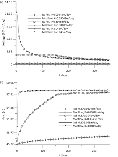
Test problem 5: Stream–aquifer interaction in a gaining unconfined aquifer

In this test problem, stream–aquifer interaction in a gaining unconfined aquifer is investigated by comparing the IWFM results with those obtained by MODFLOW. The stream–aquifer interaction in IWFM is simulated as a Cauchy boundary condition, similarly to MODFLOW (Harbaugh and McDonald 1996a). A schematic description of the model domain is shown in Figure 4(a). The width, length and thickness of the single layer aquifer utilized in this test problem are 6096, 6096 and 76.2 m. The model domain is discretized into 3481 computational elements. A stream reach that runs parallel to the y-axis is located at x = 2895.6 m. The IWFM and MODFLOW results are compared at the observation point, located at x = y = 2895.6 m.

Figure 4. Plan view of the model domains used in (a) test problem 5 (without pumping wells) and (b) test problem 6 (with four pumping wells).

No-flow boundary conditions are assumed at y = 6096 m and y = 0, while groundwater heads at x = 0 and x = 6096 m are fixed at 45.72 m. Initial groundwater head is taken as 45.72 m at all nodes. The horizontal hydraulic conductivity, specific yield and stream-bed hydraulic conductivity are taken as 30.50 m/d, 0.25 and 0.3048 m/d, respectively. The width of the stream channel and the initial streambed elevation are assumed to be 30.5 m and 57.91 m, respectively. A constant inflow to the stream is assumed to be 14.16 m³/s. Finally, Manning’s roughness and the slope of the stream channel are 0.03 and 0.0001, respectively.

Test problem 6: Reaction of streamflow to the withdrawal and the recharge of water through wells in a cyclic manner

The dimensions, physical parameters and boundary conditions of the aquifer are the same as for test problem 5. A schematic description of the model domain is depicted in Figure 4(b). Four fully penetrating wells are located at (x, y) coordinates of (3234.2 m, 2929.5 m), (3234.2 m, 2861.7 m), (2556.9 m, 2929.5 m) and (2556.9 m, 2861.7 m) in the model domain. Water is withdrawn and recharged in a cyclic manner through the wells. Withdrawal and recharge flow rates at each of the four wells through simulation time are given in Table 2. The purpose of this problem is to check if IWFM correctly captures the reaction of streamflow to withdrawal and recharge of water through the wells near a stream. A constant inflow of 14.16 m³/s is applied at the upstream boundary (located at the northern boundary of the model domain) of the stream. The initial groundwater head for the entire domain was set to 59.1 m.

Table 2. Withdrawal and recharge (m³/s) from each of the four wells through simulation time for test problem 6.

	Time (d)
	1–90	91–180	181–270	271–360	361–450	451–540	541–630	631–720
Withdrawal (m^3/s)	0	0.14158	0	0.14158	0	0.14158	0	0.14158
Recharge (m^3/s)	0	0	0.14158	0	0.14158	0	0.14158	0

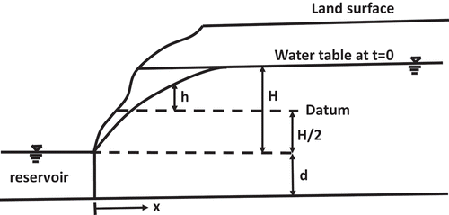
Test problem 7: Prediction of water table position through time in an unconfined aquifer from which groundwater is flowing into a surface reservoir

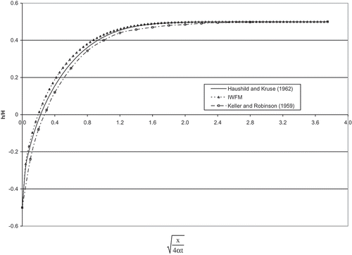
We investigated unsteady water flow with a moving free surface across a large unconfined aquifer. A schematic description of the groundwater table near a surface reservoir is demonstrated in Figure 5. The groundwater head at x = 0 is controlled by the reservoir which is located at x < 0. At time t = 0, the head is at H/2 and the head difference between the reservoir water surface and the groundwater table is H. The width, length and thickness of the single layer aquifer that are used in this test problem are 54 864 m, 60 960 m and 152.4 m, respectively. The model domain is discretized by Δx = Δy = 606.9. The reservoir level is assumed to be at the bottom of the aquifer, i.e. d = 0, and the head H is taken as 3.048 m. The head at x = 54 864 m is assumed to be 1.524 m (H/2 from datum) and no-flow boundary conditions are assumed at y = 60 960 m and y = 0. The horizontal hydraulic conductivity and specific yield are taken as 895.4 m/d and 0.255, respectively. The simulation is performed for 5000 days with time increments of 1 day. The aim in this problem is to predict water table position in the aquifer through time. An approximate method given by Haushild and Kruse (1962) and experimental data given by Keller and Robinson (1959) are compared with the results of IWFM.

Figure 5. Schematic description of groundwater table near a surface reservoir for test problem 7 (Keller and Robinson 1959, Haushild and Kruse 1962).

Results and discussion

Test problem 1

For test problems 1a, 1b and 1c, steady-state groundwater heads along the x-direction computed by IWFM and by the analytical solutions presented in the Appendix are depicted in Figure 6(a)–(c), respectively. Steady-state IWFM solutions are identical to analytical ones. Steady-state solutions of groundwater heads along the x-direction for initial groundwater heads of h₀ = 121.9 m and h₀ = 182.88 m, are plotted in Figure 6(a). As expected, the initial groundwater head did not affect the steady-state solution.

Figure 6. Groundwater head h (m) vs spatial location x (m) for test problems 1a, 1b and 1c.

Test problem 2

Figure 7 illustrates the drawdown vs time at the observation point 55 m away from the well that the test is plotted in, indicating that IWFM results fit well with the analytical solution (Theis 1935, Bedient and Huber 1992) for both quadrant and pie wedge domains. In Table 3, for different grid resolutions in the radial direction, the normalized root mean square error (NRMSE) values for the quadrant domain with angular increment of ∆θ = 22.5° and for the pie wedge domain with angular increment of ∆θ = 2.8625° are given. NRMSE is defined as:

(4)

Table 3. NRMSE values for quadrant and pie wedge domains.

∆r (m)	NRMSE values for quadrant domain	NRMSE values for pie wedge domain
5	1.09 × 10^–2	7.04 × 10^–3
2.5	6.26 × 10^–3	2.13 × 10^–3
1.25	5.06 × 10^–3	8.30 × 10^–4
0.625	4.51 × 10^–3	–
0.3125	4.34 × 10^–3	–

Figure 7. Drawdown versus time at the observation point that is located 55 m away from the well for quadrant and pie wedge domains for test problem 2.

where are the analytical or experimental values and are the simulated ones.

According to Table 3, the NRMSE values are smaller for the pie wedge domain than for the quadrant domain, probably due to smaller cell sizes in the pie wedge domain. Moreover, NRMSE values for the quadrant domain do not converge to zero as the radial grid resolution (∆r) becomes finer for a fixed angular grid resolution. The same behaviour was also observed when grid resolution in the angular direction was refined systematically for a fixed grid resolution in the radial direction. The lack of fast convergence of NRMSE to zero when either angular grid or radial grid resolution is refined while the other is kept constant can be explained by the concept of grid cell aspect ratio. The latter is defined as the ratio of the length of the longest side of the cell to the length of its shortest side. The disadvantages of finite elements with high aspect ratios have been documented in Mittal (2000). As shown in Table 3, as the radial grid resolution is refined for the quadrant domain while angular resolution is kept constant, the aspect ratio of grid cells increases, thus adversely affecting the convergence of the IWFM results to the analytical solution.

To further clarify this point, we provide in Table 4 the NRMSE for the quadrant domain when grid resolution in both radial and angular directions is modified by keeping the aspect ratio of the grid cells constant. It is shown that almost quadratic convergence is achieved when grid resolution is halved in both directions while keeping the cell aspect ratio constant.

Table 4. NRMSE values for quadrant domain for constant aspect ratio of mesh elements.

∆r (m)	∆θ (°)	NRMSE
5	22.5	0.0109
2.5	11.25	0.0028
1.25	5.625	0.0008

Test problem 3

For test problem 3, the drawdown values in a leaky aquifer vs time at 100 m away from the well for computational time steps of 100, 1000 and 10 000 s are tabulated in Table 5. The IWFM results are compared against the approximate solution proposed by Hantush and Jacob (1955). NRMSE values are calculated as 0.009, 0.011 and 0.037 for time steps of 100, 1000 and 10 000 s, respectively. As expected, employing finer time steps results in better predictions of drawdown.

Table 5. Drawdown (m) in a leaky aquifer vs time at 100 m away from the pump, for different time steps for test problem 3.

Time (s)	Drawdown (m)
	Benchmark (Hantush and Jacob 1955)	IWFM ∆t = 100	∆t = 1000	∆t = 10 000
10 000	3.75 × 10^–1	3.68 × 10^–1	3.59 × 10^–1	2.92 × 10^–1
20 000	5.31 × 10^–1	5.24 × 10^–1	5.19 × 10^–1	4.67 × 10^–1
30 000	6.22 × 10^–1	6.14 × 10^–1	6.11 × 10^–1	5.73 × 10^–1
40 000	6.83 × 10^–1	6.76 × 10^–1	6.73 × 10^–1	6.44 × 10^–1
50 000	7.28 × 10^–1	7.21 × 10^–1	7.19 × 10^–1	6.95 × 10^–1
60 000	7.63 × 10^–1	7.56 × 10^–1	7.54 × 10^–1	7.35 × 10^–1
70 000	7.91 × 10^–1	7.83 × 10^–1	7.82 × 10^–1	7.66 × 10^–1
80 000	8.14 × 10^–1	8.06 × 10^–1	8.05 × 10^–1	7.91 × 10^–1
90 000	8.33 × 10^–1	8.25 × 10^–1	8.24 × 10^–1	8.12 × 10^–1
100 000	8.49 × 10^–1	8.41 × 10^–1	8.40 × 10^–1	8.29 × 10^–1
200 000	9.29 × 10^–1	9.19 × 10^–1	9.19 × 10^–1	9.15 × 10^–1
300 000	9.53 × 10^–1	9.44 × 10^–1	9.44 × 10^–1	9.42 × 10^–1
400 000	9.63 × 10^–1	9.55 × 10^–1	9.55 × 10^–1	9.54 × 10^–1
500 000	9.67 × 10^–1	9.60 × 10^–1	9.60 × 10^–1	9.59 × 10^–1
600 000	9.69 × 10^–1	9.63 × 10^–1	9.63 × 10^–1	9.63 × 10^–1
700 000	9.70 × 10^–1	9.65 × 10^–1	9.65 × 10^–1	9.65 × 10^–1
800 000	9.70 × 10^–1	9.67 × 10^–1	9.67 × 10^–1	9.67 × 10^–1
900 000	9.70 × 10^–1	9.69 × 10^–1	9.69 × 10^–1	9.69 × 10^–1
1 000 000	9.70 × 10^–1	9.70 × 10^–1	9.70 × 10^–1	9.70 × 10^–1
2 000 000	9.70 × 10^–1	9.83 × 10^–1	9.83 × 10^–1	9.83 × 10^–1
NRMSE	–	9.00 × 10^–3	1.10 × 10^–2	3.70 × 10^–2

Test problem 4

The IWFM results are compared with the results obtained by MODFLOW-96 (Harbaugh and McDonald 1996a, b). The model grids are generated such that vertices of the IWFM finite element grid cells are located at the centres of the MODFLOW grid cells. The response of the groundwater head observed at 100 m away from the well to cyclic discharge and recharge as simulated by MODFLOW and IWFM are shown in Figure 8. The groundwater heads estimated by IWFM match well with those estimated by MODFLOW. Figure 8 also depicts the interaction of inter-bed storage with the aquifer system. It can be observed that the groundwater head drop during pumping periods is less than the head increase during recharge periods.

Figure 8. Head (m) versus time (s) at the observation point located 100 m away from the well for test problem 4.

Test problem 5

The IWFM results are compared with the results obtained by MODFLOW-96 (Harbaugh and McDonald 1996a, b). Similar to test problem 4, the vertices of the IWFM grid cells are located at the centres of the MODFLOW grid cells to facilitate an easier comparison of the two model results. The total stream leakage and groundwater heads at the observation point, which is located in the middle of the stream reach (Fig. 4(a)), considering three different stream bed hydraulic conductivity values (K = 0.03048, 0.3048, 3.048 m/d) are illustrated in Figure 9(a) and (b), respectively. IWFM predictions of stream leakage and groundwater heads match the MODFLOW counterparts quite well for all of the three hydraulic conductivity values. The NRMSE values for groundwater heads at the observation point and leakage from the stream are tabulated in Table 6. The maximum NRMSE values are 4.20 × 10^–4 for the groundwater head at the observation point and 6.89 × 10^–3 for the leakage. At the beginning of simulation, the stream leakage is highest for K = 3.048 m/d and lowest for K = 0.03048 m/d (Fig. 9(a)). Stream leakage decreases exponentially when K = 3.048 m/d because, as the groundwater head increases due to stream leakage, the elevation difference between groundwater head and stream surface decreases exponentially (Fig. 9(b)). For K = 0.3048 m/d, the groundwater and stream are hydraulically disconnected (i.e. groundwater head is below the stream bed elevation) until around t = 150 days, at which point groundwater heads have reached to the stream bottom (Fig. 9(b)). After this point, the stream leakage decreases as the groundwater heads increase further until equilibrium is reached. At the end of simulation, the stream leakage and groundwater level for K = 0.3048 and K = 3.048 m/d reach a constant value at which groundwater and stream are in equilibrium (Fig. 9(a)). In contrast, the stream leakage is the smallest for K = 0.03048 m/d and the groundwater heads is below the stream bed during the entire simulation period, leading to a constant stream leakage value. However, the constantly increasing groundwater head when K = 0.03048 m/d (Fig. 9(b)) suggests that if the simulation period is extended, it is likely that both stream leakage and groundwater levels would reach an equilibrium even for this case.

Table 6. NRMSE values for groundwater heads at observation point and total stream leakage for test problem 5.

	K = 0.030 48 m/d	K = 0.3048 m/d	K = 3.048 m/d
Head	4.20 × 10^–4	9.30 × 10^–5	1.01 × 10^–4
Leakage	2.40 × 10^–5	6.89 × 10^–3	5.97 × 10^–3

Figure 9. Time variation of (a) stream leakage and (b) groundwater head at the observation point (in the middle of the stream reach) estimated by IWFM and MODFLOW for test problem 5.

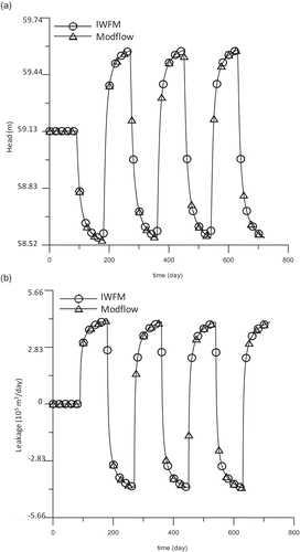
Test problem 6

The groundwater heads at the observation point (in the middle of the stream reach) and the stream leakage through time due to the withdrawal and the recharge of water through four wells in a cyclic manner are plotted in Figure 10(a) and (b), respectively. A negative leakage represents a gaining stream, whereas a positive leakage represents a losing stream. IWFM predictions of heads and leakage values are identical with the MODFLOW counterparts. For the 90-day period, both withdrawal and recharge rates at the wells are zero so initial head at the observation point is constant and stream leakage is zero. When pumping is turned on, the groundwater head at the observation point decreases and the stream leakage increases, as shown in Figure 10(a) and (b), respectively, thus turning the stream into a losing stream. However, when the aquifer is recharged, the groundwater head at the observation point increases and the stream becomes a gaining stream, since the leakage becomes negative.

Figure 10. Time variation of (a) groundwater head and (b) stream leakage at the observation point for test problem 6.

Test problem 7

Measurements of a drawdown curve in a laboratory flume filled with sand, which was obtained by Keller and Robinson (1959), and the approximate solution given by Haushild and Kruse (1962), referred to as solution IV, are compared with IWFM results. Solution IV is given by:

(5)

where:

(6)

(7)

Here ϕ is the error function given by:

(8)

where α = KD/V and t, K and V are the time, the horizontal hydraulic conductivity of the aquifer and the specific yield, respectively.

In Figure 11 the dimensionless head h/H is plotted versus , for t = 5000 d. The reservoir level is assumed to be at the bottom of the aquifer, i.e. d = 0, so that approximation of IWFM can also be compared with the experimental data by Haushild and Kruse (1962). Solution IV by Haushild and Kruse (1962) over-predicts the experimental data by Keller and Robinson (1959). Although the results obtained by IWFM are slightly larger than those of Haushild and Kruse, they are in overall acceptable agreement with the experimental ones.

Figure 11. Computed dimensionless water table profile and experimental data for test problem 7.

Summary and conclusions

Very little formal verification and/or benchmarking of hydrological models that are capable of simulating integrated surface and subsurface flow has been performed. This study was an attempt to perform verification of the groundwater module of the IWFM through several benchmark test problems. This study also presented some of the potential usage and capabilities of the IWFM. The capability of the IWFM in simulating various hydrological processes under different boundary conditions was examined utilizing one- and two-dimensional hypothetical test problems. The test problems cover a wide range of hydrological and boundary conditions.

In test problem 1, the steady-state groundwater heads computed by IWFM and by the analytical solutions were compared in an unconfined aquifer under various boundary conditions. In the next problem, IWFM simulations of temporal change of drawdown in a confined aquifer were compared with the Theis solution. Results for quadrant and pie wedge domains were also investigated. Moreover, different grid resolutions were formulated for each domain to explore the grid refinement effects, and grid-cell aspect ratio. It was shown that almost quadratic convergence was achieved when grid resolution was halved in both radial and angular directions while keeping the cell aspect ratio constant. On other hand, it was shown that grid refinement in one direction, which results in increasing grid aspect ratio, was not so successful.

In test problem 3, IWFM simulations of the transient response of drawdown in a leaky aquifer due to a well with a constant discharge were compared against the approximate solution proposed by Hantush and Jacob (1955). It was demonstrated that employing finer time steps results in better predictions of drawdown. In test problem 4, we investigated MODFLOW and IWFM simulations of the groundwater levels in a confined aquifer affected by the water storage in the inter-bed layer and a fully penetrating well through which water is withdrawn and recharged in a cyclic manner. In test problem 5, the stream–aquifer interaction in a gaining unconfined aquifer was investigated for various streambed hydraulic conductivities by comparing the IWFM and MODFLOW simulations of total stream leakage and groundwater heads at an observation point. Then, reaction of streamflow, as a gaining stream or a losing stream, to the withdrawal and the recharge of water through four fully penetrating wells in a cyclic manner was examined by comparing the IWFM and MODFLOW simulations.

Finally, in the last test problem, we investigated unsteady water flow with a moving free surface across a large unconfined aquifer from which groundwater is flowing into a surface reservoir. Here, an approximate solution (Haushild and Kruse 1962) and experimental data given by Keller and Robinson (1959) were compared with the results of IWFM.

In all of the test problems, IWFM predictions performed quite well compared to the analytical solutions, field/laboratory observations, or results from MODFLOW runs when neither analytical solutions nor observed data were available. In conclusion, the groundwater module of IWFM could be a useful tool for engineers, modellers and researchers in water resources modelling and the management community. At the moment, IWFM is a strong candidate as a modelling tool in aiding California’s water districts to comply with the recently passed Sustainable Groundwater Management Act (SGMA). In the future, the performance of the other components of the IWFM will also be investigated.

Acknowledgements

The authors would like to thank two anonymous reviewers and the Associate Editor, Dr Andreas Efstratiadis, for their valuable comments and suggestions, which have led to significant improvement on the quality of this paper.

Disclosure statement

No potential conflict of interest was reported by the authors.

APPENDIX: Analytical solutions for test problems 1a, 1b and 1c

The governing equation for unconfined and homogeneous aquifers at steady state (Wang and Anderson 1982) is:

(A1)

Since there is no head gradient in the y-direction for test problem 1, Equation (A1) reduces to:

(A2)

Integrating Equation (A2) twice and taking the square root of the resulting expression, we obtain:

(A3)

Since the head is specified at x = 0 at h_{x = 0}, for all of tests we get:

(A4)

For each test, using the boundary conditions at x = L_x, c₁ is estimated as follows:

Test 1a

Since the constant head at x = L_x is h_{x = Lx}, after substitution, Equation (A3) can be solved for c₁:

(A5)

Substituting Equations (A4) and (A5) into Equation (A3), we obtain:

(A6)

Test 1b

Using the Darcy law under the Dupuit assumption, the specified flux at x = L_x can be written as (Dupuit 1863):

(A7)

Rearranging Equation (A7) and using Equation (A3) to express the derivative of h², c₁ can be expressed as:

(A8)

Substitution of Equations (A4) and (A8) into Equation (A3) gives the solution for h:

(A9)

Test 1c

The general head boundary (GHB) condition at x = L _x can be expressed as (CADWR 2015a):

(A10)

where K, A and d are the hydraulic conductivity of the aquifer at the boundary, cross-sectional area at the boundary that flow passes through, and the distance between the boundary and the location of the known head, respectively. Using the Darcy law under the Dupuit assumption at x = L_x:

(A11)

where l is the length of the boundary where the general head boundary condition is specified. By substituting at from Equation (A3), and into Equation (A11), we obtain the following implicit equation for c₁:

(A12)

Equation (A12) is a quadratic equation and can be solved iteratively. When solved for c₁, Equation (A12) provides two solutions; however, only one of them is acceptable, since the other solution produces head values that are physically unrealistic. Then, h can be solved using c₁ and c₂ in Equation (A3).

References

- Allen, R.G., et al., 1998. Crop evapotranspiration - Guidelines for computing crop water requirements: Food and Agriculture Organization of the United Nations, Irrigation and Drainage Paper 56, 300 p.
- Andersen, P.F., 1993. A manual for Instructional Problems for the USGS MODFLOW Model. Publication No. EPA/600/R-93/010. Available from: http://nepis.epa.gov/Exe/ZyPURL.cgi?Dockey=2000BHNI.txt [ Accessed June 2015].
- BCDWRC (Butte County Department of Water and Resource Conservation). 2004. Butte Basin groundwater model update: Phase I Report, 57 p. Available from: http://www.buttecounty.net/Portals/26/Modeling/DWRC-Strategic-Plan-2011-2015.pdf [ Accessed September 2014].
- BCDWRC (Butte County Department of Water and Resource Conservation). 2008a. Butte Basin groundwater model update: Phase II Report, 155 p. Available from: http://www.buttecounty.net/Portals/26/Modeling/CDM%20Butte%20Basin%20Model%20TM2%20FINAL.pdf [ Accessed September 2014].
- BCDWRC (Butte County Dept. Water and Resource Conservation). 2008b. Butte Basin groundwater model update: Base case and water management scenario simulations, 25 p. Available from: http://www.buttecounty.net/Portals/26/Modeling/TM3BaseCaseScenario20080424.pdf [ Accessed September 2014].
- Bedient, P.B. and Huber, W.C., 1992. Hydrology and flood plain analysis. 2nd edn. Addison-Wesley publishing company, p. 692. ISBN: 9780201517118.
- Bellin, A., et al., 2016. A continuous coupled hydrological and water resources management model. Environmental Modelling & Software, 75, 176–192. doi:10.1016/j.envsoft.2015.10.013.
- Brush, C.F. and Dogrul, E.C., 2013. User manual for the California Central Valley groundwater-surface water simulation model (C2VSim), version 3.02-CG. Available from: http://baydeltaoffice.water.ca.gov/modeling/hydrology/C2VSim/download/C2VSim_Users_Manual_Final.pdf [ Accessed September 2014].
- Brush, C.F., Dogrul, E.C., and Kadir, T.N., 2013. DWR technical memorandum: development and calibration of the California Central Valley groundwater-surface water simulation model (C2VSim), version 3.02-CG. Available from: http://baydeltaoffice.water.ca.gov/modeling/hydrology/C2VSim/download/C2VSim_Model_Report_Final.pdf [ Accessed September 2014].
- CADWR (California Department of Water Resources). 2015a. Integrated Water Flow Model (IWFM-2015): Theoretical Documentation. Central Valley Modeling Unit, Modeling Support Branch, Bay-Delta Office, Sacramento. Available from: http://baydeltaoffice.water.ca.gov/modeling/hydrology/IWFM/IWFM-2015/v2015_0_260/downloadables/IWFM-2015.0.260_TheoreticalDocumentation.pdf [ Accessed May 2015].
- CADWR (California Department of Water Resources). 2015b. IWFM Demand Calculator (IDC-2015): Theoretical Documentation and User’s Manual, Central Valley Modeling Unit, Modeling Support Branch, Bay-Delta Office, Sacramento. Accessed from: http://baydeltaoffice.water.ca.gov/modeling/hydrology/IDC/IDC-2015/v2015_0_36/downloadables/IDC-2015.0.36_Documentation.pdf [ Accessed May 2015].
- Campbell, G.S., 1974. A simple method for determining unsaturated conductivity from moisture retention data. Soil Science, 117 (6), 311–314. doi:10.1097/00010694-197406000-00001
- Dale, L.L., et al., 2013. Simulating the impact of drought on California’s Central Valley hydrology, groundwater and cropping. British Journal of Environment and Climate Change, 3 (3), 271–291. doi:10.9734/BJECC/2013/2680
- Danish Hydraulic Institute (DHI), 1999. Mike She pre- and post-processing user manual. Hørsholm, Denmark: DHI Software.
- Dogrul, E.C., et al., 2016. Linking groundwater simulation and reservoir system analysis models: the case for California’s Central Valley. Environmental Modelling & Software, 77, 168–182. doi:10.1016/j.envsoft.2015.12.006
- Dogrul, E.C., Kadir, T.N., and Chung, F.I., 2011. Root zone moisture routing and water demand calculations in the context of integrated hydrology. Journal of Irrigation and Drainage Engineering, 137 (6), 359–366. doi:10.1061/(ASCE)IR.1943-4774.0000306
- Draper, A.J., et al., 2004. CalSim: Generalized model for reservoir system analysis. Journal of Water Resources Planning and Management, 130 (6), 480–489. doi:10.1061/(ASCE)0733-9496(2004)130:6(480)
- Dupuit, J., 1863. Etudes Théoriques et Pratiques sur le Mouvement des Eau x dans les Canau x Découverts et a Travers les Terrains Perméables. 2nd edn. Paris: Dunod.
- Efstratiadis, A., et al., 2008. Hydrogeios: a semi-distributed GIS-based hydrological model for modified river basins. Hydrology and Earth System Sciences, 12, 989–1006. doi:10.5194/hess-12-989-2008
- Ercan, A., 2006. Verification problems for IWFM. Department of Water Resources, Bay-Delta Office, Modeling Support Branch, 42 p. Available from: http://baydeltaoffice.water.ca.gov/modeling/hydrology/IWFM/Publications/downloadables/Reports/IWFM_Verification.pdf [ Accessed September 2014].
- Hantush, M.S. and Jacob, C.E., 1955. Non-steady radial flow in an infinite leaky aquifer. Transactions, American Geophysical Union, 36, 95–100. doi:10.1029/TR036i001p00095
- Harbaugh, A.W. and McDonald, M.G., 1996a. User’s documentation for MODFLOW-96- An update to the U.S. Geological Survey modular finite-difference ground-water flow model, USGS Open-File Report 96-485. Available from: http://water.usgs.gov/software/code/ground_water/modflow/doc/ofr96485.pdf [Accessed July 2016].
- Harbaugh, A.W. and McDonald, M.G., 1996b. Programmer’s documentation for MODFLOW-96, an update to the U.S. Geological Survey modular finite-difference ground-water flow model, USGS Open-File Report 96-486. Available from: http://water.usgs.gov/software/code/ground_water/modflow/doc/ofr96486.pdf [Accessed July 2016].
- Harter, T. and Morel-Seytou X, H., 2013. Peer review of the IWFM, MODFLOW and HGS model codes: potential for water management applications in California’s central valley and other irrigated groundwater basins. Final Report, California Water and Environmental Modeling Forum, August 2013, Sacramento. Available from: http://www.cwemf.org/Pubs/GWModelsPeerReviewFinal.pdf [ Accessed September 2014].
- Hatchett, S., Mann, R., and Zhang, B., 1997. Analysis of agricultural economics for the central valley project improvement act programmatic environmental impact statement. Presented at Western Agricultural Economics Association 1997, annual meeting, 13–16 July Reno/Sparks, NV.
- Haushild, W. and Kruse, G., 1962. Unsteady Flow of Ground Water into a Surface Reservoir. Transactions, ASCE, 127, Part I, 408–415.
- Howitt, R.E., et al., 2014. Economic analysis of the 2014 drought for California agriculture. Center for Watershed Sciences, University of California, Davis, California. 20p. Available from: https://watershed.ucdavis.edu/files/biblio/DroughtReport_23July2014_0.pdf [ Accessed September 2014].
- Idaho Water Resources Board (IWRB), 2010. Treasure Valley future water demand, 74 p. Available from: http://www.idwr.idaho.gov/WaterBoard/WaterPlanning/CAMP/TV_CAMP/PDF/2010/09-29-2010_Water_Demand.pdf [ Accessed September 2014].
- Kavvas, M.L., et al., 2004. Watershed environmental hydrology (WEHY) model, based on upscaled conservation equations: hydrologic module. Journal of Hydrological Engineering, 9 (6), 450–464. doi:10.1061/(ASCE)1084-0699(2004)9:6(450)
- Kavvas, M.L., et al., 2006. Watershed environmental hydrology model: environmental module and its application to a California watershed. Journal of Hydrological Engineering, 11 (3), 261–272. doi:10.1061/(ASCE)1084-0699(2006)11:3(261)
- Keller, J. and Robinson, A.R., 1959. Model study of interceptor drains. Proceedings. ASCE, September, 25–40.
- Leavesley, G.H., et al., 1983. Precipitation-runoff modeling system: user’s manual. Denver, CO: US Geological Survey. 207 p. Water Resources Investigations Report 83-4238.
- Markstrom, S.L., et al., 2008. GSFLOW–coupled groundwater and surface water FLOW model based on the integration of the precipitation-runoff modeling system (PRMS) and the modular groundwater flow model (MODFLOW-2005). Reston, VA: US Geological Survey. 240 p. Techniques and Methods 6-D1.
- Maxwell, R.M., et al., 2014. Surface-subsurface model intercomparison: a first set of benchmark results to diagnose integrated hydrology and feedbacks. Water Resources Research, 50, 1531–1549. doi:10.1002/2013WR013725.
- Miller, N.L., et al., 2009. Drought resilience of the California central valley surface-ground-water-conveyance system. JAWRA Journal of the American Water Resources Association, 45 (4), 857–866. doi:10.1111/jawr.2009.45.issue-4
- Mittal, S., 2000. On the performance of high aspect ratio elements for incompressible flows. Computer Methods in Applied Mechanics & Engineering, 188 (1–3). 21 July 2000, pp. 269–287. doi:10.1016/S0045-7825(99)00152-8
- Nalbantis, I., et al., 2011. Holistic versus monomeric strategies for hydrological modelling of human-modified hydrosystems. Hydrology and Earth System Sciences, 15 (3), 743–758. doi:10.5194/hess-15-743-2011
- Refsgaard, J.C. and Henriksen, H.J., 2004. Modelling guidelines––terminology and guiding principles. Advances in Water Resources, 27 (1), 71–82. doi:10.1016/j.advwatres.2003.08.006
- Scherberg, J., et al., 2014. Design of managed aquifer recharge for agricultural and ecological water supply assessed through numerical modeling. Water Resources Management, 28, 4971–4984. doi:10.1007/s11269-014-0780-2
- Schmid, W., et al., 2006. User guide for the farm process (FMP1) for the US Geological Survey’s modular three-dimensional finite-difference groundwater flow model, MODFLOW-2000. (Book 6). Reston, VA: US Geological Survey. 127 p. Techniques and Methods 6-A17. Available from: http://pubs.usgs.gov/tm/2006/tm6A17/ [ Accessed September 2014].
- Schroeder, P.R., et al., 1994. The Hydrologic Evaluation of Landfill Performance (HELP) Model: Engineering Documentation for Version 3, EPA/600/R-94/168b. U.S. Environmental Protection Agency Office of Research and Development, Washington, DC.
- Sophocleous, M.A., et al., 1999. Integrated numerical modeling for basin-wide water management: the case of the Rattlesnake Creek basin in south-central Kansas. . Journal of Hydrology, 214 (1–4), 179–196. doi:10.1016/S0022-1694(98)00289-3
- Sustainable Groundwater Management Act (SGMA), 2014. Cal. Assembly B. 1379,C.S.B., and Cal. Senate B. 1319 [online]. Available from: https://www.opr.ca.gov/docs/2014_Sustainable_Groundwater_Management_Legislation_092914.pdf [Accessed 4 January 2016].
- Theis, C.V., 1935. The relation between the lowering of the Piezometric surface and the rate and duration of discharge of a well using ground-water storage. . Transactions, American Geophysical Union, 16, 519–524. doi:10.1029/TR016i002p00519
- Therrien, R., et al., 2010. HydroGeoSphere—a three-dimensional numerical model describing fully-integrated subsurface and surface flow and solute transport (Draft), October 2010. Available from: http://www.ggl.ulaval.ca/fileadmin/ggl/documents/rtherrien/hydrogeosphere.pdf [Accessed July 2016].
- Van Genuchten, M.T., 1980. A closed-form solution for predicting the conductivity of unsaturated soils. Soil Science Society of America Journal, 44, 892–898. doi:10.2136/sssaj1980.03615995004400050002x
- Wang, H.F. and Anderson, M.P., 1982. Introduction to groundwater modeling: finite difference and finite element methods. San Diego, CA: Academic Press.