Evaluation of storage–discharge relationships and recession analysis-based distributed hourly runoff simulation in large-scale, mountainous and snow-influenced catchment

ABSTRACT

Evaluation of a recession-based “top-down” model for distributed hourly runoff simulation in macroscale mountainous catchments is rare in the literature. We evaluated such a model for a 3090 km² boreal catchment and its internal sub-catchments. The main research question is how the model performs when parameters are either estimated from streamflow recession or obtained by calibration. The model reproduced observed streamflow hydrographs (Nash-Sutcliffe efficiency up to 0.83) and flow duration curves. Transferability of parameters to the sub-catchments validates the performance of the model, and indicates an opportunity for prediction in ungauged sites. However, the cases of parameter estimation and calibration excluding the effects of runoff routing underestimate peak flows. The lower end of the recession and the minimum length of recession segments included are the main sources of uncertainty for parameter estimation. Despite the small number of calibrated parameters, the model is susceptible to parameter uncertainty and identifiability problems.

EDITOR D. Koutsoyiannis; ASSOCIATE EDITOR A. Carsteanu

KEYWORDS:

• Distributed hourly runoff
• storage–discharge relationships
• streamflow recession
• discharge sensitivity function
• boreal catchments
• source-to-sink routing

1 Introduction

Continuous simulation of runoff in gauged and ungauged watersheds is important in water resources management for objectives such as flood forecasting, design and operation of water infrastructure and ecological assessments. However, several studies have indicated the uniqueness of catchment runoff responses due to natural heterogeneities in catchment characteristics, climate forcing, dominant hydrological processes and process interactions (e.g. Beven 2000, McDonnell et al. 2007), which complicates the application of simulation models.

A plethora of precipitation–runoff models based on various modelling approaches have been developed to conceptualize dominant hydrological processes in catchments (e.g. Singh and Woolhiser 2002). Various lumped conceptual precipitation–runoff modelling strategies, for instance linear or nonlinear reservoir-based models (e.g. Bergström 1976) or fill-and-spill storage-based models with parameterization of sub-basin heterogeneity by a probability distribution (e.g. Moore 1985), are widely employed, especially for operational forecasting purposes, due to their lower requirements for data and simplicity of updating model states. Despite their advantages, it is argued that these models rely heavily on parameter tuning using calibration algorithms, which may increase problems related to parameter uncertainty and identifiability.

Another modelling approach commonly employed in hydrological sciences is based on modelling the dominant hydrological processes from point-scale physical equations and upscaling to larger scales following the “bottom-up” approach (Klemeš 1983, Jarvis 1993). One of the main motivations for the distributed process-based “bottom-up” models was to reduce parameter calibration efforts by parameterizing in terms of measurable physical quantities. However, in practice, effective values of parameters are set by calibration to compensate for the limitations of the approximation to the physics of flow in heterogeneous domains (see Beven 2000). This domain of models also better represent the spatial variability of inputs and processes, and are applicable in assessing the impacts of land use and climate change. For a model to be fully distributed, all aspects of the model must be distributed, including parameters, initial and boundary conditions, and sources and sinks (Singh and Woolhiser 2002). Therefore, distributed models require more data than lumped models. Cunderlik et al. (2013) noted that the full potential of distributed models could only be realized under particular logistical circumstances.

The “top-down” (Klemeš 1983, Jarvis 1993) precipitation–runoff modelling approach is also common in hydrology. According to Sivapalan et al. (2003), the defining feature of this approach is that it attempts to predict the overall catchment response based on an interpretation of the observed response at the catchment scale. The authors also noted the importance of this approach for parameter parsimony and learning from observed data. Kirchner (2009) suggested a recession-based “top-down” approach for lumped rainfall–runoff modelling based on “catchments as simple dynamical systems”, in which the combined effect of all subsurface flow processes on discharge (Q) of the catchment can be represented as resulting from a single variable of bulk catchment storage (S), and the conceptualization of the system properties can be inferred from temporal fluctuations in streamflow during recession. Kirchner inferred model structure, equations and parameters by analysing streamflow recessions to reduce reliance on traditional parameter tuning by calibration, which is challenging in overparameterized and poorly identified models. Kirchner also demonstrated lumped modelling methodology for headwater catchments in Mid-Wales (United Kingdom) for both parameter estimation from streamflow recession analysis and from direct calibration based on observed rainfall–runoff relationships. Teuling et al. (2010) demonstrated good performance of the approach for streamflow simulation during wet periods in a snow-influenced Swiss pre-alpine catchment. Rainfall–runoff modelling based on storage–discharge relationships and streamflow recession analysis has been applied for a long time (e.g. Lambert 1969, Ambroise et al. 1996, Lamb and Beven 1997, Wittenberg and Sivapalan 1999, Rees et al. 2004, Aksoy and Wittenberg 2011 and Fiorotto and Caroni 2013).

The main basis of the approach by Kirchner (2009) is the water balance equation. The author inferred a single-storage model structure based on a discharge sensitivity function, g(Q) = dQ/dS. If discharge is a function of storage, then the catchment antecedent moisture will be measured implicitly by stream discharge and the catchment response to a unit increase in storage will be directly quantified by the hydrological sensitivity function (Kirchner 2009). The main assumptions in the approach are that the discharge from the catchment (Q) depends solely on the release of water from storage in the catchment (S) rather than “bypassing” flow from direct precipitation, and the S–Q relationship is a monotonically increasing function and is invertible, i.e. Q = f(S); S = f⁻¹(Q). The unsaturated and saturated storages are assumed to be hydraulically connected. In addition, the net groundwater flow across the watershed boundary is assumed to be zero.

There are several advantages in this approach:

1. It does not specify the functional form of the storage–discharge relationship a priori, but rather determines it directly from analysis of streamflow fluctuations.

2. Parameters can be estimated from streamflow recession, e.g. during night-time low-flow periods, when the effects of evapotranspiration and precipitation are assumed negligible, which reduces the reliance on uncertain and unrepresentative climate data for parameter calibration.

3. The method allows parameter estimation from recession analysis and hence reduction of calibrated parameters, which improves parameter identifiability.

4. Inferences on catchment storage can be made from readily available streamflow observations. We are particularly limited by our inability to “see” the subsurface of a catchment, in which much of the hydrological response often remains hidden from our current measurement techniques (Wagener et al. 2007). In this regard, Ajami et al. (2011) applied the recession approach to estimate mountain block recharge (MBR) in a semi-arid region.

5. The S–Q relationship is invertible and allows effective rainfall inputs and evapotranspiration rates to be inferred from the fluctuations in discharge. Beven (2012) noted that a more interesting application of the recession-based approach is to infer effective rainfall inputs and evapotranspiration rates from the fluctuations in discharge. Krier et al. (2012) illustrated inference of basin-averaged effective precipitation rates from streamflow fluctuations for 24 small to mesoscale (<1092 km²) catchments of heterogeneous lithology.

There are also limitations on the recession-based approach due to the assumptions on which it was derived. The main limitations (Kirchner 2009) are that the method cannot be expected to give reasonable results in catchments in which the infiltration excess runoff mechanism is dominant, in catchments where runoff is controlled by interconnected subsurface reservoirs with different storage–discharge relationships, in small catchments where streams are not permanent, and in large-scale catchments where rainfall–runoff behaviour is determined more by the spatial distribution of precipitation and the runoff delay in the hillslope and channel networks than by the storage–discharge dynamics.

Kirchner (2009) concluded with the importance of assessing the applicability of the recession-based approach to diverse hydrological settings. Previous studies (e.g. Sivapalan et al. 2003, Blöschl 2006) also suggested the need for testing models in many catchments exhibiting different climatic and hydrological conditions to evaluate the applicability of the model. Relevant to the boreal catchment under study, Myrabo (1997), Beldring (2002) and Jansson et al. (2005) noted that the dominant soil formation in boreal catchments is glacial tills, in which the dominance of preferential flow has been reported (e.g. Jansson et al. 2005). However, Zehe and Sivapalan (2009) classified preferential flow and connectivity of flow paths to the outlet as runoff response thresholds. Therefore, dominance of preferential flows in glacial tills has the potential to violate one of the main assumptions of the recession-based model: the assumption of hydraulic connectivity of unsaturated and saturated storage. In addition, the storage–discharge relationship that characterizes the overall catchment behaviour might not describe any individual point on the landscape (Kirchner 2009), which is a limitation of any spatially lumped precipitation–runoff model. Several studies have also illustrated the non-uniqueness of the response of discharge to storage. For instance, Clark et al. (2009) illustrated, for a mountain watershed in Georgia (USA), that the recession relationship of (dQ/dt) and Q is approximately consistent with a linear reservoir at hillslope scale, and deviation from linearity becomes progressively larger with increasing spatial scale. Myrabo (1997), Beven (2006), Ewen and Birkinshaw (2007), Spence et al. (2010), Martina et al. (2011) and Fovet et al. (2015) reported hysteresis in discharge–storage relationships. Furthermore, Teuling et al. (2010) noted low performance of the “catchments as simple dynamical systems” approach for dry conditions compared to wet conditions for a Swiss pre-alpine catchment and Brauer et al. (2013) reported low performance of the approach based on the power-law relation (Brutsaert and Nieber 1977) for a less humid lowland catchment (6.5 km²) in The Netherlands. Hence, the performance of the models, which are based on prevailing assumptions, needs assessment across catchments with different climate regimes, landscape features and catchment sizes.

In relation to catchment size and the effects of runoff delay, Kirchner (2009) stated that the approach must break down for catchments that are too large. However, Krier et al. (2012) illustrated the validity of the approach for small to mesoscale catchments (≤1092 km²). Therefore, the effects of runoff delay or routing on the discharge sensitivity function g(Q) and hence the runoff simulation require further study. To account for the runoff delay, Kirchner (2009) and Beven (2012) suggested linking the approach to a transfer function, for instance a geomorphic instantaneous unit hydrograph or a unit hydrograph. Spatial variability of precipitation in large-scale catchments may also influence the runoff response more than the catchment storage–discharge relationships. However, to our knowledge, all the previous studies or applications of the recession-based approach were lumped and the runoff delays were not modelled. Therefore, investigation of the performance of a gridded version of the recession-based approach coupled to a gridded travel lag response function for runoff routing is of interest for a large-scale, mountainous and snow-influenced catchment.

The likelihood of reliable prediction is highly influenced by the reliability of estimated or calibrated parameters. There are uncertainties in estimated parameters related to extraction of recession segments and the parameter estimation algorithm. Since precipitation–streamflow relationships can provide only limited information, uncertainty and identifiability of calibrated parameters related to overparameterization and equifinality problems (Beven and Binley 1992, Kirchner 2006) are not completely avoidable, even in models with a small number of calibrated parameters. Therefore, uncertainty and identifiability assessment for parameters estimated from the recession segments and obtained from the calibration is necessary. To reduce the problem by further constraining the calibrated parameters, several multi-objective calibrations based on matching additional measured and simulated variables, for instance, groundwater level (e.g. Beldring et al. 2003) and snow cover data (e.g. Parajka and Bloschl 2008, Ragletti and Pellicciotti 2012) have been shown to perform better than calibration only on streamflow. However, this requires availability of measurements of these variables, which is not the case in many regions.

The objectives of the present study are:

1. To evaluate the calibration and validation performance of a storage–discharge relationship and recession-based model implemented as a spatially distributed model (1 × 1 km²) for hourly runoff simulation in large-scale, mountainous and snow-influenced boreal catchments.

2. To evaluate the performance of both parameter estimation from streamflow recession analysis and parameter calibration using observed precipitation–streamflow relationships, especially for the simulation of peak flows.

3. To assess parameter uncertainty and identifiability for both parameter estimation from recession segments and calibration.

4. To study the effects of parameter uncertainty and runoff delay on the discharge sensitivity function g(Q) and hence on simulated streamflow.

2 The study region and data

The study area is the Gaula watershed in central Norway. We used streamflow data from Gaulfoss and its three internal sub-catchments: Eggafoss, Hugdal bru and Lillebudal bru. The climate of the catchment is influenced by seasonal snow. A map of the catchment and the characteristics of the study catchments are given in Figure 1(a) and Table 1, respectively. The dominant land cover is conifer forests, with mountainous terrain above the timberline and marsh-land/bogs. The dominant soil type is glacial tills.

Table 1. Major characteristics of the study catchments.

Characteristic (units)	Gaulfoss	Hugdal bru	Eggafoss	Lillebudal bru
Latitude/longitude of streamflow station (°)	63.12/10.25	63.01/10.19	62.93/11.08	62.83/10.48
Catchment area, A (km^2)	3090	549	653	168
Elevation 25 m DEM (m a.m.s.l.)	54–1330	130–1257	285–1286	516–1304
Mean elevation of catchment (m a.m.s.l.)	730.60	651.27	832.33	915.20
Elevation of climate stations	127–885	127–885	127–885	127–885
Catchment averaged annual precipitation (mm)	874.21	863.53	884.06	864.70
Lake percentage (%)	2.05	1.00	2.84	1.14
Forest percentage (%)	36.72	53.59	24.55	21.70
Bare rock/mountain above timberline (%)	35.80	20.69	43.96	65.33
Marsh/bog (%)	14.53	16.70	12.57	8.98
Farmland (%)	2.66	5.99	2.11	0.52

Figure 1. (a) Maps of locations and hypsometric curves for the study catchments; (b) mean annual (from hourly observations) precipitation–elevation relationships; (c) model structure (grid cell) based on Kirchner’s runoff response routine. The snow routine is based on Kolberg and Gottschalk (2006). Q_inst is instantaneous runoff, Q_gi denotes average runoff (over the time step) generated at the grid cells, and Q_sim denotes routed simulated flow.

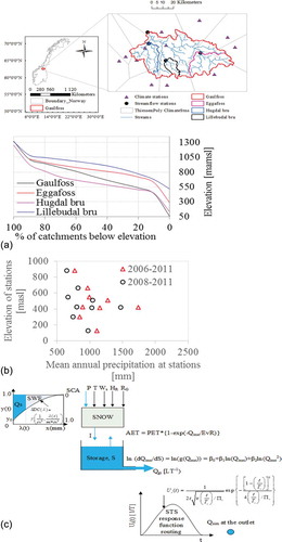
The climate data used are precipitation (P) from 12 stations, temperature (T) from 11 stations, wind speed (W_s) from 9 stations, and relative humidity (H_R) and global radiation (R_G) from 3 stations. All climate input data are in hourly time resolution. The spatial fields of precipitation and other climate data on the 1 × 1 km² grids were computed by inverse distance weighing (IDW). An average adiabatic temperature lapse rate of −0.65°C/100 m was considered in the spatial interpolation for temperature. The precipitation records from the stations used in the present study do not display any simple orographic precipitation gradients (elevation–precipitation relationship) for the region (Fig. 1b). This may be due to the fact that the complexities of precipitation patterns and dynamics in this mountain region cannot be captured adequately using the sparsely distributed precipitation gauging stations. Therefore, using elevation-based interpolation or accounting for precipitation gradients by incorporating a precipitation gradient parameter in the interpolation process would unreasonably modify the spatial precipitation fields and would force the model calibration to just a “fit-for purpose”. Therefore, the assumption is made that a basic IDW scheme may be applied for the purposes of this study, whilst recognizing its limitations.

3 Methods and models

3.1 Kirchner’s runoff response routine

Kirchner (2009) developed a runoff response routine (Fig. 1(c)) based on a water balance equation:

(1)

The water balance-based response routine is:

(2)

where the actual evapotranspiration (AET), infiltration (I), which is the sum of rainfall and snowmelt, discharge (Q) and bulk catchment storage (S) are given in mm; t is a time variable; G_in – G_out or the net groundwater flow across watershed boundary is assumed to be zero; g(Q) is as already defined; and β₀, β₁ and β₂ are regression parameters. The reciprocal of the sensitivity function, 1/g(Q), is the system “response time” or “memory” (Teuling et al. 2010), usually denoted as τ, and this indicates how rapidly streamflow recedes. Runoff was computed by solving the integral in Equation (2) in time using an adaptive Bogacki-Shampine (Bogacki and Shampine 1989) numerical method, implemented in ENKI (Kolberg and Bruland 2012). Observed discharge before the start of simulation period was used as the initial state for all grid cells to infer the initial storage.

In the lumped water balance model of Kirchner (2009), I, AET, Q and S in the above equations are lumped on the catchment scale. But in the present study we simulated distributed runoff for each grid cell by considering spatially distributed climate inputs, fluxes and storage. The grid-based computations account for the spatial variability of climate forcings. However, the model parameters, which are estimated from the recession analysis or calibrated in the present study, are “effective” parameters applied to all grid cells in the catchment. In the following two sections, we explain procedures for estimation of the regression parameters, i.e. runoff response parameters from streamflow recession analysis and parameter tuning by a calibration algorithm.

3.1.1 Estimation of the regression parameters and g(Q) from streamflow recession

The regression or runoff response parameters (β₀, β₁ and β₂) were estimated from recession analysis of observed streamflow. In this approach, the storage discharge characteristics of a catchment are inferred from measured fluctuations in discharge, particularly during winter recession periods in which evapotranspiration rates are expected to be small (Beven 2012). Recession plots provide information on how the rate of streamflow recession (−dQ/dt) varies with discharge (Q) when the effects of evapotranspiration and precipitation or infiltration are assumed negligible and hence Equation (2) for dQ/dt can be reduced to Equation (3):

(3)

The main advantages of recession analysis are that rainfall can be assumed to be zero, or at least small (so difficulties with any errors in catchment rainfall estimation are avoided), and that the hydrograph represents an aggregate measure of catchment behaviour (Sivapalan et al. 2003).

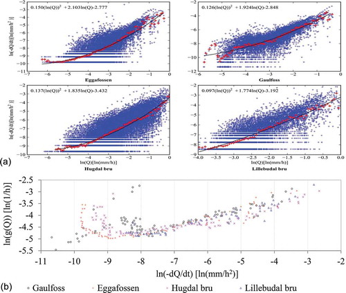
The refined recession analysis (extraction and binning) procedure by Kirchner (2009) was followed. For estimation of g(Q) from the recession analysis, we estimated the regression parameters based on bin-averaged discharges extracted from streamflow recessions. In this method, we used long time series of hourly data (1995–2011 for Gaulfoss, Eggafoss and Hugdal bru, and 2004–2011 for Lillebudal bru). We extracted only night-time recessions to avoid marked effects of evapotranspiration on estimation of regression parameters due to the assumptions of I ≪ Q and AET ≪ Q during the recession periods of the runoff hydrograph. However, we did not exclude periods with any marked precipitation compared to discharge due to lack of long hourly series of precipitation data. From the recession plots of observed streamflow (Fig. 2 (a)), we fitted a second-order polynomial between ln(−dQ/dt) and ln(Q). Rearranging for g(Q) in Equation (3), with log-transformation for numerical stability following Kirchner (2009), the following polynomial regression-based storage–discharge relationship was fitted from the recession analysis:

(4)

Figure 2. (a) Flow recession rates and fitted recession plots; (b) ln(−dQ/dt) versus ln(g(Q)) plots showing effects of the lower end of the recession.

where β₀, β₁ and β₂ are parameters of the polynomial regression model. The rate of flow recession (−dQ/dt) is computed as the difference in discharge between two successive hours, and the discharge Q is computed as average discharge over the two successive hours, following Brutsaert and Nieber (1977) and Kirchner (2009). We estimated the regression parameters using an ordinary least squares method:

(5)

where ԑ is an error term, Q_i represents bin-averaged discharges, n_b is the number of bin- averaged discharges.

However, the validity of the results depends on the adequacy of the fitted regression model. Hence, we tested the adequacy of the selected polynomial regression model. We diagnosed the multicollinearity, significance of the regression model and parameters, key features of residuals and parameter identifiability for the regression model. Though a polynomial regression with only two parameters obtained by setting the quadratic term β₂ = 0 may reduce problems related to correlation among the parameters, the regression model may not remain significant due to the lack of fit due to the missing quadratic term. We performed a significance test for the regression parameters and the regression model using the t-test and the F-test. We diagnosed the residuals for the normality assumption of the linear regression model by the Z-score test, which is the inverse of the standard normal distribution corresponding to a probability (p_r). The probability is given as p_r = (i − 0.5)/N, where i is the rank of the residuals in ascending order and N is the number of samples. We carried out diagnosis of residuals for homoscedasticity, correlation, systematic lack of fit and outliers from plots of the estimates of the response variable ln(g(Q)) versus the residuals, which should be random plots around an expected value of zero.

We estimated the individual confidence levels (ICL) for the parameters from the t-test. To assess identifiability of regression parameters through their joint confidence regions, we chose to compute the joint confidence region (JCR), which simultaneously bounds the joint parameters, to assess the effects of parameter correlation based on elliptical confidence regions (Bard 1974). Elliptical joint confidence regions are better predictors of regression model uncertainty because they capture the parameter correlation (Rooney and Biegler 2001). From the multivariate normal distribution of regression parameters given in Appendix A, the sum of squares function in the exponent term of Equation (A1) is the equation of a hyper-ellipse centred at the parameter estimates. The joint confidence region is all the points in the ellipsoid region and computed from the F-distribution as:

(6)

where θ is the subset of β that denotes the regression parameters in Equation (6), C is the part of the (X^TX)⁻¹ matrix corresponding to the parameters for which the joint confidence region is to be constructed, p' < p is the dimension of the parameters for which the joint confidence region is to be constructed, and the underline denotes a matrix or a vector. In the present study p' = 2, since we computed the joint confidence regions of two parameters at a time. α is the significance level, S² is estimated error variance = SSE/(N − p), where p denotes the number of parameters. Equation (6) is exact for the linear regression model (Rooney and Biegler 2001, Vugrin et al. 2007).

3.1.2 Model parameters and g(Q) from direct calibration

In this case, the regression parameters (Equation 4) along with other model parameters (Table 2) were calibrated based on precipitation–streamflow relationships to compute g(Q). The differential evolution adaptive Metropolis algorithm or DREAM (Vrugt et al. 2009) with a residual-based log-likelihood objective function implemented in the ENKI hydrological modelling framework (Kolberg and Bruland 2012) was used:

(7)

Table 2. Parameters and their prior ranges.

No.	Calibrated (free) parameter	Description	Unit	Prior range [Min., Max.]
	Snow
1	TX	Threshold temperature	°C	[−3,2]
2	WS	Snow melt sensitivity to wind speed	–	[1,6]
	Runoff response
3	EvR	Discharge at which AET equals 0.95PET	mm/h	[0.1,Qmax]
4	β0	Regression parameter (constant term)	–	[−4.2,−1]
5	β1	Regression parameter (linear term)	–	[0.2,1.5]
6	β2	Regression parameter (quadratic term)	–	[−0.5,0.5]
	Routing
7	V	Velocity of flow	m/s	[1.9,2.6]
8	D	Dispersion coefficient of flow	m^2/s	[200,1500]

Q_max is maximum streamflow for the calibration period.

where Q_sim^(λ) and Q_obs^(λ) are, respectively, Box-Cox (Box and Cox 1964) transformed simulated and observed streamflow series of length n, δ denotes model parameter, l denotes likelihood, λ is the Box-Cox transformation parameter and σ_ε² is variance of error. We computed λ from observed streamflow records based on the “fminsearch” algorithm in matlab, which finds the λ value that maximizes a log-likelihood function (http://www.mathworks.com). f_r is the fraction of effectively independent observations estimated from the autoregressive or AR(1) model of error covariance (Ziḙba 2010).

We used a 3-year (2007–2010) and a 1-year (2010–2011) hourly time series for parameter calibration and temporal validation, respectively, due to availability of only limited length climate data. We started the simulation in September and provided a sufficient “burn-in” period before the calibration period to reduce the effects of the initial snow state. We used the parameter set yielding maximum Nash-Sutcliffe efficiency (Nash and Sutcliffe 1970), denoted as NSE, for further analyses since it is a suitable and commonly used metric for comparison of streamflow hydrographs. We evaluated the simulation based on streamflow hydrographs and duration curves. Hydrographs are catchment-integrated signatures explaining how catchments respond to climate forcing and its own states. Flow duration curves express the temporal variability of flow in terms of the percentage of time a flow of a certain magnitude is available within a year. We tested the temporal transferability of both the estimated and calibrated parameters for the Gaulfoss catchment (3090 km²) and spatial transferability (validation) to internal sub-catchments of Eggafoss (653 km²), Hugdal bru (549 km²) and Lillebudal bru (168 km²). Uncertainty and identifiability of the calibrated parameters were assessed from the last 50% of the marginal posterior parameters obtained from the DREAM calibration algorithm.

3.2 Snow routine

Snow processes are dominant in the study area during winter and spring. Therefore, we used the gamma-distributed snow depletion curve-based routine (Kolberg and Gottschalk 2006) to compute the snow accumulation and meltwater release from saturated snow. The calibrated parameters in the snow routine are rainfall–snowfall threshold temperature (TX) and snowmelt sensitivity to wind speed (WS).

3.3 Evapotranspiration routine

In the present study, we computed the potential evapotranspiration, PET (mm/h) by the Priestley-Taylor method (Priestley and Taylor 1972):

(8)

where α is the Priestley-Taylor constant, ∆ is the slope of the saturation vapour pressure curve at air temperature at 2 m (kPa/°C), γ is the psychrometric constant (0.066 kPa/°C), R_n (W/m²) is net radiation, which is the sum of net shortwave radiation (SR_n) and net longwave radiation (LR_n), G is ground heat flux, L_v (kJ/m³) is volumetric latent heat of vaporization or energy required per water volume vaporized and Δt (s) is the simulation time step. We computed SR_n from the global radiation (R_G) and land albedo, and LR_n based on Sicart et al. (2006). We used α = 1.26, following Teuling et al. (2010), to reduce the number of calibrated parameters. The AET was computed from the PET and streamflow based on an evaporation ratio (EvR), which is a calibrated parameter. EvR represents the discharge at which AET equals 0.95PET (Fig. 1(c)). The streamflow was used as a proxy to indicate the soil-moisture state according to the equation given in Figure 1(c).

3.4 Runoff routing routine

Travel time lag influences the hydrological behaviour of large basins. To investigate the effects of runoff delay, we conducted calibration of parameters with and without the runoff routing routine. For runoff routing, we linked a response function-based source-to-sink (STS) routing (Naden 1992, Olivera 1996) to the recession-based model to account for the effects of runoff delay in both hillslopes and river networks. The runoff response at the outlet for the runoff signal at each grid cell i (i.e. spatially distributed) is given by the response function U_i(t) [T⁻¹], which is based on a travel time distribution and formulated as below (Olivera 1996, Hailegeorgis et al. 2015):

(9)

where Π_i [-] = Σ(l_iV_i/D_i) is the flow path Peclet number, T_i is expected flow travel time to the outlet for the grid cell i, t is a time variable and l_i is flow travel length in grid cell i. D_i (flow dispersion coefficient) and V_i (velocity of flow) are effective calibrated parameters used for all grid cells. We performed the runoff routing by a convolution following Maidment et al. (1996):

(10)

where Q_sim [L/T] is catchment-averaged routed simulated flow at the time step t, A_i [L²] is area of grid cell, A [L²] is catchment area, Q_gi [L/T] is average runoff (over time step) generated at each grid cell i and is the convolution operator.

4 Results

4.1 Recession plots and estimated g(Q)

Kirchner (2009) discussed the importance of measuring g(Q) across nested networks to understand how storage–discharge relationships vary across the landscape. For the four catchments in the present study, flow recession rates and recession plots or recession relationships fitted to bin-averaged discharges with their corresponding polynomial regression equations are given in Figure 2. The rate of streamflow recession (−dQ/dt) is 0.0000–0.031 mm/h² for Gaulfoss, 0.000055–0.0359 mm/h² for Eggafoss, 0.0000–0.0369 mm/h² for Hugdal bru and 0.00022–0.259 mm/h² for Lillebudal bru. The “response time” τ is 16–237 h for Gaulfoss, 19–145 h for Eggafoss, 22–126 h for Hugdal bru and 15–131 h for Lillebudal bru. The corresponding bin-averaged discharges (Q) are 0.0032–0.698 mm/h for Gaulfoss, 0.0020–0.744 mm/h for Eggafoss, 0.00298–0.948 mm/h for Hugdal bru and 0.0189–0.942 mm/h for Lillebudal bru. Response time (τ) is dependent on catchment size, i.e. the effects of runoff delay. The larger Gaulfoss catchment exhibits a slow response time while the smaller Hugdal bru and Lillebudal bru catchments exhibit fast response times. Storage characteristics of catchments also affect response time. Catchments with a slow recession rate are typically groundwater dominated, while impermeable catchments with little storage show faster recession rates (Staudinger et al. 2011).

4.2 Hydrographs and flow duration curves

We present simulated versus observed streamflow hydrographs of Gaulfoss for calibration and validation periods in Figure 3. Figure 3(a) corresponds to the regression parameters estimated from recession (with snow, evapotranspiration and runoff routing parameters from calibration), Figure 3(b) corresponds to calibrated parameters (runoff routed) and Figure 3(c) corresponds to calibrated parameters (runoff unrouted). Parameter estimation from recession and calibration (optimization) resulted in NSE of up to 0.77 and 0.82, respectively, and the model reproduced the hydrographs for Gaulfoss (Table 5). In addition, temporal transfer of parameters to the Gaulfoss catchment and spatial transfer of parameters to internal sub-catchments (Eggafoss, Hugdal bru and Lillebudal bru) based, respectively, on the “split sample” and “proxy basin” tests (Klemeś 1986) provided NSE values up to 0.81 for parameter estimation and 0.83 for calibration (Table 5). This also shows that the g(Q) computed from parameters estimated from recession segments and from calibration based on continuous streamflow observations both provide representative parameters to capture seasonal variations of streamflow hydrographs. However, parameter estimation from recession analysis and calibration without runoff routing both underestimate the peak flows compared to simulation based on calibration with runoff routing included. Figure 5(a) displays plots of observed versus simulated flow duration curves from combined calibration and validation periods. The model reproduced the temporal variability of streamflow in terms of the flow duration curve.

Table 3. Estimated and calibrated parameters corresponding to NSE for Gaulfoss.

Cases	TX	WS	EvR	β2	β1	β0	V	D
1	NSE: regression parameters estimated from recession*
	−1.482	5.708	0.273	0.130	0.920	−2.850	2.198	774.215
2	NSE: calibrated parameters (routed)
	−1.482	5.708	0.273	−0.040	0.684	−2.477	2.198	774.215
	NSE: calibrated parameters (unrouted)
3	−0.999	5.895	0.670	−0.127	0.286	−3.234

*Parameters other than the regression parameters are calibrated parameters for the runoff routed case. Bold font indicates regression parameters.

Table 4. Parameter correlation matrix (r), and maximum and minimum values of marginal posterior parameters from calibration (runoff-routed) for Gaulfoss.

Parameter	TX	WS	EvR	β1	β0	β2	V	D
TX	1.00	0.44	0.27	0.03	0.12	−0.07	0.06	0.05
WS		1.00	0.23	0.25	0.27	0.23	−0.28	0.12
EvR			1.00	0.51	0.64	0.40	−0.17	−0.37
β1				1.00	0.91	0.97	−0.28	−0.23
β0					1.00	0.80	−0.36	−0.23
β2						1.00	−0.23	−0.20
V							1.00	−0.08
D								1.00
Max.	−0.73	6.00	0.34	1.49	−1.55	0.10	2.59	1466.24
Min.	−1.41	2.71	0.13	0.27	−3.63	−0.13	1.91	201.11

Bold font indicates |r| > 0.6.

Table 5. Results for maximum values of NSE for parameter estimation from recession segments and calibration for Gaulfoss, and temporal and spatial transferability or validation for “proxy ungauged” internal sub-catchments.

Cases	Max. NSE	Temporal validation (01/09/2010–01/09/2011)	Spatial validation
			Eggafoss	Hugdal bru	Lillebudal bru
1	NSE: regression parameters estimated from recession
	0.77	0.81	0.70	0.80	0.55
2	NSE: calibrated parameters (runoff routed)
	0.82	0.83	0.68	0.75	0.52
3	NSE: calibrated parameters (runoff unrouted)
	0.80	0.82	0.65	0.79	0.51

Figure 3. Hydrographs for Gaulfoss corresponding to the NSE: (a) regression parameters estimated from recession (runoff routed); (b) calibrated parameters (runoff routed); and (c) calibrated parameters (runoff unrouted). Simulation for calibrated or estimated parameters (1 September 2008–1 September 2010) and simulation for temporal validation (1 September 2010–1 September 2011). P represents IDW interpolated and catchment averaged precipitation.

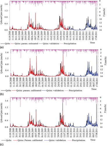
Figure 4. (a) Typical results from diagnostic of the regression for the recession analysis: normality test for Hugdal bru (left), residuals plot for Gaulfoss (middle) and systematic lack of fit due to missing quadratic term for Eggafoss (right); (b) 95% ICL and JCR for regression parameters for Gaulfoss; (c) parameter uncertainty in terms of histograms of marginal posteriors from calibration (runoff-routed) for Gaulfoss.

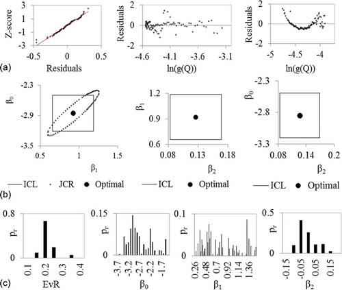
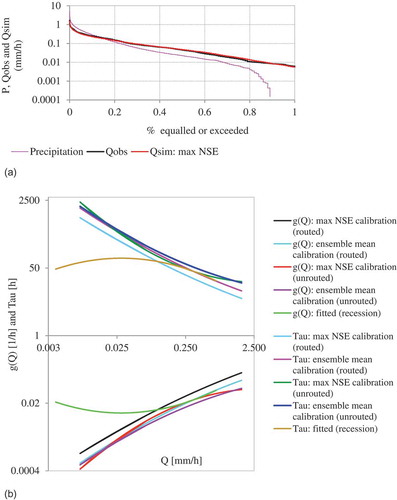
Figure 5. (a) Precipitation and streamflow duration curves and (b) discharge sensitivity function (g(Q)) and “response time” (τ) for Gaulfoss. The g(Q) and τ were computed based on Equation (4) from the regression parameters estimated or obtained by calibration.

4.3 Parameter uncertainty and identifiability

Table 2 lists calibrated parameters along with their ranges of prior values, whereas Table 3 gives values of the parameters estimated and calibrated for both runoff routed and unrouted cases corresponding to the maximum NSE for the Gaulfoss catchment. Figures 4(a) and (b) show, respectively, typical results from diagnostics of the polynomial regression and uncertainty bounds of regression parameters for parameter estimation from streamflow recession. Figure 4(c) presents uncertainty of the calibrated response routine parameters (runoff routed) in terms of histograms of marginal posterior distributions from calibration. The parameters β₀ and β₁ exhibit wider posterior distributions (large uncertainty) compared to β₂ and EvR.

Diagnostics of the fitted second-order polynomial regression of the recession analysis reveal the adequacy of the model. The parameters and the model are significant, and normality and randomness of the residuals comply with the key assumptions in the regression model. However, the residual plots show systematic lack of fit, indicating that the regression model appears to be not significant for some of the study catchments when there is no quadratic term.

The rectangular region created by individual 95% confidence limits based on the t-test indicates wide uncertainty ranges. We performed tests on whether it is necessary to consider the joint confidence regions to account for the correlation among the regression parameters for the Gaulfoss catchment. The majority of ellipsoid joint confidence regions lie inside the rectangular individual confidence limits for β₀ and β₁ (Fig. 4(b)), which indicates that considering joint confidence regions is not necessary for these parameters. However, the elliptical joint confidence regions involving the quadratic parameter β₂ (not shown here) are far from their corresponding rectangular individual confidence limits, which indicates poor identifiability due to correlation between the parameters, and hence suggests removing the quadratic term containing β₂ from the regression model.

However, significance tests based on residuals analyses (Fig. 4(a)) reveal that the regression model is not adequate for some cases without the quadratic term, as discussed earlier. Despite these two contradictory results, we preferred to use the second-order polynomial regression with the three parameters (constant, linear and quadratic terms) of Equation (5) in the present study. Even though the regression parameters estimated from recession analysis are different from the optimized values (Table 3), their uncertainty bounds somehow overlap. This can be observed by comparing the confidence limits or regions (Fig. 4(b)) versus histograms of posterior parameters for the Gaulfoss catchment (Fig. 4(c)).

Table 4 shows the results of parameter correlation in terms of the linear correlation matrix and ranges of posterior parameters for the Gaulfoss catchment. The large linear correlations among the response routine parameters for the direct calibration indicate poor identifiability of parameters. To address the effects of parameter uncertainty on g(Q), Figure 5(b) presents the effects of parameter estimation, parameter calibration and runoff delay on g(Q) along with the ensemble mean of g(Q) computed from posterior parameter sets from the calibration.

4.4 Parameter transferability

The transferability of model parameters from Gaulfoss (3090 km²) to its three internal sub-catchments, Eggafoss (653 km²), Hugdal bru (549 km²) and Lillebudal bru (168 km²), shows the validity of the “top-down” modelling approach. However, the performance of parameter transfer to Lillebudal is lower than that of the others.

5 Discussion

5.1 Model calibration and validation

The results from the present study indicate that the principle of “catchments as simple dynamical systems”, in which the streamflow is assumed to be controlled mainly by the release of water from the storage, provides reasonable runoff simulation for a catchment dominated by boreal glacial tills. Though the occurrence of preferential flow in glacial till soil has been reported (e.g. Jansson et al. 2005), the present study shows that streamflow simulation based on the main assumption of hydraulic connectivity of storage and flow pathways provided satisfactory calibration and validation results. Both the parameters estimated from streamflow recession and calibrated parameters could represent effective characteristics of the heterogeneous catchment system (see Beven et al. 2000, Wagener and Wheater 2006). Calibrated effective parameters are assumed to take into account all the local-scale heterogeneity of land surface characteristics, meteorological variables and hydrological processes and fluxes for large areas (Gottschalk et al. 2001, Beldring et al. 2003).

However, both parameter estimation from recession segments and direct calibration of precipitation–runoff relationships without considering the effects of runoff routing slightly underestimate the peak flows compared to parameter calibration with runoff routing included. This result does not agree with that of Brauer et al. (2013), who found that for a less-humid catchment in The Netherlands parameter calibration for a power-law storage–discharge relationship led to strong underestimation of the response of runoff to rainfall, while parameter estimation from recession analysis lead to an overestimation. The discrepancy may arise due to the difference between the polynomial relationship derived from the recession analysis in this study and the pre-determined power-law relationship in Brauer et al. (2013), and the differences in the calibration and the runoff routing algorithms.

5.2 Transferability of model parameters

The results of the model were spatially validated based on the transferability of model parameters from the Gaulfoss catchment to internal sub-catchments, which indicates an opportunity for transfer of parameters to ungauged sites in the catchment. Kirchner (2009) noted that if g(Q) can be estimated from some combination of catchment characteristics, then it may help in solving the problem of hydrological prediction in ungauged basins. This would also allow distributed parameterization of the regression parameters. However, a previous attempt by Krakauer and Temimi (2011) to identify first-order controls of recession time scale indicated that the predictor variables were significant only at high or low flow rates. Moreover, observations of the geological characteristics of the catchments, which influence the recession behaviour, are not readily available and there are limitations associated with the data mining or spatial analysis methods. In addition, Pokhrel et al. (2008) and Pokhrel and Gupta (2011) illustrated the limitations of making inferences on the spatial properties of a distributed model when only information about catchment output stream response is available. Nevertheless, the temporal and spatial transferability of the estimated and calibrated model parameters substantiate further evaluation of parameter transferability on a larger number of catchments.

5.3 Effects of parameter uncertainty on the g(Q)

Parameter uncertainty affects the discharge sensitivity to storage, g(Q), and hence streamflow simulation. We found considerable differences between the values of g(Q) computed from estimated and calibrated parameters for the Gaulfoss catchment (Fig. 5(b)). For the recession-based analysis, g(Q) was found to be an increasing function of Q only above certain limits of Q. A problem is associated with the lower ends of the recession segments. Kirchner (2009) discussed the significant scatter at the lower end of the recession, particularly for Q < 0.1 mm/h and attributed it to the effects of measurement noise. As we can observe from the lower ranges of recession rates in Figure 2(a), there are equal recession rates over the ranges of bin-averaged discharges. The ln(−dQ/dt) versus ln(g(Q)) plot in Figure 2(b) also shows higher observed g(Q) for the lower ends of the recession plots, which may not be related to fluctuations in catchment storage, but rather may be related to the resolution of loggers and errors in measurements of low winter flows. These figures suggest cutting off the lower end of the recession below ln(−dQ/dt) < −8.0 or below ln(Q) < −3.20 for Gaulfoss, and similarly for the other catchments.

However, the values of the estimated parameters are sensitive to the cut limits of the lower end of the recession. We obtained markedly different recession parameters from different cut limits of the lower ends of recession curves. Moreover, the estimated parameter sets based on different lower cut limits provided equivalently good performances of runoff simulation, which obviously indicates a major source of uncertainty. Therefore, in the present study we kept the lower ends of the recession segments while estimating the parameters. Instead, we limited the upper end of the recession to ln(Q) = 0 to remove outliers above this limit, which are most probably attributable to the errors in streamflow measurements during high-flow recessions. Further study is required to address uncertainties due to the lower end of the recession and other sources in a comprehensive manner, which was not the main objective of this study. Stoelzle et al. (2012) compared different recession extraction and fitting procedures and found considerable differences in the results. Differences between the g(Q) found from recession analysis and direct calibration may also arise since the g(Q) from recession analysis was obtained from parameter estimation based on only night-time hourly streamflow recessions for 17 years of data, while the g(Q) from calibration was based on 2 years of hourly continuous records. While estimation of g(Q) from the long records allows consideration of the temporal variability of flows, continuous records in the case of calibration allow inclusion of all ranges of streamflow, which have different degrees of sensitivity to the storage.

We also found that incorporating shorter recession segments in the analysis provided a nearly constant τ and g(Q). Since streamflow fluctuations causing recessions only for short periods may not be related to catchment storage, we set a minimum length of recession segments to include in the analysis to exclude the shorter discharge fluctuations. Selection of recession segments longer than 9–15 hr provided nearly similar patterns of g(Q) for Gaulfoss and Eggafoss and hence we extracted recession segments of ≥9 hr for the two catchments and ≥4 hr for Hugdal bru and Lillebudal bru.

The differences in parameters estimated from recession segments versus those obtained by calibration, and the differences in calibrated parameters with runoff routing and without runoff routing are observed in both the slope and the intercept parameters (Table 3). It is difficult to distinguish the effects of the procedures of the recession analysis from the effects of runoff delay related to river networks or catchment size. However, model calibration allows quantification of uncertainty in the g(Q) from the posterior parameters. The ensemble means of g(Q) obtained from the last 1000 posterior parameters sets are lower than the g(Q) corresponding to the optimal parameter sets for both routed and unrouted runoff; the difference is more exaggerated for the routed runoff case (Fig. 5(b)).

5.4 Effects of catchment size (runoff delay) on simulation of peak flows

We obtained a maximum runoff delay or travel time lag between headwater and outlet of 14.81 hr for the Gaulfoss catchment from calibration of parameters. While considering the runoff routing explicitly during the calibration, the routing parameters account for runoff delays in the hillslopes and channel networks and hence it is expected that the regression parameters of the runoff response routine do not compensate for the runoff delay. Therefore, in considering the runoff delay by calibrating the runoff routing parameters, we obtained a lower “response time” (τ = 1/g(Q)) compared to the case when runoff is unrouted (Fig. 5(b)). Despite the significant runoff travel time lag in the Gaulfoss catchment compared to the hourly runoff simulation, we found a slight underestimation of peak flows due to the effects of neglecting runoff routing during the calibration (Fig. 3(c)). In addition, there is no significant deterioration in the performance measure (NSE) due to neglecting the runoff delay. These results show that interaction or compensation among model parameters during calibration partially conceals the sensitivity of the outlet hydrographs to the effect of runoff delay, which is a problem related to parameter identifiability. Generally, the importance of runoff routing decreases with the catchment size and is almost negligible for the smallest modelled catchment of Lillebudal bru (Table 5).

5.5 Effects of sparsity of climate stations

Climate stations are available only inside the Gaulfoss and Hugdal bru catchments and hence more representative climate input is expected for these catchments than for Eggafoss and Lillebudal bru. In addition, a marked proportion of the Lillebudal catchment is located above the highest gauging station of 885 m a.m.s.l. (Fig. 1(a)) and hence precipitation records from low-lying areas may not represent the mountainous regions in the Lillebudal bru catchment. Therefore, computation of spatial precipitation fields from sparse precipitation stations may affect the parameter calibration and runoff simulation since the sparse gauging networks may not capture localized precipitation events. Orographic effects on precipitation may be pronounced in some mountainous regions. However, the available sparse climate data showed no defined orographic precipitation gradient in the region (Fig. 1(a)). Moreover, incorporating orographic effects in precipitation–runoff models requires extensive study, since orographic effects may vary between storms and years (e.g. Lundquist et al. 2010), the orographic precipitation gradient may reverse at a certain elevation threshold (e.g. Røhr and Killingtveit 2003), and leeward (rain-shadow) station records may not exhibit an orographic precipitation gradient (e.g. Nepal 2012). The spatially distributed climate input obtained from the IDW interpolation using point gauges from 3–12 stations is expected to provide a more reliable spatial distribution of precipitation and evaporation, which are the main inputs for the water balance model used in the present study, than does lumped modelling. However, dense climate stations that permit identification of precipitation and elevation relationships may improve the runoff simulation. Calibration based on data from high-density climate stations would also improve the uncertainty and non-identifiability of parameters for improved predictions using the recession-based model.

Slightly better transferability of parameters to internal sub-catchments for the parameter sets obtained from the recession analysis over the parameter sets obtained from the direct calibration (Table 5) may be attributable to the fact that parameter estimation from recession is dependent only on streamflow, while representativeness of climate input also affects the results of calibration.

6 Conclusions

The lumped recession-based “top-down” model suggested by Kirchner (2009) was adapted to a distributed simulation set-up, and augmented by snow accumulation and melt, and runoff routing models. The model provided acceptable calibration and validation results for the study catchments. Therefore, the results encourage further evaluation of the recession-based water balance model compared to other competing model structures on more catchments.

The lower end of the recession and the minimum length of recession segments included in the analysis were found to be the main sources of uncertainty for parameter estimation, which needs careful assessment. In addition, owing to the basic assumption of I≪ Q during recessions, evaluation of the effects of some marked precipitation events during recessions is required for parameter estimation from recession segments. Though estimation of runoff response parameters from only recession segments is practically possible, it exhibited the limitations of underestimating peak flows. Hence, parameter tuning by calibration based on the whole range of a streamflow hydrograph is unavoidable for improved simulation of flood events. Incorporating the effects of runoff delay (runoff routing) in the recession-based model is also required for improved simulation of peak flows in large-scale catchments. Despite the small number of calibrated parameters, the calibration results showed that the recession-based “top-down” model is susceptible to parameter uncertainty and identifiability problems, like other “top-down” and “bottom-up” models. Interaction among the parameters during calibration has the potential to partially mask the sensitivity of calibration to the runoff delay even for the macroscale catchment modelled in the present study. However, further evaluation of the reliability of runoff simulations and inferences made from the recession approach is required for any catchment size, for instance based on multi-objective calibration by utilizing observed distributed variables in addition to the catchment-integrated streamflow.

Acknowledgements

We express our thanks to the Norwegian Meteorological Institute, StatKraft, TrønderEnergi and Bioforsk for the climate data, and the Norwegian Water Resources and Energy Directorate for the streamflow data used in the present study. We are grateful to the anonymous reviewers for their comments, which helped to improve the manuscript.

Disclosure statement

No potential conflict of interest was reported by the authors.

Additional information

Funding

This work was a part of the HydroPEAK hydrology PhD project (grant number 50043420), which was financed by the Centre for Environmental Design of Renewable Energy (CEDREN).

Appendix

The multivariate normal probability density function for the regression parameters can be written as:

(A1)

where is a matrix of exploratory variables, is a vector of parameters, p is the total number of parameters, || is the determinant of the covariance matrix of the parameter estimates, σ² is variance, the underline represents a vector or a matrix, T denotes transpose and the hat notation represents an estimate.

References

- Ajami, H., et al., 2011. Quantifying mountain block recharge by means of catchment-scale storage–discharge relationships. Water Resources Research, 47 (4). doi:10.1029/2010WR009598
- Aksoy, H. and Wittenberg, H., 2011. Nonlinear baseflow recession analysis in watersheds with intermittent streamflow. Hydrological Sciences Journal, 56 (2), 226–237. doi:10.1080/02626667.2011.553614
- Ambroise, B., Beven, K., and Freer, J., 1996. Toward a generalization of the TOPMODEL concepts: topographic indices of hydrological similarity. Water Resources Research, 32 (7), 2135–2145. doi:10.1029/95WR03716
- Bard, Y., 1974. Nonlinear parameter estimation. New York, NY: Academic Press.
- Beldring, S., 2002. Runoff generating processes in boreal forest environments with glacial tills. Nordic Hydrology, 33 (5), 347–372.
- Beldring, S., et al., 2003. Estimation of parameters in a distributed precipitation-runoff model for Norway. Hydrology and Earth System Sciences, 7 (3), 304–316. doi:10.5194/hess-7-304-2003
- Bergström, S., 1976. Development and application of a conceptual runoff model for Scandinavian catchments. Norrköping, SMHI Report RHO 7, 134 pp.
- Beven, K., 2012. Rainfall-runoff modeling. 2nd ed. Oxford: Wiley-Blackwell.
- Beven, K.J., 2000. Uniqueness of place and process representations in hydrological modelling. Hydrology and Earth System Sciences, 4 (2), 203–213. doi:10.5194/hess-4-203-2000
- Beven, K.J., 2006. Searching for the Holy Grail of scientific hydrology: Qt=(S, R, Δt)A as closure. Hydrology and Earth System Sciences, 10, 609–618. doi:10.5194/hess-10-609-2006
- Beven, K.J. and Binley, A.M., 1992. The future of distributed models: model calibration and uncertainty prediction. Hydrological Processes, 6, 279–298. doi:10.1002/(ISSN)1099-1085
- Beven, K.J., Freer, J., Hankin, B., and Schulz, K., 2000. The use of generalized likelihood measures for uncertainty estimation in higher-order models of environmental systems. In: Fitzgerald, Smith, R.C., Walden, A.T., & Young, P.C., eds. Nonlinear and nonstationary signal processing, UK: Cambridge University Press.
- Blöschl, G., 2006. Hydrologic synthesis: across processes, places, and scales. Water Resources Research, 42, W03S02. doi:10.1029/2005WR004319
- Bogacki, P. and Shampine, L.F., 1989. A 3 (2)pair of Runge–Kutta formulas. Applied Mathematics Letters, 2 (4), 321–325. doi:10.1016/0893-9659(89)90079-7
- Box, G.E.P. and Cox, D.R., 1964. An analysis of transformations. Journal of the Royal Statistical Society, Series B, 26, 211–252.
- Brauer, C.C., et al., 2013. Investigating storage–discharge relations in a lowland catchment using hydrograph fitting, recession analysis and soil moisture data. Water Resources Research, 49, 4257–4264. doi:10.1002/wrcr.20320
- Brutsaert, W. and Nieber, J.L., 1977. Regionalized drought flow hydrographs from a mature glaciated plateau. Water Resources Research, 13, 637–643. doi:10.1029/WR013i003p00637
- Clark, M.P., et al., 2009. Consistency between hydrological models and field observations: linking processes at the hillslope scale to hydrological responses at the watershed scale. Hydrological Processes, 23, 311–319. doi:10.1002/hyp.v23:2
- Cunderlik, J.M., et al., 2013. Integrating logistical and technical criteria into a multiteam, competitive watershed model ranking procedure. Journal of Hydrologic Engineering, 18, 641–654. doi:10.1061/(ASCE)HE.1943-5584.0000670
- Ewen, J. and Birkinshaw, S.J., 2007. Lumped hysteretic model for subsurface stormflow developed using downward approach. Hydrological Processes, 21 (11), 1496–1505. doi:10.1002/(ISSN)1099-1085
- Fiorotto, V. and Caroni, E., 2013. A new approach to master recession curve analysis. Hydrological Sciences Journal, 58 (5), 966–975. doi:10.1080/02626667.2013.788248
- Fovet, O., et al., 2015. Hydrological hysteresis and its value for assessing process consistency in catchment conceptual models. Hydrology and Earth System Sciences, 19, 105–123. doi:10.5194/hess-19-105-2015
- Gottschalk, L., et al., 2001. Regional/macroscale hydrological modelling: a Scandinavian experience. Hydrological Sciences Journal, 46 (6), 963–982. doi:10.1080/02626660109492889
- Hailegeorgis, T.T., et al., 2015. Evaluation of different parameterizations of the spatial heterogeneity of subsurface storage capacity for hourly runoff simulation in boreal mountainous watershed. Journal of Hydrology, 522, 522–533. doi:10.1016/j.jhydrol.2014.12.061
- Jansson, C., Espeby, B., and Jannson, P.-E., 2005. Preferential flow in glacial till soil. Hydrology Research, 36 (1), 1–11.
- Jarvis, P.G., 1993. Prospects for bottom-up models. In: J.R. Ehleringer and C.B. Field, eds. Scaling physiological processes: leaf to globe. New York: Academic Press.
- Kirchner, J.W., 2006. Getting the right answers for the right reasons: linking measurements, analyses, and models to advance the science of hydrology. Water Resources Research, 42, W03S04. doi:10.1029/2005WR004362
- Kirchner, J.W., 2009. Catchments as simple dynamical systems: catchment characterization, rainfall-runoff modeling, and doing hydrology backward. Water Resources Research, 45, W02429. doi:10.1029/2008WR006912
- Klemeš, V., 1986. Operational testing of hydrological simulation models. Hydrological Sciences Journal, 31, 13–24. doi:10.1080/02626668609491024
- Klemeš, V., 1983. Conceptualization and scale in hydrology. Journal of Hydrology, 65, 1–23. doi:10.1016/0022-1694(83)90208-1
- Kolberg, S.A. and Bruland, O., 2012. ENKI - an open source environmental modelling platform. Geophysics Research Abstracts, 14, EGU2012–13630. EGU General Assembly.
- Kolberg, S.A. and Gottschalk, L., 2006. Updating of snow depletion curve with remote sensing data. Hydrological Processes, 20 (11), 2363–2380. doi:10.1002/(ISSN)1099-1085
- Krakauer, N.Y. and Temimi, M., 2011. Stream recession curves and storage variability in small watersheds. Hydrology and Earth System Sciences, 15, 2377–2389. doi:10.5194/hess-15-2377-2011
- Krier, R., et al., 2012. Inferring catchment precipitation by doing hydrology backward: A test in 24 small and mesoscale catchments in Luxembourg. Water Resources Research, 48, W10525. doi:10.1029/2011WR010657
- Lamb, R. and Beven, K.J., 1997. Using interactive recession curve analysis to specify a general catchment storage model. Hydrology and Earth System Sciences, 1, 101–113. doi:10.5194/hess-1-101-1997
- Lambert, A.O., 1969. A comprehensive rainfall-runoff model for an upland catchment area. Journal of the Institute of Water Engineering, 23, 231–238.
- Lundquist, J.D., et al., 2010. Relationships between barrier jet heights, orographic precipitation gradients, and streamflow in the Northern Sierra Nevada. Journal of Hydrometeorology, 11, 1141–1156. doi:10.1175/2010JHM1264.1
- Maidment, D.R., et al., 1996. A unit hydrograph derived from a spatially distributed velocity field. Hydrological Processes, 10 (6), 831–844. doi:10.1002/(ISSN)1099-1085
- Martina, M.L.V., Todini, E., and Liu, Z., 2011. Preserving the dominant physical processes in a lumped hydrological model. Journal of Hydrology, 399, 121–131. doi:10.1016/j.jhydrol.2010.12.039
- McDonnell, J.J., et al., 2007. Moving beyond heterogeneity and process complexity: a new vision for watershed hydrology. Water Resources Research, 43, W07301. doi:10.1029/2006WR005467
- Moore, R.J., 1985. The probability-distributed principle and runoff production at point and basin scales. Hydrological Sciences Journal, 30, 273–297. doi:10.1080/02626668509490989
- Myrabo, S., 1997. Temporal and spatial scale of response area and groundwater variation in Till. Hydrological Processes, 11, 1861–1880. doi:10.1002/(SICI)1099-1085(199711)11:14<1861::AID-HYP535>3.0.CO;2-P
- Naden, P.S., 1992. Spatial variability in flood estimation for large catchments: the exploitation of channel network structure. Hydrological Sciences Journal, 37, 53–71. doi:10.1080/02626669209492561
- Nash, J.E. and Sutcliffe, J.V., 1970. River flow forecasting through conceptual models part I — A discussion of principles. Journal of Hydrology, 10, 282–290. doi:10.1016/0022-1694(70)90255-6
- Nepal, S., 2012. Evaluating upstream–downstream linkages of hydrological dynamics in the Himalayan region. Thesis (PhD). Friedrich Schiller University of Jena.
- Olivera, F., 1996. Spatially distributed modeling of storm runoff and nonpoint source pollution using geographic information systems, Thesis (PhD). Department of Civil Engineering, University of Texas at Austin, USA.
- Parajka, J. and Bloschl, G., 2008. The value of MODIS snow cover data in validating and calibrating conceptual hydrologic models. Journal of Hydrology, 358, 240–258. doi:10.1016/j.jhydrol.2008.06.006
- Pokhrel, P. and Gupta, H.V., 2011. On the ability to infer spatial catchment variability using streamflow hydrographs. Water Resources Research, 47, W08534. doi:10.1029/2010WR009873
- Pokhrel, P., Gupta, H.V., and Wagener, T., 2008. A spatial regularization approach to parameter estimation for a distributed watershed model. Water Resources Research, 44, W12419. doi:10.1029/2007WR006615
- Priestley, C.H.B. and Taylor, R.J., 1972. On the assessment of surface heat flux and evaporation using large-scale parameters. Monthly Weather Review, 100, 81–92. doi:10.1175/1520-0493(1972)100<0081:OTAOSH>2.3.CO;2
- Ragletti, S. and Pellicciotti, F., 2012. Calibration of a physically based, spatially distributed hydrological model in a glacierized basin: on the use of knowledge from glaciometeorological processes to constrain model parameters. Water Resources Research. 48. 10.1029/2011WR010559
- Rees, H.G., et al., 2004. Recession-based hydrological models for estimating low flows in ungauged catchments in the Himalayas. Hydrology and Earth System Sciences, 8 (5), 891–902. doi:10.5194/hess-8-891-2004
- Røhr, P.C. and Killingtveit, Å., 2003. Rainfall distribution on the slopes of Mt Kilimanjaro. Hydrological Sciences Journal, 48 (1), 65–77. doi:10.1623/hysj.48.1.65.43483
- Rooney, W.C. and Biegler, L.T., 2001. Design for model parameter uncertainty using nonlinear confidence regions. Process Systems Engineering, 47, 1794–1804.
- Sicart, J. E., et al., 2006. Incoming longwave radiation to melting snow: observations, sensitivity and estimation in northern environments. Hydrological Processes, 20, 3697–3708.
- Singh, V.P. and Woolhiser, D.A., 2002. Mathematical modeling of watershed hydrology. Journal of Hydrologic Engineering, 7, 270–292. doi:10.1061/(ASCE)1084-0699(2002)7:4(270)
- Sivapalan, M., et al., 2003. Downward approach to hydrological prediction. Hydrological Processes, 17, 2101–2111. doi:10.1002/hyp.v17:11
- Spence, C., et al., 2010. Storage dynamics and streamflow in a catchment with a variable contributing area. Hydrological Processes, 24, 2209–2221. doi:10.1002/hyp.7492
- Staudinger, M., et al., 2011. Comparison of hydrological model structures based on recession and low flow simulations. Hydrology and Earth System Sciences, 15, 3447–3459. doi:10.5194/hess-15-3447-2011
- Stoelzle, M., Stahl, K., and Weiler, M., 2012. Are streamflow recession characteristics really characteristic? Hydrology and Earth System Sciences Discussions, 9, 10563–10593. doi:10.5194/hessd-9-10563-2012
- Teuling, J., et al., 2010. Catchments as simple dynamical systems: experience from a Swiss prealpine catchment. Water Resources Research, 46, W10502. doi:10.1029/2009WR008777
- Vrugt, J.A., et al., 2009. Accelerating Markov Chain Monte Carlo simulation by differential evolution with self-adaptive randomized subspace sampling. Journal of Nonlinear Sciences and Numerical Simulation, 10 (3), 273–290.
- Vugrin, K.W., et al., 2007. Confidence region estimation techniques for nonlinear regression in groundwater flow: three case studies. Water Resources Research, 43, W03423. doi:10.1029/2005WR004804
- Wagener, T., et al., 2007. Catchment classification and hydrologic similarity. Geography Compass, 1, 901–931. doi:10.1111/j.1749-8198.2007.00039.x
- Wagener, T. and Wheater, H.S., 2006. Parameter estimation and regionalization for continuous rainfall-runoff models including uncertainty. Journal of Hydrology, 320, 132–154. doi:10.1016/j.jhydrol.2005.07.015
- Wittenberg, H. and Sivapalan, M., 1999. Watershed groundwater balance estimation using streamflow recession analysis and baseflow separation. Journal of Hydrology, 219, 20–33. doi:10.1016/S0022-1694(99)00040-2
- Zehe, E. and Sivapalan, M., 2009. Threshold behaviour in hydrological systems as (human) geo-ecosystems: manifestations, controls, implications. Hydrology and Earth System Sciences, 13, 1273–1297. doi:10.5194/hess-13-1273-2009
- Ziḙba, A., 2010. Effective number of observations and unbiased estimators of variance for autocorrelated data an overview. Metrology and Measurement Systems, XVII (1), 3–16. doi:10.2478/v10178-010-0001-0