Estimation of soil water content in watershed using artificial neural networks

ABSTRACT

Soil water content (SWC) is an important factor in transfer processes between soil and air, contributing to water and energy balances, and quantifying it remains a challenge. This study uses artificial neural networks (ANNs) to analyse spatial and temporal variation of SWC in a Brazilian watershed, based on climate information, soil physical properties and topographic variables. Thirty eight input variables were tested in 200 models. The outputs were compared with 650 gravimetric moisture measurements collected at 26 points (25 field studies). The results show that it is possible to estimate SWC efficiently (Nash-Sutcliffe statistic, NS = 0.77) using topographic data, soil physical properties and rainfall. If only climate information is considered, modelling is less efficient (NS = 0.28). Using many variables does not necessarily improve performance. Alternatively, SWC can be estimated by simplified models using rainfall and topographic maps information, although the performance is less good (NS = 0.65).

KEYWORDS:

• gravimetric moisture
• spatial and temporal distribution
• physical soil parameters
• artificial neural networks

Editor D. Koutsoyiannis; Associate editor F.-J. Chang

1 Introduction

Soil water content (SWC) is one of the determining factors in the transfer processes between soil and air, contributing directly to water and energy balances. It is essential knowledge for water resource management in several fields, including prevention of natural disasters such as landslides and floods, flow estimation by hydrological models with different objectives, estimation of sediment production, and studies of nutrient and pollutant transport in soil. SWC is strongly correlated with river flow and can be used to estimate it (Humphrey et al. 2016).

Spatial and temporal variability of SWC is scale dependent (Cantón et al. 2010) and controlled by complex interactions that involve variables related to rainfall (Famiglietti et al. 1998, Korres et al. 2013), soil (Famiglietti et al. 1998, Vereecken et al. 2007, Wang et al. 2012, Hu and Si 2014, Zhang and Shao 2015), vegetation (Baroni et al. 2013, Zhang and Shao 2015), topography (Famiglietti et al. 1998, Zhu and Lin 2011, Wang et al. 2012, Sur et al. 2013, Zhang and Shao 2015) and climate (Western et al. 2004, Wang et al. 2012, Cho and Choi 2014). The importance of each of these variables depends on the predominant characteristics of the site analysed (Western et al. 2004) and the behaviour of many of them is influenced by the presence of the others, making it difficult to identify their cause and effect relations that determine SWC (Korres et al. 2013). This relatively complex pattern of SWC distribution (Van Oevelen 1998) requires high spatial and temporal density of observations and makes it difficult to estimate this content adequately on a spatio-temporal scale (Western et al. 2002, Vereecken et al. 2007).

Currently, SWC can be estimated by point measurements at points in a watershed, or by remote sensing techniques (Western et al. 2002). The former can also be classified as direct methods (collection of soil samples) or indirect methods (measurements by tensiometers, neutron probes, electrical capacitance sensors, electrical resistance sensors, heat dissipation sensors and temporal domain reflectometers – TDR or frequency). Using indirect methods, it is possible to estimate the SWC through its relationship with other measurable variables (Dobriyal et al. 2012, Muñoz-Carpena 2012), usually a physical or physicochemical property related to SWC (Romano 2014), by constructing a calibration curve to describe the relation between them (Köksal et al. 2011).

Among the approaches available, point measurements in soil, whether manual or automatic, are the simplest and most precise (Western et al. 2002). However, whatever method is used, considerable resources and time are required, and the information obtained is limited to a few selected points.

Remote sensing techniques are effective to estimate SWC in time over large areas, with good results (Chai et al. 2010, Paloscia et al. 2013). However, this technology is still relatively expensive and complex (Dobriyal et al. 2012), and is subject to a number of limitations, including limited spatial resolution (affecting mainly small basins) and difficulties in interpreting the signal, especially because of the influence of surface roughness, effects of distortions caused by topography, uncertainties regarding the relationship between the sensor responses and SWCs (Wang and Qu 2009), and the difficulty of identifying the variations of these responses when there is vegetation (Western et al. 2004). In this case it may also be necessary to take field measurements to validate model estimates. Moreover, it is not possible to obtain SWC from a single satellite image; it being necessary to use images on various dates corresponding to the collection campaigns.

Because of these difficulties, some authors have recently used artificial neural networks (ANNs) to estimate SWC, stimulated mainly by the success of applying such networks to solve many complex and nonlinear problems in widely different fields. Most of them estimate SWC from parameters obtained by satellite or radar images such as surface brightness, temperature, vegetation index and backscattering coefficient (Paloscia et al. 2008, 2013, Said et al. 2008, Chai et al. 2010, Santi et al. 2012, Srivastava et al. 2013, Cui et al. 2016, Hassan-Esfahani et al. 2017). Some use at least one climate variable, often precipitation, temperature, air humidity, grass temperature and solar radiation. (Contador et al. 2006, Elshorbagy and Parasuraman 2008, Ramírez-Beltran et al. 2008, Coelho et al. 2009, Mustafa 2016). Some have also used information about the soil, including clay content and density (Ramírez-Beltran et al. 2008, Zou et al. 2010, Köksal et al. 2011, Arsoy et al. 2013), and about topography, including curvature, and topographic index of the study area (Contador et al. 2006). Fashi (2016) estimated soil saturation percentage of flood areas in Iran with ANNs and obtained promising results.

Artificial neural networks are statistical and empirical models that have a good capacity to adapt, learn and generalize (Kröse and Smagt 1996, Kasabov 1998), and they are considered promising tools for environmental modelling. In addition, they have a good ability to separate and organize data (Kröse and Smagt 1996), robustness, great parallelism, associative storage of information and its spatio-temporal processing (Kasabov 1998). However, one problem when using ANNs is the impossibility of predicting inputs and outputs that are outside the network training limits (ASCE 2000), and therefore it is essential to have adequate sampling data available for training.

The aim of the research reported here was to develop a method for estimating SWC, based on information about climate, soil physical properties and watershed topographical variables, using simulation by ANNs. The search for the best model predictor will also provide clarification on which variables have the greatest influence on SWC, contributing to the choice of variables to be monitored in pedotransfer research to estimate SWC. Furthermore, since the model is efficient, it will provide an estimate of SWC at any point of the basin that has not been sampled and for periods before and after the periods monitored, provided that the variables are within the domains used for model training.

It is intended to apply the resulting models to SWC estimation in homogeneous physico-climatic regions of the area studied, within the domains of input variables and output variable from which the ANN was constructed. However, even in different physico-climatic regions it is also possible to use the same methodology developed in this study to obtain analogous models, but including other important variables for a region that describe its geology and soil characteristics.

2 Artificial neural networks

In many hydrological applications, a multiple layer perceptron (MLP) type of ANN is commonly used, with a three-layer structure (Singh and Frevert 2006). This network (Fig. 1) is a universal approximator (Hornik et al. 1989), and is characterized by (i) an input layer, one (or more) intermediate layers and one output layer; and (ii) connections with their associated (synaptic) weights, analogous to natural networks, between neurons in one layer and the layer that follows it. The number of intermediate layers, and the number of neurons in each such layer, are generally determined by trial and error.

Figure 1. Neural network with multiple layers (adapted from Matos et al. 2014).

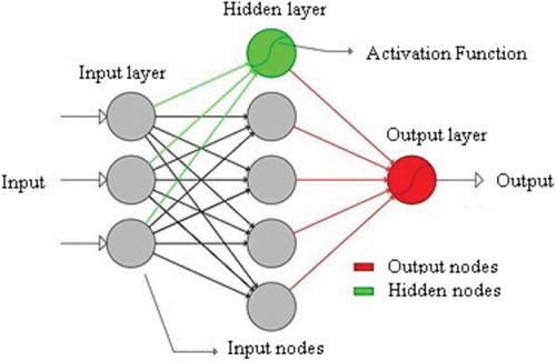
Each neuron receives the sum of the inputs from neurons leading into it, weighted using the respective synaptic weights; this sum then undergoes a transformation, generally nonlinear, known as the neuron activation function. Neuron function is defined by:

(1)

where O is the neuron response value; f is the activation function; w_i are the synaptic weights; I_i are the values of the n inputs that will be processed in the neuron; and b is the tendency or bias.

The most widely used form for the activation function is the unipolar sigmoid function, because of the simplicity of its derivative (Fantín-Cruz et al. 2011, Oliveira et al. 2013). Equation (2) shows the format of the unipolar sigmoid function and Equation (3) represents the derivative of this function:

(2)

(3)

where η is the net input of the neuron, defined as the result of w_iI_i + b.

The synaptic weights of the connections are adjusted by training the network, by means of a learning rule; they are adjusted by minimizing a measure of the errors between output from the network and the observed output.

The training method most widely used is the back-propagation algorithm (Rumelhart et al. 1986), which is a generalization of the Delta Rule proposed by Widrow and Hoff (1960). This consists of searching, on the performance surface, for a minimum point of the quadratic error function, according to (Widrow and Hoff 1960):

(4)

where w_k are the synaptic weights of the neurons; is the learning rate; e_k is the error; is the derivative of the activation functions; and I_k are the inputs into the layer itself, in cycle k.

The use of this rule to train the internal layers of the network requires knowledge of the errors, e_h, in this layer, which are calculated by (Rumelhart et al. 1986):

(5)

where e_h is the error in the internal layer considered; W_h+1, e_h+1 and δ_h+1 are, respectively, the synaptic weights, the errors and the derivatives in the next layer. Each application of the algorithm to all samples made available for this purpose constitutes a training cycle.

The back-propagation algorithm is a gradient-based method whose main limitations are slowness of convergence and risk of stopping at a local minimum. There are several improvements in the technique to accelerate convergence, among them the Levenberg-Marquardt method (Hagan and Menhaj 1994). Vogl et al. (1988) presented a combination of heuristic procedures to accelerate convergence, with variation of the learning rate along the training cycles and with a term of inertia (momentum), resulting in a noticeable acceleration. The efficient search of the global minimum can, especially for more complex networks (tens or even hundreds of synaptic weights), be accomplished by global optimization algorithms, such as the differential evolution (DE), based on the classical steps of evolutionary computation, which performs mutation based on the distribution of the solutions in the current population (Ilonen et al. 2003), and the swarm intelligence algorithms, which are inspired by the natural social behaviour of biological organisms (Kayarvizhy et al. 2014). In particular, the particle swarm optimization (PSO) algorithm operates on a population of particles, evolving them over a number of iterations, to search for a solution based on the self and social experience of the best particle of the population. The risk of stopping at a local minimum, however, is lower for less complex performance surfaces, which depend on the number of parameters. Thus, for networks with few internal neurons, training repetitions from different initial conditions can be explored, with the best performing neural network being adopted.

The most important problem with neural network training, however, is when it becomes over-efficient. With sufficient complexity and training, the neural networks can reproduce even individual behaviour, including errors and randomness, and thus overfitting occurs, impairing the capacity to generalize. A cross-validation technique may be used to anticipate interruption of training to avoid overtraining. This technique uses an additional series (validation series), besides the series to which the back-propagation algorithm is applied, to determine the optimal stopping point during training, so that the model does not lose its capacity for generalization. Consequently, the training errors are constantly diminishing, indicating a better performance, while the errors in the validation series, after a given cycle, increase again, indicating that a threshold has been reached, from which the generalization capacity is compromised, and at this point the training should be halted (Hecht-Nielsen 1990).

3 Materials and methods

3.1 Area of study

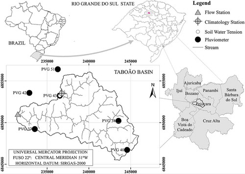
A rural river basin (Taboão basin) was taken for study with an area of 78 km², located in the northwest of the state of Rio Grande do Sul (Brazil), in the central part of the South American basalt flow (Fig. 2). This basin was considered representative of the Rio Grande do Sul basalt plateau region in terms of soil characteristics, relief and rainfall (Borges and Bordas 1988). Extensive agriculture is present in 88.5% of the basin area, and the practice of “non-till” cultivation predominates, soy beans and maize being the most common crops in summer, and wheat and oats in winter. With non-till cultivation, the soil is not turned over and the straw from the previous crop is left on the surface. The straw has a direct effect of preserving moisture in the surface layers of the soil by reducing solar radiation and temperature at the soil surface (Oliveira et al. 2010), besides acting as a mechanical barrier to surface runoff, thus increasing infiltration.

Figure 2. Localization of the study area, showing the position of the monitored points.

According to the Köppen classification system, the climate in the region is mild mesothermal of the temperate type, super humid and with no dry season (cfa) (Nimer 1989). The region has four well-defined climate seasons (spring: 22 September to 22 December, summer: 22 December to 22 March, autumn: 22 March to 22 June, and winter: 22 June to 22 September). The mean air temperature ranges from 14°C (May) to 24°C (January), reaching lower extreme temperatures of 0°C during winter and higher than 35°C in summer. The mean relative humidity of the air is 69%, with a minimum value of 65% (December) and maximum of 80% (July). Solar radiation is more intense during the period from October to March, attaining maximum values between November and January. Mean reference evapotranspiration is between 2.3 mm d⁻¹ (June) and 4.2 mm d⁻¹ (December), with an annual total around 1200 mm (IPAGRO 1989).

Rainfall is well distributed throughout the year, with no marked dry period. Mean annual precipitation was 1700 mm for the period 1961–2013 at the INMET station at Cruz Alta, located 18 km from the centre of the study basin. However, the region can be affected by extreme rainfalls associated with El Niño, and by extreme droughts associated with La Niña events.

The shape of the basin is elongated with the main axis toward the northwest. The relief varies from 340 to 490 m, with the highest altitudes found in the extreme east. The mean slope is 8%, although it varies between 10 and 20% in the valleys, and may reach up to 45% at some isolated points (Viero 2014). The basin’s soil classification was reported by Carvalho et al. (1990) and adapted to the new Brazilian soil classification system (EMBRAPA 2006). According to the soil classification system of the United States Department of Agriculture (USDA 1999), the predominant soil in the basin is Udox (94.9% in the basin area, which corresponds to the Brazilian classification of dystrophic-LVd red Latosol, dystroferric-LVdf red Latosol and eutroferric-NVef red Nitosol), characterized by great depth and amount of clay. There is also the presence of Fluvent (fluvic Neosol Tb eutrophic-RYbe) Udorthent (eutrophic Litholic Neosol-Rle) and Aqualf (haplic Gleysol-GX). The correspondence of the Brazilian soil classification was done according to Prado (2007).

3.2 Model input and output variables

With the resources available, 38 input variables in all were tested as inputs to the ANN models, the selected variables being those that physically influence soil moisture in space and time. Four of them describe basin topography (altitude, distance from the sampled point to the stretch closest to the river, difference of level between the sampled point and the stretch closest to the river, and slope); eight are related to soil physical properties (soil classification, soil density, resistance to soil penetration for the layers of 0–19 cm and 20–40 cm; % clay, silt and sand, and soil water tension); 10 describe climate (climate classification, maximum and minimum air temperature, grass temperature, global solar radiation, wind velocity, maximum and minimum relative humidity of air, atmospheric pressure and evapotranspiration); and 18 variables are related to rainfall (accumulated rainfall of 1, 2, 3, 4, 5, 6 and 12 preceding hours; accumulated rainfall of 1, 2, 3, 5, 10, 15, 20, 25 and 30 preceding days; exponentially weighted moving average of past hourly rainfall, and exponentially weighted moving average of past daily rainfall). For the soil classification, integer values from 1 to 5 were taken for the soil classes; integer values from 1 to 3 were taken to represent climate. Variables in the soil and topographical groups vary only spatially, and the climate variables vary only in time. The rainfall variables vary both spatially (because raingauges were different at different points) and temporally.

The accumulated rainfall data depend on other considerations: for example, when using accumulated rainfalls of 1 and 5 days as input variables, it was necessary to consider separately the rainfall accumulated over one day, and the rainfall that accumulated over the 5 days preceding the beginning of that day. This separation procedure was necessary because throughout this study it was observed that duplicated information adversely affected model performance.

The exponentially weighted moving average of past rainfalls (EWMA) was proposed by Moore (1980) to represent the soil moisture conditions in forecasting models based on the precipitation series. The procedure, in which the more recent rainfall values have a greater weight in the composition of EWMA, was used in this study both for hourly and for daily rainfalls, and had been used previously by Oliveira et al. (2013), with an excellent result for a sub-basin of the Ijuí river basin (Nash-Sutcliffe efficiency, NS = 0.95). The authors found that this moving average, when applied as an input variable, resulted in greater efficiency for the model when compared with the use of accumulated isolated rainfalls.

Both the hourly and daily exponentially weighted moving average of past rainfall were calculated based on:

(6)

where q_i = α(1 – α)ⁱ, P_t is the rainfall that occurred in time t; and α is a weighting coefficient.

The coefficient α is related, for a unit time interval, to the half-life h by:

(7)

Choosing L to have a half-life of h days means that the contribution of rainfall h days ago to the current value of EWMA is reduced by one-half.

Several half-life alternatives were tested, for both the hourly and the daily rainfall, and those that presented the best correlation with soil moisture were selected.

After selection of the most representative half-life, slightly higher or slightly lower values were also tested in the ANN models, always choosing the one that would give the best results when applying the model. A half-life of 1.2 h was used for the hourly exponentially weighted moving average, while for the daily exponentially weighted moving average, 0.5 d was used.

The models’ output variable, representing moisture at points in the basin, was compared with gravimetric moisture determined from samples collected in the field. To determine the physical properties of soil and gravimetric moisture, 26 collection points were selected in the basin, distributed over the different types of soil and altitudes.

3.3 Artificial neural networks

The three-layer MLP network was used in this study with the unipolar sigmoid activation function adopted for all neurons; training was performed by the back-propagation algorithm, applying cross-validation. The number of neurons in the inner layer was initially adopted by the rule 2n+1, following the theorem given by Hecht-Nielsen (1987), where n is the number of input variables. After preliminary tests, together with experiments comparing performance when alternatives close to this number were used, the number of 25 neurons was chosen for all models. The ANN training was performed with the authors’ personalized software developed for use of the back-propagation algorithm, and programmed in the software environment of MATLAB® 7.12.0 R2010a. The method of Vogl et al. (1988) was used for the convergence acceleration.

Several iterations were performed for training, each of them with random initializations of the synaptic weights, adopting the resulting weights of the iteration with the best final performance, so as to minimize the influence of the random initialization over the results. After preliminary tests, it was concluded that no more than 10 iterations would be needed, but 16 were used for safety.

The set formed by the network specification (activation function adopted and number of neurons in the inner layers), by the synaptic weights and also by the parameters for staggering the input and output variables (considering the limitations of the activation function domain) define the complete model consisting of the neural network.

Twenty-five soil samples were collected, to estimate soil moisture at each of the 26 points (Fig. 3) in the period from 15 January to 10 August 2013, comprising the summer (the dry season with the largest evapotranspiration), autumn and winter (the wet season). Each sample was collected over four consecutive days; measurements from the first and third days (at each of the 26 points) were used for the training series, those from the second day were used for the validation, and those from the fourth day for verification. This selection procedure for the training, validation and verification series was used so that the training series were representative, with soil moisture values corresponding to those of summer and winter. Thus, the separation of the samples to apply the cross-validation method covered 50% of the data for training, 25% for validation and 25% for verification, but additional care was taken to be sure to have included in the training series the records with extreme values of input and output variables, so that the resulting domain for the variables in the training series would be comprehensive regarding the domains observed in the other series.

After training, the complete model was applied to the verification series to evaluate the quality of the model by comparing these results with the values observed, by visual inspection and by calculating performance statistics. The performance statistics used were functions of the errors: namely, the maximum absolute error (Ea(max)), the 95% quantile of the error distribution (Ea(95)), the mean absolute error (Ea(mean)), the square root of the mean quadratic error (RMSE) and the Nash-Sutcliffe statistic (NS), also calculated based on the errors. The respective equations for Ea(mean), RMSE and NS are as follows:

(8)

(9)

(10)

where y_j is the jth observation of the variable evaluated; is the jth simulation of the variable evaluated; is the mean of the set of values observed, and N is the total number of measurements.

More than 200 models based on ANNs were tested to estimate SWC. The same network configuration was considered for all tests performed, i.e. the same number of neurons (25) in the inner layers, together with the same number of iterations (16). An attempt was made to carry out as many cycles as needed to reach the optimum training point – the point at which overfitting began. Each application was verified by looking at the simultaneous time variation graph of the sums of quadratic deviations of the training and validation samples, the result varying between 30 000 and 300 000 cycles. The same training, validation and verification series were used in all situations tested, but with different combinations of input variables in each of the models analysed.

Table 1 shows the results of physical analysis of watershed soil and topography that were used as input variables in the ANN models tested, considering the 26 points at which soil samples were collected to determine gravimetric moisture, on the dates of the 24 field campaigns. These variables are characteristics of each point, and do not vary over time. The inputs are related to the physical properties of soil (soil classification, soil density, resistance to penetration in soil for 0–19 cm and 20–40 cm layers, and percentages of sand, silt and clay), to the topographic characteristics (altitude, slope and distance from that point to the closest river reach, difference in level from that point to the closest river reach), besides the rainfall records used to calculate accumulated and exponentially weighted moving averages.

Table 1. Soil physical properties, topographic basin properties and raingauges used to give accumulated rainfall, considering the 26 sample points and the dates of the 24 field campaigns.

Point	Altitude (m)	Soil classification	Raingauge	Distance: point closest to river (m)	Slope (°)	Density (g cm^−3)	Resistance to soil penetration		Sand (%)	Silt (%)	Clay (%)
							0–19 cm (kPa)	20–40 cm (kPa)
P01	351	NVef (3)	37/42	43	2.62	1.40	1371.70	2116.95	16.52	38.44	45.04
P02	410	LVd2 (2)	37	566	0.00	1.64	2384.90	2499.95	13.77	35.43	50.80
P03	382	LVdf2 (5)	37	181	8.33	1.53	1964.90	2858.29	15.33	20.88	63.79
P04	419	LVdf2 (5)	42	333	5.31	1.64	1264.90	2083.33	19.99	32.76	47.25
P05	429	LVdf1(4)	42	509	5.31	1.58	1267.00	1530.29	15.87	35.82	48.31
P06	396	NVef (3)	43	78	8.41	1.46	1378.55	1855.81	11.88	33.67	54.45
P07	378	NVef (3)	43	42	5.56	1.54	1197.65	1712.48	18.50	38.62	42.88
P08	397	LVd1(1)	43	214	0.00	1.60	1550.70	1841.71	18.16	37.56	44.28
P09	435	LVd1 (1)	43	335	0.00	1.58	1384.40	1926.81	20.74	27.84	51.42
P10	433	LVdf2 (5)	43	220	3.53	1.69	1302.90	2486.00	16.70	19.79	63.51
P11	389	NVef (3)	43	236	0.65	1.56	1712.65	2635.14	17.00	25.64	57.36
P12	455	LVdf1(4)	51	170	2.64	1.52	1325.15	2460.14	15.49	19.84	64.67
P13	448	LVdf2 (5)	51/43	174	4.61	1.56	1187.20	2637.67	14.66	29.21	56.13
P14	427	NVef (3)	43/51	187	7.64	1.63	1544.15	1711.81	16.99	35.55	47.46
P15	417	NVef (3)	43/51	18	7.39	1.51	1287.70	2976.52	23.66	29.41	46.93
P16	411	LVd1 (1)	43/34	286	2.53	1.45	1869.10	2485.95	27.64	27.32	45.04
P17	415	LVdf2 (5)	34	252	2.91	1.47	1067.75	1786.52	18.52	26.23	55.25
P18	402	NVef (3)	34	21	4.66	1.59	1167.85	2606.67	30.81	21.00	48.19
P19	452	LVd2 (2)	34	189	3.85	1.60	2237.90	1945.19	32.98	27.54	39.48
P20	457	LVd2 (2)	40	429	2.17	1.49	1279.95	1868.90	24.78	24.51	50.71
P21	477	LVd2 (2)	34	484	0.00	1.55	1007.15	2301.00	18.78	26.95	54.27
P22	446	LVd2 (2)	34	99	5.26	1.69	1984.95	2813.62	31.84	17.08	51.08
P23	474	LVd1 (1)	34/40	265	0.00	1.61	1330.80	1801.29	52.02	23.69	24.29
P24	483	LVd1 (1)	34	111	4.40	1.68	1339.65	2077.38	50.32	14.63	35.05
P25	470	LVd1 (1)	40	329	2.15	1.60	1333.35	2366.19	38.00	21.50	40.50
P26	483	LVd1 (1)	40	191	0.00	1.73	2732.45	3009.57	38.00	21.50	40.50

3.4 Obtaining the data

3.4.1 Physical properties of soil

All the 650 samples collected were on Udox soil, at 26 points, corresponding to five soils according to the Brazilian classification; counting the subgroups, there were nine soil types altogether (Fig. 3). These soils constitute 89.8% of all soils in the basin.

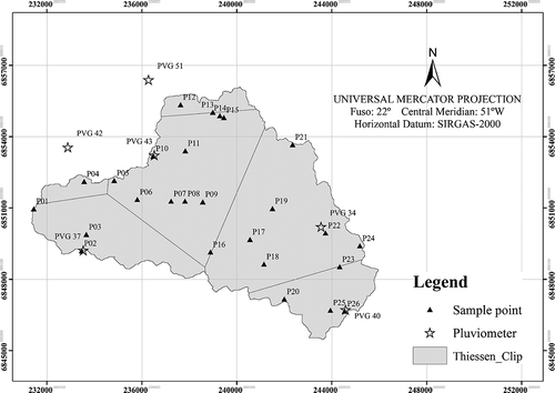
Figure 3. Raingauge distribution at Taboão basin and the influence of each gauge at 26 soil sampled points, using the Thiessen method (Thiessen 1911).

To determine gravimetric moisture, mixed samples of soil were collected (soil mass: 400–600 g) at the soil surface (between 5 and 15 cm depth) in triplicate. Plant and crop residues on the surface were removed. Four collections were performed at 24-h intervals in every month (15, 16, 17 and 18 January; 19, 20, 21 and 22 February; 20, 21, 22 and 23 March; 1, 2, 3 and 4 May; at 05:00, 06:00, 17:00 and 18:00 h, 7 and 8 June; 7, 8, 9 and 10 August 2013), a total of 25 collections on 24 dates (06 June: collections performed at two points in time – morning and afternoon) between January and August 2013. Gravimetric moisture was calculated as the ratio of water mass contained in the sample (difference between the wet and dry weights) to mass of dry soil. The median value of the triplicate measurements was used for network training and validation, thus avoiding possible errors generated by the existence of extreme values.

Soil density was defined as the ratio of dry soil mass to sample volume, and was calculated from un-mixed samples (between 5 and 15cm depth) obtained using volumetric rings (approximately 64 cm³), also in triplicate, at each of the 26 points monitored; the density at each point was obtained by the median of the triplicates. These measurements were made on 8 and 9 August 2013.

Resistance to soil penetration was determined for layers of 0–19 cm and 20–40 cm. These measurements were performed using the PenetroLOG (Electronic Soil Compaction Meter, Falker S.A.) equipment. This gives precise measurements in soil layers up to 60 cm deep, enabling the identification of the physical conditions of soil (pressure corresponding to soil compaction in the layer) at several depths, at the chosen points. The measurements were obtained between 28 April and 3 May 2014.

Soil grain size at each of the points was obtained in the laboratory by sieving and pipetting. Mixed samples of soil were collected from 5–15cm depth, in triplicate. The samples were collected over the same period in which the resistance to soil penetration was measured. The collected material first underwent the process of burning the organic matter with hydrogen peroxide and through physical and chemical disaggregation, after which it was sieved (up to 0.0063 mm) and pipetted (<0.0063 mm).

Soil water tension was monitored daily by an observer throughout the period of this study, using a tensiometer installed at a depth of 10 cm from the soil surface. The data used concern the 24 days when soil samples were collected.

3.4.2 Climate information

Climate records (maximum and minimum daily air temperature, maximum and minimum relative air humidity, daily mean atmospheric pressure, global solar radiation and daily mean wind velocity) were supplied by the Instituto Nacional de Meteorologia (INMET), and the data for the historical series were from the climatology station installed at the city of Cruz Alta (Rio Grande do Sul, Brazil), 18 km from the basin (UTM coordinates: 238 553 m E and 6 833 021 m S, Zone 22J). The data used were those from the 24 days on which soil samples were collected.

Reference evapotranspiration was calculated using the Sistema para Manejo da Agricultura Irrigada – SMAI (System for the Management of Irrigated Agriculture) software (Mariano et al. 2011) using the Penman-Monteith equation (Allen et al. 1998), with the climate variables recorded at the INMET climatology station of Cruz Alta. In addition, data on the temperature on grass (monitored in the basin) were used, and an input variable termed “climate”, according to the seasons of the year (1: summer, 2: autumn, 3: winter).

3.4.3 Rainfall information

Rainfall was monitored by six raingauges (of the tipping bucket type) in the watershed, which recorded rainfall every 10 min. The Thiessen polygon method (Thiessen 1911) was used to delimit the area of influence of each gauge at each of the soil collection points, and also to delimit which gauge would be used for each point (Fig. 3). In situations where the point was located between two polygons, the observations at the two gauges corresponding to the areas delimited by the adjacent polygons were used. At six of the collection points considered (P01, P13, P14, P15, P16 and P23) two gauges were used, because those points were located close to the two polygons.

The rainfall series used were different for each soil collection point because the reference for the respective time positions was the time of day at which collection was performed at each point, and, since the basin area is 78 km², the soil was collected at different times of day, although always on the same day, because of the time taken for travel between points.

3.4.4 Topographical information on the basin

The input variables related to topography (altitude, slope, distance from the point of collection to the closest river reach and difference in level from that point to the closest river reach) were extracted from the Numerical Terrain Model (NTM) with a 90-m resolution, using the ArcToolbox tool of ARCGIS (ESRI®). The collection points lie at altitudes ranging from 340 to 473 m, with a slope varying from 0.0 to 14.8%, and the distance from the point to the closest river reach varies from 18 to 566 m.

3.5 Preliminary analysis

Descriptive statistics were calculated (minimum, maximum, mean, median and standard deviation) of the 38 input variables, as well as the Pearson correlation coefficient between each of them and the soil moisture, in order to know its amplitude of variation and to get a first approximation of its importance to the modelling of the water content. Although the ANNs can approximate complex nonlinear phenomena, a high absolute value of the linear correlation is an indicator that the variable is promising as model input for the estimation of soil moisture.

4 Results and discussion

4.1 Analysis of descriptive statistics on input variables and correlation with soil water content

Soil density varied from 1.40 to 1.73 g cm⁻³. The resistance to soil penetration ranged between 1007.15 and 2732.45 kPa for the 0–19-cm layer and between 1530.29 and 3009.57 kPa for the 20–40-cm layer. The percentage of sand varied from 11.88 to 52.02%, while that of silt varied from 14.63 to 38.62%, and of clay, from 24.29 to 64.67%.

The maximum value recorded for soil water tension was equal to 0.83 bar, and the minimum was 0.06 bar, with a mean of 0.26 ± 0.23 bar, and median of 0.14 bar.

Table 2 shows descriptive statistics of all variables. Except for soil classification and the “climate” variable, all variables are quantitative.

Table 2. Descriptive statistics of variables used as input and output to the ANN models, considering 24 dates from 10 January to 15 August 2013. SD: standard deviation.

	Parameter	Group	Minimum	Maximum	Mean	Median	SD
1	Altitude (m)		351.00	483.00	428.81	428,00	34.71
2	^1Distance (m)	Topographic	19.00	594.00	298.46	274.50	195.62
3	^2Level (m)		0.00	36.25	10.48	9.92	8.73
4	Slope (%)		0.00	8.41	3.46	3.22	2.67
3	^3Soil classification (-)		1.00	5.00	2.73	3.00	1.43
4	Soil density (g cm^−3)		1.40	1.73	1.57	1.58	0.08
5	^4Res. pen. 0–19 cm		1007.15	2732.45	1518.28	1336.50	420.78
6	^4Res. pen. 20–40 cm		1530.29	3009.57	2245.97	2208.98	425.38
7	% Clay	Soil	24.29	64.67	48.79	48.25	8.88
8	% Silt		14.63	38.62	27.40	27.14	6.77
9	% Sand		11.88	52.02	23.81	18.65	10.71
10	Soil water tension (bar)		0.06	0.83	0.26	0.14	0.22
11	^5Climate (-)		–	–	–	–	–
12	^6Max. air temp. (°C)		6.70	30.90	22.99	23.60	4.89
13	^6Min. air temp. (°C)		4.90	28.80	16.31	15.40	7.18
14	^6Grass temp. (°C)		12.00	31.60	18.51	18.70	4.17
15	^6Global solar radiation (kJ m^−2 d^−1)		974.47	4531.18	2125.79	1755.51	910.83
16	^6Mean wind velocity (m s^−1)	Climate	0.10	6.50	2.58	2.65	1.51
17	^6Max. relative humidity of air (%)		78.20	97.00	91.44	94.00	5.62
18	^6Min. relative humidity of air (%)		35.00	92.00	64.92	67.00	19.17
19	^6Mean atmos. pressure (hPa)		958.15	972.79	965.75	965.93	3.06
20	^6Ref. evapotranspiration (mm)		0.90	8.00	3.71	3.40	1.80
21	^7Acc. rainfall of 1 h (mm)		0.00	2.20	0.07	0.00	0.32
22	^7Acc. rainfall of 2 h (mm)		0.00	4.00	0.13	0.00	0.60
23	^7Acc. rainfall of 3 h (mm)		0.00	6.40	0.19	0.00	0.85
24	^7Acc. rainfall of 4 h (mm)		0.00	7.90	0.24	0.00	1.02
25	^7Acc. rainfall of 5 h (mm)		0.00	9.15	0.29	0.00	1.12
26	^7Acc. rainfall of 6 h (mm)		0.00	9.35	0.32	0.00	1.18
27	^7Acc. rainfall of 12 h (mm)		0.00	36.01	1.34	0.00	4.61
28	^8Acc. rainfall of 1 d (mm)		0.00	56.00	2.73	0.20	9.17
29	^8Acc. rainfall of 2 d (mm)	Rainfall	0.00	56.20	6.34	0.40	13.63
30	^8Acc. rainfall of 3 d (mm)		0.00	56.40	10.71	1.60	16.50
31	^8Acc. rainfall of 5 d (mm)		0.00	56.40	19.26	18.30	17.35
32	^8Acc. rainfall of 10 d (mm)		0.00	110.00	33.37	24.60	24.30
33	^8Acc. rainfall of 15 d (mm)		0.00	163.83	51.87	32.80	44.03
34	^8Acc. rainfall of 20 d (mm)		1.80	186.98	70.51	54.80	47.22
35	^8Acc. rainfall of 25 d (mm)		1.80	201.80	88.27	80.50	44.57
36	^8Acc. rainfall of 30 d (mm)		2.00	231.83	113.57	90.00	47.78
37	^9EWMA of past hourly rainfall (mm)		0	1.878	0.092	0	0.291
38	^9EWMA of past daily rainfall (mm)		0	42	2.929	0.45	7.066
–	Soil water content (%)	Output	13.93	36.75	24.88	25.47	3.83

¹distance from the collection point to the stretch closest to the river; ²difference of level between the point and the stretch closest to the river; ³soil classification (1: LVd red Latosol dystroferric1, 2: LVd red Latosol dystroferric2, 3: NVef red Nitosol, 4: LVdf red Latosol eutroferric1, 5: LVdf red Latosol eutroferric2); ⁴resistance to soil penetration for the 0–19 cm and 20–40 cm layers; ⁵climate (1: summer, 2: autumn and spring, 3: winter); ⁶data from the climatology station in Pejuçara at the centre of the watershed; ⁷accumulated rainfall of preceding hours; ⁸accumulated rainfall of preceding days; ⁹EWMA: exponentially weighted moving average.

Table 3 gives the correlations between each of the 38 input variables and SWC. Positive correlations indicate that soil moisture increases as the variable increases in value, and vice versa.

Table 3. Linear correlation between input variables and the soil water content.

Variable	Correlation, r	Variable	Correlation, r	Variable	Correlation, r
Altitude (m)	0.45	Minimum air temperature (°C)	–0.3963	Accumulated rainfall of 12 h (mm)	0.2076
Distance (m)	–0.2702	Grass temperature (°C)	–0.2983	Accumulated rainfall of 1 d (mm)	0.1470
Level (m)	0.0672	Global solar radiation (kJ m^−2 d^−1)	–0.3822	Accumulated rainfall of 2 d (mm)	0.1382
Slope (%)	0.3016	Mean wind velocity (m s^−1)	0.0533	Accumulated rainfall of 3 d (mm)	0.0968
Soil classification (-)	0.4074	Maximum relative humidity of air (%)	0.4689	Accumulated rainfall of 5 d (mm)	0.1428
Soil density (g cm^−3)	–0.3626	Minimum relative humidity of air (%)	–0.1888	Accumulated rainfall of 10 d (mm)	0.0722
Res. pen. 0–19 cm	–0.2401	Mean atmospheric pressure (hPa)	–0.0337	Accumulated rainfall of 15 d (mm)	–0.0830
Res. pen. 20–40 cm	0.0018	Reference evapotranspiration (mm)	–0.3909	Accumulated rainfall of 20 d (mm)	–0.1354
% Clay	0.3600	Accumulated rainfall of 1 h (mm)	0.2780	Accumulated rainfall of 25 d (mm)	–0.1599
% Silt	0.3346	Accumulated rainfall of 2 h (mm)	0.2707	Accumulated rainfall of 30 d (mm)	–0.2390
% Sand	–0.5078	Accumulated rainfall of 3 h (mm)	0.2691	EWMA of past hourly rainfall (mm)	0.3082
Soil water tension (bar)	–0.3321	Accumulated rainfall of 4 h (mm)	0.2556	EWMA of past daily rainfall (mm)	0.1542
Climate (-)	0.3559	Accumulated rainfall of 5 h (mm)	0.2471
Maximum air temperature (°C)	–0.1659	Accumulated rainfall of 6 h (mm)	0.2619

Table 4. Statistical performance of selected models.

Model	M02	M03	M05	M08	M69	M70	M71	M78
Number of cycles (mil.)	300	100	30	30	100	30	30	30
Number of nodes	9	25	25	25	25	25	25	25
J^1	44 516	30 877	478	4542	4534	3061	7321	17 135
Input variables^2	1 to 4	5 to 12	13 to 22	23 to 38	1, 2, 4 to 8, 35, 37, 39, 40	1 to 38	1, 2, 4, 5, 7 to 12, 35, 37, 39, 40	1, 3, 4, 35, 37, 39, 40
Training
Ea(95)	5.85	4.70	6.71	6.18	4.46	4.16	4.11	4.64
Ea(max)	10.63	8.99	9.81	9.41	7.99	8.10	8.08	8.75
Ea(mean)	2.28	1.69	2.56	2.44	1.56	1.53	1.51	1.76
RMSE	2.94	2.33	3.27	3.11	2.08	2.00	2.05	2.32
NS	0.41	0.63	0.27	0.34	0.70	0.72	0.71	0.63
Verification
Ea(95)	6.22	6.12	6.32	6.82	3.71	5.52	3.63	4.59
Ea(max)	8.91	7.83	9.61	9.79	7.54	9.30	8.61	6.43
Ea(mean)	2.62	2.34	2.85	2.81	1.52	2.09	1.54	1.96
RMSE	3.27	2.96	3.54	3.48	2.01	2.65	2.02	2.47
NS	0.39	0.50	0.28	0.32	0.77	0.61	0.77	0.65

¹J: number of cycles needed for the best model result, without overtraining occurring.

²Input variables: 1: altitude; 2: distance from the collection point to the stretch closest to the river; 3: difference of level between the point and the stretch closest to the river and slope; 4: slope. 5: soil tension at a point; 6: soil classification (1: LVd1; 2: LVd2; 3: NVef; 4: LVdf1; 5: LVdf2); 7: density; 8: resistance to soil penetration for the 0–19 cm layer; 9: resistance to soil penetration for the 20–40 cm layer; 10: sand; 11: silt; 12: clay; 13: temperature on the grass; 14: climatology station; 15: maximum air temperature; 16: minimum air temperature; 17:maximum relative humidity of air; 18: minimum relative humidity of air; 19: mean atmospheric pressure; 20: global solar radiation; 21: mean wind velocity; 22: calculated reference evapotranspiration; 23: accumulated rainfall preceding 1 h; 24: accumulated rainfall preceding 2 h; 25: accumulated rainfall preceding 3 h; 26: accumulated rainfall preceding 4 h; 27: accumulated rainfall preceding 5 h; 28: accumulated rainfall preceding 6 h; 29: accumulated rainfall preceding 12 h; 30: accumulated rainfall preceding 1 d; 31: accumulated rainfall preceding 2 d; 32: accumulated rainfall preceding 3 d; 33: accumulated rainfall preceding 5 d; 34: accumulated rainfall preceding 10 d; 35: accumulated rainfall preceding 15 d; 36: accumulated rainfall preceding 20 d; 37: accumulated rainfall preceding 25 d; 38: accumulated rainfall preceding 30 d; 39: exponentially weighted moving average of past hourly rainfall; 40: exponentially weighted moving average of past daily rainfall.

Fourteen variables had correlations greater than 0.3 in absolute value. The largest correlations of these were for sand percentage, maximum relative humidity of air, and altitude (–0.51, 0.47 and 0.45, respectively). This is understandable because sandy soils have higher water retention due to their macroporosity, while the higher the air humidity, the higher the SWC, due to the lower evapotranspiration and by the eventual occurrence of rainfall. Altitude is correlated with soil moisture (Famiglietti et al. 1998, Zhu and Lin 2011), since the points located on higher ground are farther from the groundwater table or the saturated zone.

Fifteen variables gave correlations less than 0.2 in absolute value, of which eight are for accumulated rainfalls from 2 to 25 days. This indicates that more recent rains (hourly accumulated rainfall and exponentially weighted moving average of past rainfalls) have more influence on SWC than accumulated rainfall from several previous days. In this region, the high potential evapotranspiration in summer (6.9 mm d ⁻¹, Beltrame et al. 1994) takes several days to reduce the soil water storage substantially, while in winter, with potential evapotranspiration around 0.4 mm d⁻¹ (Beltrame et al. 1994), it takes longer. Therefore, the accumulated rain some hours before collecting the soil samples is important when estimating SWC both in summer and in winter, whereas the daily accumulated rainfall is important only in winter, resulting in larger hourly accumulated rain correlations.

4.2 Analysis of descriptive statistics on soil water content

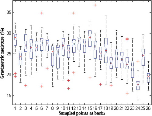
Measured gravimetric moisture varied between 13.93 and 36.75%, with a mean of 24.88 ± 3.25% and median of 26.10%. Figure 4 shows a box plot graph of gravimetric moisture distribution in the 25 collections performed for each of the 26 sites sampled.

In general, the variation of the median, and of the maxima, minima and standard deviation of gravimetric moisture too, was lower during winter, attaining greater variations in summer, when temperatures are higher. Indeed, the lowest moisture was found during summer on 19 February 2013, for the point PN4 (24th point in Fig. 4), which is located at an altitude of 483 m. In contrast, the highest gravimetric moisture was found during winter on 8 October 2013, for point PN9 (16th point in Fig. 4), located at an altitude of 411 m. Both points have Udox soil (Dystrophic Red Latosol – subclass LVd1). In fact, the results obtained are consistent, since it is expected that in summer the SWC will be less, because temperatures are higher during this period, causing a greater evaporative demand for water in soil, and greater evapotranspiration (in the present case during soy bean cultivation in the basin studied). In addition, point PN4 is at a higher altitude and, as pointed out in previous studies (Famiglietti et al. 1998, Zhu and Lin 2011), the SWC tends to be lower at higher altitudes than at lower ones, which receive the waters drained from a greater number of contributing zones. The highest moisture was found during the winter and at the lowest point in the relief, confirming the influence of climate and relief on soil water storage.

Figure 4. Box plot of gravimetric soil moisture for each sampled site.

These characteristics show that there is a spatial and temporal variation in SWC in the basin over the study period, indicating that both the physical characteristics of the basin (physical properties of soil and topographical properties of the basin), and the climate characteristics influence SWC.

4.3 Estimation of soil water content using models based on ANNs

Table 4 gives the performance statistics for the eight main ANN models analysed. These were obtained during network training and verification. The models were selected based on the following factors: best performance during verification; good model performance during verification and ease of obtaining the input variables (climatological, topographical and soil classification data in the public domain) and good model performance in verification; and need for few input variables or easily obtained input variables. Also presented are the models that use only the variables of each of the groups (physical properties of soil, basin topography, rainfall or climatological variables without rainfall data), and a model that utilizes all the available input variables.

In the training process, the NS statistic given by the eight models varied from 0.27 to 0.72; during verification, it varied from 0.28 to 0.77. The two best models observed (models considered most appropriate to the situation analysed in the study) were M69 and M71, which use information related to basin topography and the physical properties of soil and rain, with 11 and 13 variables, respectively.

Model M69 used 11 input variables: altitude, distance from the point to the reach closest to the river, slope, soil water tension, soil classification, soil density, resistance penetration in soil to the layer from 0–19 cm, the 15 and 25 day rains, and the hourly (EWMA hourly) and daily weighted (EWMA daily) rains. This network gave NS statistics of 0.70 and 0.77, Ea(95) of 4.46 and 3.71%, Ea(max) of 7.99 and 7.54%, Ea(mean) of 1.56 and 1.52%, and RMSE equal to 2.08 and 2.01% for training and verification, respectively. In contrast, model M71 has 14 input variables and is different from the previous one because it uses as input the percentage of sand, silt and clay, instead of the soil classification variable, and resistance penetration in soil to the 20–40 cm layer. This network gave NS statistics of 0.71 and 0.77, Ea(95) of 4.11 and 3.63%, Ea(max) of 8.08 and 8.61%, Ea(mean) of 1.51 and 1.54%, and RMSE of 2.05 and 2.02% for training and verification, respectively.

Of these 14 input variables, nine had absolute correlations higher than 0.3 (% sand, altitude, soil classification, soil density, % clay, % silt, soil water tension, hourly EWMA and slope). The other five variables, although having smaller correlations, were selected for models because they were able to take advantage of the nonlinear relationships between these variables and the soil moisture.

Three of these 14 variables are topographic variables. The altitude and the slope have their importance recognized as variables that influence soil moisture. The higher the values of these variables, the lower the SWC, since the former represents the distance from the water table and the largest slopes favour the runoff. However, the work reported here included a new variable, represented by the distance from the sample point to the river, since points near the river, even in high terrain sites, are more prone to higher SWC than the points at the same altitude but farther from the river, due to the greater proximity to the water table.

As for the soil variables, high soil density values mean that there is less space between the pores, so that SWC retained in the porous space is smaller. Melo and Pedrollo (2015) analysed data from 228 soils around the world, contained in UNSODA database, using ANN, and found that the soil density was the soil property that most influenced the performance of the tested models for the water retention curve, improving the model efficiency by 46%. The same argument applies to the resistance to soil penetration: greater resistance to penetration results in greater density, which discourages water retention in the soil. The soil classification is a variable that encompasses these two characteristics, being related to the soil porosity, with the texture and structure of the soil, among other characteristics, such as organic content. So this is an important variable for estimating SWC. Soil texture describes the relative proportions of granulometric fractions observed in the mineral fraction of the soil. The higher the proportion of smaller size fractions, the higher the specific area per unit mass, the higher the possibility of cation exchange, the higher the soil capacity to store water and to bind the organic fraction, thus improving soil stability (Mello 2006), which contributes to the higher retention of water in the soil. The soil structure, in turn, refers to the grouping and arrangement of primary particles (clay, sand, organic matter, calcium, magnesium and free iron oxide) in the form of aggregates (WMO 2003, de Carvalho 2008). The water storage in soil at the wettest band, near saturation, in the soil water retention curve is strongly governed by the soil structure and not its texture, since the texture, in turn, is influenced more strongly by the water flow in the micro- and mesopores at the most negative potentials (Mermoud and Xu 2006). In addition, the organic matter content, for example, is considered important in pedotransfer functions to estimate the SWC due to an increase in water retention capacity (Ahuja et al. 1985, Brady 1989, Rawls et al. 2003). This variable can be considered as similar to the “soil classification” variable, although not in detailed form, because this depends on the land use strategies used by different farmers.

Another important variable to represent SWC is the water tension in the soil, since the curve that relates it to the water tension in the soil is well known (Arya et al. 1999, Schaap et al. 2004, Walczac et al. 2006): the lower the tension, the higher the SWC. This variable was important as input for the two models M69 and M71, and has been shown to represent the spatial variability of the SWC (in the 26 well-distributed points in the bowl), although the value of the tension used as input corresponded to just one point across the basin of 78.4 km².

Regarding the time variation in SWC, represented by the accumulated rainfall, it was expected that previous accumulated rainfall was the most important variable for estimating the SWC. However, the number of hours or days prior to the accumulation of rain, which influences the SWC, was unknown. For the M69 and M71 models, each with 18 accumulated rainfall variables tested, four rainfall input variables were the most important: namely, the accumulated rainfalls of 15 and 25 days, and the exponentially weighted moving average of past hourly and daily rainfalls, with adjusted half-life of 1.2 hours and 0.5 days, respectively.

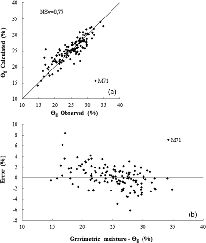
Figures 5 and 6 show the relation between observed and calculated gravimetric moisture, compared to the best-fitting line, as well as the error (discrepancy) between the values calculated and observed considering the process of verifying the models with the best performance (M69 and M71).

These two models (M69 and M71) behaved very similarly, giving performance statistics in close agreement. However, M71 has a slightly better error distribution around the axis zero, indicating that the discrepancies in estimating gravimetric moisture are slightly lower in this model. The adjustment between the values observed and calculated is very good for both models, with a few values very close to the best-fit line (Figs 5(a) and 6(a)), and although some extremes are not well represented, the errors are relatively well distributed (Figs 5(b) and 6(b)), and the number of underestimated and overestimated values is very close (66 and 68, respectively, for the two models). Both models can very satisfactorily follow the variation of gravimetric moisture behaviour over time (Figs 5(a) and 6(a)).

Figure 5. Observed and calculated gravimetric moisture in relation to ideal adjustment: (a) 1:1 line; and (b) error between observed and calculated gravimetric moisture for the best performing model, M69.

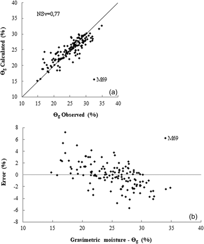
Figure 6. Observed and calculated gravimetric moisture in relation to ideal adjustment: (a) 1:1 line; and (b) error between observed and calculated gravimetric moisture for the best performing model, M71.

Collections and field measurements of variables related to physical properties of soil (soil density and resistance to penetration in soil, besides grain size for model M71) specific for each point of interest were required by models M69 and M71. However, it is important to emphasize that the determination of the percentages of sand, silt and clay for each point of interest (input variables required in model M71) requires more time and financial resources for collection and processing than soil classification (the input variable needed for model M69). The latter can be obtained directly from a previously constructed map of types of soil, which simplifies the process of acquiring the information for a new point of interest.

In a comparison by groups of input variables, the model that uses only the physical properties of soil (M03) performed better (NS of 0.63 and 0.50 for training and verification, respectively) than the other three models that used information only on properties related to the basin topography (M02, NS = 0.41 for training, and NS = 0.39 for verification), rainfall (M08, NS = 0.34 for training and NS = 0.32 for verification) and climate without rainfall (M05, NS = 0.27 and 0.28 for training and verification, respectively). In general, none of the models with inputs by group fitted the extremes of gravimetric moisture well, the values greater than 25% being underestimated by the models and the lower ones overestimated. This indicates that the physical properties of soil are most important for the estimation of SWC, though when rainfall and topography variables are added, such as in the M69 and M71 models, the results were significantly improved. Of the eight input variables of the model M03, six were among the top 12 absolute linear correlations, considering the 38 variables.

Model M05, which used only climate information, showed the worst agreement between the fitted values and the observed data, and did not manage to represent the behaviour of gravimetric moisture over time, underestimating or overestimating the values observed considerably, exerting little influence over the estimation of SWC. This characteristic may be related to the presence of plant cover and straw on the soil surface, which keeps the temperature of the surface stable, preventing the direct action of sunlight and limiting the evaporation processes, and consequently maintaining the SWC on the surface of the soil. Thus, it can be inferred that the climate variables (without considering rainfall) have little influence on the estimation of water contents stored in the soil. Elshorbagy and Parasuraman (2008) also observed that the climate information (daily mean values of precipitation, air temperature, soil temperature in the peat and in the soil layers, and solar radiation) did not have much influence on the estimation of soil moisture at different depths and with different plant cover. The network developed by the authors presented an adjustment between calculated and observed moisture, very similar to the one found in the present research.

This analysis by groups of input variables shows that, for the situation analysed in this basin, the use of antecedent rainfall information alone, or even its joint use with climate data, is not enough to estimate SWC adequately, considering the spatial and temporal variability. Thus it is necessary to make joint use of data related to the physical properties of the soil and to basin topography in order to obtain satisfactory results.

Model M70, which contains 38 input variables (all the variables minus the two weighted rainfalls) and 25 neurons at the intermediate layer, presented good performance in training (NS = 0.72), but a relatively lower performance during the verification of the network capacity to generalize (NS = 0.61). This model may be using duplicated information (due to the presence of similar variables) and confounding the ANNs, even though it performed satisfactorily in training and verification. Often this characteristic tends to generate a reduction in network performance and, therefore, the removal of some variables may improve model efficiency (Oliveira et al. 2011).

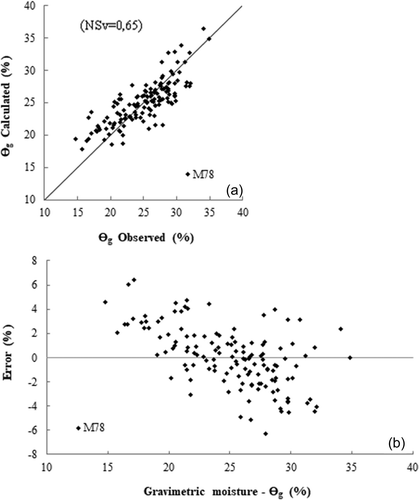
It should also be recalled that the requirement for a large number of input variables (such as for M70) may be a limiting factor when applying these models to estimate SWC, since the acquisition of input information for them requires a greater expenditure of funds and time. Thus, the use of more simplified models, with the input of more easily acquired and less expensive variables, may be useful in some situations in which data are restricted. In particular, the model M78, which needs little or no field data, with data on relief taken from maps and from rainfall records, could be used in situations in which the precision required to estimate SWC is not extremely strict, or for cases in which not many data are monitored at the site of interest, or even when there are not many resources available to obtain this information. It is clear that the performance of the simplified models is reduced when compared to the best models (M69 and M71), but they still performed fairly well.

Figure 7 shows the relationship between the calculated and the observed gravimetric moisture, in analogy with the line of best fit, and the relationship between the error found (discrepancy among the calculated and observed values) for model M78, whose explanatory variables are only those related to basin topography (altitude, slope and height difference) and to rainfall (15- and 25-day accumulated rainfall and hourly and daily exponentially weighted average rainfall).

Similarly to the case of models in which inputs are made by group (M02, M03 and M08), model M78 tends to underestimate the gravimetric moisture values higher than 25%, and to overestimate those lower than this percentage (Fig. 7(a) and (b)). Generally, this model can provide a good representation of the variation of gravimetric moisture, although it does not fit the extremes well (Fig. 7(a)).

Figure 7. Observed and calculated gravimetric moisture in relation to ideal adjustment: (a) 1:1 line; and (b) error between observed and calculated gravimetric moisture for the best performing model, M78, with topographic variables and exponentially weighted moving average of past hourly and daily rainfall.

5 Conclusions

This study investigated the possibility of estimating spatial and temporal variations of soil water content using approaches based on ANNs and with climate and rainfall information, besides the physical properties of soil and the topographic characteristics of the basin. At the same time, the intention was to identify the most important input variables for this estimation.

The most efficient models (NS = 0.77 during verification, for models M69 and M71) use 11 and 14 input variables, respectively. However, using 38 input variables, the model efficiency is poorer, since one variable may be confounded with another, thereby reducing model efficiency (NS = 0.61 for model M70, which uses 38 input variables).

Alternatively, the user who does not have much information and/or resources available to obtain them can estimate the SWC using simpler models (M78) that require only rainfall records and information extracted from maps (altitude, slope and height difference, 15 and 25 day accumulated rainfall and hourly and daily exponentially weighted average rainfall). In this case there is a decay in model performance (NS = 0.65 for verification), but it is much easier to obtain the input variables compared with the number of variables required by the best models defined (M69 and M71).

Models tested with inputs from one group only, such as topographic variables alone (M2), soil variables (M3) alone, climate variables alone without rainfall (M5), and the variable rainfall alone (M8), did not have good efficiency (NS = 0.39, 0.5, 0.28 and 0.32, respectively), demonstrating that to obtain the best possible efficiency of the model it is necessary to combine different groups of variables.

Based on the results obtained, it can be said that the most important variables for estimating SWC for the study area are altitude, distance from the point to the reach closest to the river, slope, soil water tension, soil classification (or % clay, % sand, % silt), soil density, resistance and penetration in soil to the layer at 0–19 cm, the accumulated rainfall of 15 and 25 days, and the hourly and daily weighted rains, indicating that it is important to invest efforts in monitoring these variables in situ.

Acknowledgements

The authors thank INMET for supplying the meteorological data on the Cruz Alta-RS station and the Sediment Laboratory of IPH/UFRGS for making the structure available for laboratory tests.

Disclosure statement

No potential conflict of interest was reported by the authors.

Additional information

Funding

CAPES (Coordenação de Aperfeiçoamento de Pessoal de Nível Superior) and CNPq (Conselho Nacional de Pesquisa) funded the scholarships supplied, and the FINEP (Financiadora de Estudos e Projetos) funded the research.

References

- Ahuja, L.R., Naney, J.W., and Williams, R.D., 1985. Estimating soil water characteristics from simpler properties or limited data. Soil Science Society of America Journal, 49, 1100–1105. doi:10.2136/sssaj1985.03615995004900050005x
- Allen, R.G., et al., 1998. Crop evapotranspiration: guidelines for computing crop water requirements. Rome: FAO Irrigation and Drainage Paper, No. 56, 300.
- Arsoy, S., et al., 2013. Enhancing TDR based water content measurements by ANN in sandy soils. Geoderma, 195–196, 133–144. doi:10.1016/j.geoderma.2012.11.019
- Arya, L.M., et al., 1999. Scaling parameter to predict the soil-water characteristic from particle-size distribution data. Soil Science Society of America Journal, 63, 510–519. doi:10.2136/sssaj1999.03615995006300030013x
- ASCE Task Committee on Application of Artificial Neural Networks in Hydrology, 2000. Artificial neural networks in hydrology. I: preliminary concepts. Journal of Hydrologic Engineering, 5 (2), 115–123. doi:10.1061/(ASCE)1084-0699(2000)5:2(115)
- Baroni, G., et al., 2013. The role of vegetation and soil properties on the spatio-temporal variability of the surface soil moisture in a maize cropped field. Journal of Hydrology, 489, 148–159. doi:10.1016/j.jhydrol.2013.03.007
- Beltrame, L.S.F., et al., 1994. Evapotranspiração potencial no Rio Grande do Sul. Universidade Federal do Rio Grande do Sul. Recursos Hídricos, 3, 49.
- Borges, A.L.O. and Bordas, M.P., 1988. Choix de bassins représentatifs et expérimentaux pour l´étude de l´érsion sur lê plateau basaltique sudaméricain. IAHS Publication, 174, 161–169.
- Brady, N.C., 1989. Natureza e Propriedades do Solos. 7th ed. Rio de Janeiro: Freitas Bastos, 898.
- Cantón, Y., et al., 2010. Temporal dynamics of soil water balance components in a karst range in southeastern Spain: estimation of potential recharge. Hydrological Sciences Journal, 55 (5), 73–753. doi:10.1080/02626667.2010.490530
- Carvalho, A.P., et al., 1990. Levantamento semidetalhado dos solos da bacia do arroio Taboão (Pejuçara/Ijuí RS). Porto Alegre: Publicação interna, IPH/UFRGS, 41p. + Mapa 1:25.000.
- Chai, -S.-S., et al., 2010. Use of soil moisture variability in artificial neural network retrieval of soil moisture. Remote Sensing, 2, 166–190. doi:10.3390/rs2010166
- Cho, E. and Choi, M., 2014. Regional scale spatio-temporal variability of soil moisture and its relationship with meteorological factors over the Korean peninsula. Journal of Hydrology, 516 (4), 317–329. doi:10.1016/j.jhydrol.2013.12.053
- Coelho, L.S., et al., 2009. Identification of temperature and moisture content fields using a combined neural network and clustering method approach. International Communications in Heat and Mass Transfer, 36 (4), 304–313. doi:10.1016/j.icheatmasstransfer.2009.01.012
- Contador, J.F.L., Maneta, M., and Schnabel, S., 2006. Prediction of near-surface soil moisture at large scale by digital terrain modelling and neural networks. Environmental Monitoring and Assessment, 121, 213–232. doi:10.1007/s10661-005-9116-2
- Cui, Y., et al., 2016. Validation and reconstruction of FY-3B/MWRI soil moisture using an artificial neural network based on reconstructed MODIS optical products over the Tibetan Plateau. Journal of Hydrology, 543 (Part B), 242–254. doi:10.1016/j.jhydrol.2016.10.005
- de Carvalho, N.O., 2008. Hidrossedimentologia prática. Rio de Janeiro: Interciência. 599. 2ª ed., rev., atual e amp.
- Dobriyal, P., et al., 2012. A review of the methods available for estimating soil moisture and its implications for water resource management. Journal of Hydrology, 458–459, 110–117. doi:10.1016/j.jhydrol.2012.06.021
- Elshorbagy, A. and Parasuraman, K., 2008. On the relevance of using artificial neural networks for estimating soil moisture content. Journal of Hydrology, 362 (1–2), 1–18. doi:10.1016/j.jhydrol.2008.08.012
- EMBRAPA (Empresa Brasileira de Pesquisa Agropecuária), 2006. Determinação da curva de retenção de água no solo em laboratório. Teresina: Embrapa Meio-Norte.
- Famiglietti, J., Rudnicki, J., and Rodell, M., 1998. Variability in surface moisture content along a hillslope transect, Rattlesnake Hill, Texas. Journal of Hydrology, 210 (1), 259–281. doi:10.1016/S0022-1694(98)00187-5
- Fantín-Cruz, I., et al., 2011. Historical reconstruction of floodplain inundation in the Pantanal (Brazil) using neural networks. Journal of Hydrology, 399 (3/4), 376–384. doi:10.1016/j.jhydrol.2011.01.014
- Fashi, F.H., 2016. Evaluation of adaptive neural-based fuzzy inference system approach for estimating saturated soil water content. Modeling Earth Systems and Environmental, 2–197, 2–6.
- Hagan, M.T. and Menhaj, M.B., 1994. Training feedforward networks with the Marquardt algorithm. IEEE Transactions on Neural Networks, 5 (6), 989–993. doi:10.1109/72.329697
- Hassan-Esfahani, L., et al., 2017. Spatial root zone soil water content estimation in agricultural lands using bayesian-based artificial neural networks and high- resolution visual, NIR, and thermal imagery: remote sensing of agricultural soil moisture using UAV. Irrigation and Drainage, 66 (2), 273–288. doi:10.1002/ird.2098
- Hecht-Nielsen, R., 1987. Kolmogorov’s mapping neural network existence theorem. In: Proceedings of the First IEEE International Joint Conference on Neural Networks, San Diego, CA. New York: IEEE Press. 11–14.
- Hecht-Nielsen, R., 1990. Neurocomputing. Boston: Addison - Wesely Publishing Company.
- Hornik, K., Stinchcombe, M., and White, H., 1989. Multilayer feedforward networks are universal approximators. Neural Networks, 2, 359–366. doi:10.1016/0893-6080(89)90020-8
- Hu, W. and Si, B.C., 2014. Can soil water measurements at a certain depth be used to estimate mean soil water content of a soil profile at a point or at a hillslope scale? Journal of Hydrology, 516, 67–75. doi:10.1016/j.jhydrol.2014.01.053
- Humphrey, G.B., et al., 2016. A hybrid approach to monthly streamflow forecasting: integrating hydrological model outputs into a Bayesian artificial neural network. Journal of Hydrology, 540, 623–640. doi:10.1016/j.jhydrol.2016.06.026
- Ilonen, J., Kamarainen, J.-K., and Lampinen, J., 2003. Differential evolution training algorithm for feed-forward neural networks. Neural Processing Letters, 17 (1), 93–105. doi:10.1023/A:1022995128597
- IPAGRO, 1989. Atlas agroclimático do Estado do Rio Grande do Sul. Vol. 3. Porto Alegre: IPAGRO, mapa n. 232.
- Kasabov, N., 1998. Foundations of neural networks, fuzzy systems and knowledge engineering. Cambridge: Massachussets institute of technology.
- Kayarvizhy, N., Kanmani, S., and Uthariaraj, R.V., 2014. ANN models optimized using swarm intelligence algorithms. WSEAS Transactions on Computers, 13, 501–519.
- Köksal, E.S., et al., 2011. A new approach for neutron moisture meter calibration: artificial neural network. Irrigation Science, 29, 369–377. doi:10.1007/s00271-010-0246-0
- Korres, W., Reichenau, T.G., and Schneider, K., 2013. Patterns and scaling properties of surface soil moisture in an agricultural landscape: an ecohydrological modelling study. Journal of Hydrology, 498, 89–102. doi:10.1016/j.jhydrol.2013.05.050
- Kröse, B. and Smagt, P.V.D., 1996. An introduction to neural networks. 8th ed. Amsterdam: University of Amsterdam.
- Mariano, J.C.Q., Santos, G.O., and Hernandez, F.B.T., 2011. Software para cálculo da evapotranspiração de referência diária pelo método de Penman-Monteith. In: XXI CONIRD (Congresso Nacional de Irrigação e Drenagem), Petrolina, 20 a 25 de novembro de 2011. Petrolina: Associação Brasileira de Irrigação e Drenagem (ABID), 6.
- Matos, A.B., Pedrollo, O.C., and Castro, N.M.R., 2014. Efeito do Controle de Montante de Sub-bacias Embutidas na Previsão Hidrológica de Curto Prazo com Redes Neurais: Aplicação à Bacia de Ponte Mística. Revista Brasileira De Recursos Hídricos, 19 (1), 87–99. doi:10.21168/rbrh.v19n1.p87-99
- Mello, N.A., 2006. Relação entre a fração mineral do solo e qualidade de sedimento - o solo como fonte de sedimentos (p. 38–82). In: POLETO, C. e MERTEN, G. H. (org.). Qualidade dos sedimentos. Porto Alegre: ABRH, 397.
- Melo, T.M. and Pedrollo, O.C., 2015. Artificial neural networks for estimating soil water retention curve using fitted and measured data. Applied and Environmental Soil Science, 2015, Article ID 535216, 16. doi:10.1155/2015/535216
- Mermoud, A. and Xu, D., 2006. Comparative analysis of three methods to generate soil hydraulic functions. Soil and Tillage Research, 87, 89–100. doi:10.1016/j.still.2005.02.034
- Moore, R.J., 1980. Real-time forecasting of flood events using transfer function noise models: report, Part 2. Wallingford: Institute of Hydrology.
- Muñoz-Carpena, R., 2012. Field devices for monitoring soil water content. Gainesville, FL: Agricultural and Biological Engineering Department, University of Florida. BUL343.
- Mustafa, A.-M., 2016. Modelling the root zone soil moisture using artificial neural networks, a case study. Environmental Earth Sciences, 75 (15), 1–12.
- Nimer, E., 1989. Climatologia do Brasil. 2nd ed. Rio de Janeiro: Departamento de Recursos Naturais e Estudos Ambientais, Instituto Brasileiro de Geografia e Estatística (IBGE).
- Oliveira, G.G., Pedrollo, O.C., and Castro, N.M.R., 2011. Metodologia de análise de sensibilidade e exclusão de variáveis de entrada em simulação hidrológica por redes neurais artificiais (RNAS): resultados preliminares. In: XIX Simpósio Brasileiro de Recursos Hídricos, Maceió, 27 de novembro a 01 de dezembro de 2011. Maceió, AL: Associação Brasileira de Recursos Hídricos (ABRH), 19.
- Oliveira, G.G., et al., 2013. Simulações hidrológicas com diferentes proporções de área controlada na bacia hidrográfica. Revista Brasileira De Recursos Hídricos, 18 (3), 193–204. doi:10.21168/rbrh.v18n3.p193-204
- Oliveira, N.T., Castro, N.M.R., and Goldenfum, J.A., 2010. Influência da Palha no Balanço Hídrico em Lisímetros. Revista Brasileira De Recursos Hídricos, 15 (2), 93–103. doi:10.21168/rbrh.v15n2.p93-103
- Paloscia, S., et al., 2008. A comparison of algorithms for retrieving soil moisture from ENVISAT/ASAR Images. IEEE Transactions on Geoscience and Remote Sensing, 46 (10), 3274–3284. doi:10.1109/TGRS.2008.920370
- Paloscia, S., et al., 2013. Soil moisture mapping using Sentinel-1 images: algorithm and preliminary validation. Remote Sensing of Environment, 134, 234–248. doi:10.1016/j.rse.2013.02.027
- Prado, H., 2007. Pedologia fácil - Aplicações na agricultura. 1st ed. Piracicaba: H. do Prado.
- Ramírez-Beltran, A.N.D., et al., 2008. Stochastic transfer function model and neural networks to estimate soil moisture. Journal of the American Water Resources Association, 44 (4), 847–865. doi:10.1111/j.1752-1688.2008.00208.x
- Rawls, W.J., et al., 2003. Effect of soil carbon on soil water retention. Geoderma, 116, 61–76. doi:10.1016/S0016-7061(03)00094-6
- Romano, N., 2014. Soil moisture at local scale: measurements and simulations. Journal of Hydrology, 516, 6–20. doi:10.1016/j.jhydrol.2014.01.026
- Rumelhart, D.E., Hinton, G.E., and Williams, R.J., 1986. Learning representations by backpropagating errors. Nature, 323, 533–536. doi:10.1038/323533a0
- Said, S., Kothyari, U.C., and Arora, M.K., 2008. ANN-based soil moisture retrieval over bare and vegetated areas using ERS-2 SAR data. Journal of Hydrologic Engineering, 13 (6), 461–475. doi:10.1061/(ASCE)1084-0699(2008)13:6(461)
- Santi, E., et al., 2012. An algorithm for generating soil moisture and snow depth maps from microwave spaceborne radiometers: hydroAlgo. Hydrology and Earth System Sciences, 16, 3659–3676. doi:10.5194/hess-16-3659-2012
- Schaap, M.G., Nemes, A., and Van Genuchten, M.T., 2004. Comparison of models for indirect estimation of water retention and available water in surface soils. Vadose Zone Journal, 3, 1455–1463. doi:10.2136/vzj2004.1455
- Singh, V.P. and Frevert, D.K., 2006. Watershed models. Boca Raton, FL: CRC Press.
- Srivastava, P.K., et al., 2013. Machine learning techniques for downscaling SMOS satellite soil moisture using MODIS Land surface temperature for hydrological application. Water Resources Management, 27 (8), 3127–3144. doi:10.1007/s11269-013-0337-9
- Sur, C., Jung, Y., and Choi, M., 2013. Temporal stability and variability of field scale soil moisture on mountainous hillslopes in Northeast Asia. Geoderma, 207-208, 234–243. doi:10.1016/j.geoderma.2013.05.007
- Thiessen, A.H., 1911. Precipitation averages for large areas. Monthly Weather Review, 39, 1082–1089.
- USDA (US Department of Agriculture), 1999. Soil taxonomy: A basic system of soil classification for making and interpreting soil surveys Agriculture Handbook, 436, 2a ed. Washington, DC: USDA Soil Survey Staff.
- Van Oevelen, P.J., 1998. Soil moisture variability: a comparison between detailed field measurements and remote sensing measurement techniques. Hydrological Sciences Journal, 43 (4), 511–520. doi:10.1080/02626669809492148
- Vereecken, H., et al., 2007. Explaining soil moisture variability as a function of mean soil moisture: a stochastic unsaturated flow perspective. GeophysicaL Research Letters, 34, L22402. doi:10.1029/2007GL031813
- Viero, A.C., 2014. Análise da geologia, geomorfologia e solos no processo de erosão por voçorocas: bacia do Taboão/RS. M.Sc. Thesis. Instituto de Pesquisas Hidráulicas, Universidade Federal do Rio Grande do Sul. 119.
- Vogl, T.P., et al., 1988. Accelerating the convergence of the backpropagation method. Biological Cybernetics, 59, 256–264. doi:10.1007/BF00332914
- Walczac, R.T., et al., 2006. Modelling of soil water retention curve using soil solid phase parameters. Journal of Hydrology, 329, 527–533. doi:10.1016/j.jhydrol.2006.03.005
- Wang, L. and Qu, J.J., 2009. Satellite remote sensing applications for surface soil moisture monitoring: a review. Front of Earth Science in China, 3 (2), 237–247. doi:10.1007/s11707-009-0023-7
- Wang, Y., et al., 2012. Regional spatial pattern of deep soil water content and its influencing factors. Hydrological Sciences Journal, 57 (2), 265–281. doi:10.1080/02626667.2011.644243
- Western, A.W., et al., 2004. Spatial correlation of soil moisture in small catchments and its relationship to dominant spatial hydrological processes. Journal of Hydrology, 286, 113–134. doi:10.1016/j.jhydrol.2003.09.014
- Western, W.A., Grayson, R.B., and Blöschl, G., 2002. Scaling of soil moisture: a hydrologic perspective. Annual Review of Earth and Planetary Sciences, 30, 149–180. doi:10.1146/annurev.earth.30.091201.140434
- Widrow, B. and Hoff, M.E., 1960. Adaptive switching circuits. Ire Wescon Convention Record, 4 (Supleme), 96–104.
- WMO (World Meteorological Organization), 2003. Manual on sediment management and measurement. Geneva, Switzerland: yang Xiaoqing, 159, Operational Hydrology Report n. 47.
- Zhang, P. and Shao, M., 2015. Spatio-temporal variability of surface soil water content and its influencing factors in a desert area, China. Hydrological Sciences Journal, 60 (1), 96–100. doi:10.1080/02626667.2013.875178
- Zhu, Q. and Lin, H., 2011. Influences of soil, terrain, and crop growth on soil moisture variation from transect to farm scales. Geoderma, 163, 45–54. doi:10.1016/j.geoderma.2011.03.015
- Zou, P., et al., 2010. Artificial neural network and time series models for predicting soil salt and water content. Agricultural Water Management, 97 (12), 2009–2019. doi:10.1016/j.agwat.2010.02.011