Comparison of three remote sensing based models for the estimation of latent heat flux over India

ABSTRACT

The aim of this work is to compare three remote sensing based models: two contextual and one physically-based single-pixel model for the estimation of daytime integrated latent heat flux without the use of any ground measurements over Indian ecosystems. Satellite datasets from the MODIS sensors aboard the Terra and the Aqua satellites were used. The latent heat flux estimated from the remote sensing models was compared with that estimated from Bowen ratio energy balance towers at five sites in India. The root mean square error (RMSE) of the latent heat flux estimated from the contextual and the physically-based models was found to be in the order of 40 and 70 W m⁻², respectively. The relatively inferior performance of the more complex physically-based model in comparison with the contextual models was found to be largely due to inaccurate parameterizations estimated only from remote sensing datasets without any ground data.

KEYWORDS:

• latent heat flux
• remote sensing
• Bowen ratio energy balance towers
• MODIS
• triangle
• S-SEBI
• Sim-ReSET

Editor A. Castellarin; Associate editor P. Srivastava

1 Introduction

Latent heat flux (λE, W m⁻², where λ is latent heat of vaporization and E is amount of water vaporized) is an important component of the water and the energy cycles. Proper knowledge about λE is essential for efficient water resources management. However, there exists high uncertainty in estimating the water lost through λE, especially in largely semi-arid India (Narasimhan 2008).

Advancements in remote sensing (RS) technology have led to the development of different models of varied complexity that use data from space/airborne platforms for the estimation of λE. Most of the RS-based models for the estimation of λE are based on the surface energy balance equation (Glenn et al. 2010). One of the primary inputs for these models is the land surface temperature (T_Rad, °C) measured by thermal sensors. The T_Rad is influenced by soil moisture and λE, which makes T_Rad a key parameter in understanding the partitioning of energy available at the surface into different components (Anderson et al. 2012). The RS-based surface energy balance models solve the surface energy budget either for all the pixels in a satellite scene individually – single-pixel models, e.g. the Two Source Energy Balance (TSEB; Norman et al. 1995) model and the Surface Energy Balance System (SEBS; Su 2002) – or by scaling the available energy at the surface with respect to the dry and wet pixels in a given satellite scene – contextual models, e.g. the triangle method (Jiang and Islam 1999) and the Simplified Surface Energy Balance Index (S-SEBI; Roerink et al. 2000, Chirouze et al. 2014).

The available surface energy balance models vary in terms of the model structure, parameterizations, data requirements and complexity. It is generally accepted that a more physically-based model will better represent the different processes at the surface. However, the amount of data required to parameterize and force a model increases with the increase in complexity. This data limitation makes it difficult if not impossible to apply such physically-based models over data-scarce regions. However, simpler models, requiring little or no ground data, may not model most of the processes at the surface in a physical manner, yet can yield acceptable results under some environmental conditions.

The existence of different models for λE estimation has led to a number of model inter-comparison studies over different sites across the globe (e.g. Tang et al. 2011b, Yang and Wang 2011, Chirouze et al. 2014) with varied results. The large range in the accuracy of various RS-based models (Chirouze et al. 2014) indicates that it becomes necessary to test the applicability of any model over a region before using it operationally. To the best knowledge of the authors there exist hardly any studies that compare different models over Indian ecosystems. Though there are a few studies (e.g. Mallick et al. 2009, Bhattacharya et al. 2010) that estimated λE over India using satellite data alone, these studies have used one of the existing models and have not done a model comparison exercise. Identification of the best performing model over the Indian landmass will help in creating a country-scale λE product which will, in turn, help to quantify the water lost through evapotranspiration and also to understand its spatial and temporal dynamics. The aim of this study is to compare the triangle (Jiang and Islam 1999), the S-SEBI (Roerink et al. 2000) and the Simple Remote Sensing Evapotranspiration (Sim-ReSET; Sun et al. 2009) models for the estimation of daytime integrated latent heat flux (λE_day) only using satellite data over Indian ecosystems. Out of these three, the triangle and the S-SEBI models are contextual models and the Sim-ReSET is a single pixel model. These three models were chosen because of their simplicity, non-requirement of ground measurements, relatively good accuracy and operational capability. In India, the availability of ground data to force physically-based models is limited in several regions and hence it becomes necessary to choose models that will function with inputs obtainable only from RS datasets. In addition to the above reasons, the Sim-ReSET model was chosen to find out whether such a relatively complex model can yield better results than the simpler triangle and S-SEBI models when forced with only RS-based inputs.

2 Study sites and datasets

2.1 Study sites

The three models for λE estimation were tested at five different sites equipped with micrometeorological Bowen ratio energy balance (BREB) towers (popularly known as Agro-Met Stations and abbreviated as AMS) in India. Among the five sites, Sites 2–5 are located in croplands and Site 1 is located in a young pine forest stand in the state of Uttarakhand in northern India. While the sites in croplands show seasonal growth of vegetation due to agricultural practices, Site 1 has trees throughout the year and hence shows relatively little variation in NDVI (normalized difference vegetation index). All four sites in the croplands have irrigation facilities, and irrigation is applied to crops predominantly during the winter cropping season (November–February). Additional details about the BREB tower sites are provided in Table 1. Since contextual models for λE estimation are used in this study, spatial grids approximately 100 km × 100 km in size encompassing the BREB towers were selected for having varied land-cover conditions in the satellite images. The location of these grids in India and the location of the BREB towers within the grids are shown in Figure 1.

Table 1. Details of the BREB sites.

Site name	Site 1	Site 2	Site 3	Site 4	Site 5
	Forest Research Institute, Dehradun	Bharatpur, Rajasthan	Chakdah, West Bengal	Powarkheda, Madhya Pradesh	Maddur, Karnataka
Geographical location	30.33° N, 78.00° E	27.20° N, 77.45° E	23.06° N, 88.54° E	22.70° N, 77.75° E	11.78° N, 76.61° E
Altitude (above mean sea level, m)	658	178	12	308	872
Climate	Sub-humid	Semi-arid	Sub-humid	Sub-humid	Semi-arid
Soil	Red	Alluvial	Alluvial	Black	Red–black
Major crops/vegetation	Pine trees	Green manure–weed–mustard (irrigated)	Rice–rice (irrigated)	Soybean–wheat (irrigated)	Mixed crops (sugarcane, vegetables, turmeric, maize)
Cropping period	–	July–September & October–February	August–November & February–May	July–October & November–February	June–September & November–January
Annual rainfall (mm year^–1)	2000	500	1400	1200	800
NDVI range	0.4–0.7	0.2–0.6	0.3–0.8	0.2–0.6	0.2–0.7
Maximum temperature range (°C)	19–38	21–41	25–32	28–40	21–35
Minimum temperature range (°C)	5–20	5–25	10–25	11–22	10–20

For the spatial comparison of λE estimated using the different models, Grid 5 (Fig. 1) representing the Kabini River basin in the southern part of India was chosen. The weather, hydrological and geochemical parameters of the Kabini River basin are monitored on a long-term basis and the river basin is divided into several nested watersheds for studying the hydrological and geochemical processes at different scales (Sekhar et al. 2016). A nested watershed within the Kabini basin named Mule Hole has been identified as one of the worldwide Critical Zone Observatories by the Soil Transformations in European Catchments (SoilTrEC) of the European Commission (Singh 2015). Grid 5 has a mixed land cover with croplands, forested areas, human settlements and water bodies (Fig. 2). There is a strong rainfall gradient in the grid with rainfall ranging from 670 mm year⁻¹ in the northeastern parts to 3100 mm year⁻¹ in the southwest, as shown in the annual rainfall map, averaged between the years 1969 and 1999, in Figure 3(a). The topography of the grid shown in Figure 3(b) varies from 5 to 2165 m a.m.s.l. The grid has moderate irrigation facilities fed by both surface water and groundwater sources. This particular grid was chosen for additional analyses because of its varying land cover, terrain and climate.

Figure 1. The five Bowen ratio tower sites and the spatial grids chosen around the sites for the multi-model comparison of latent heat flux (Image source: Google Earth^TM).

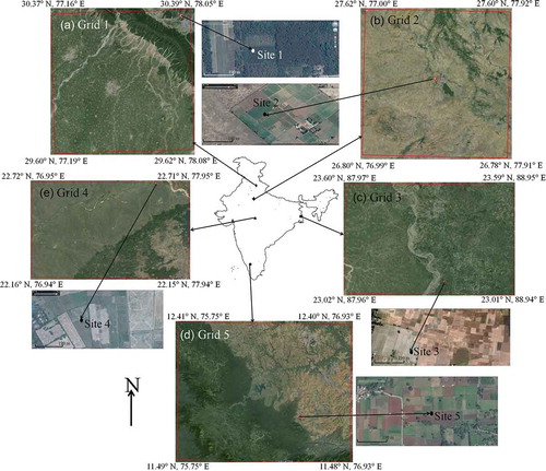
Figure 2. Land-use map of Grid 5, chosen for the spatial comparison of latent heat flux (Source: Bhuvan data portal, NRSC, ISRO).

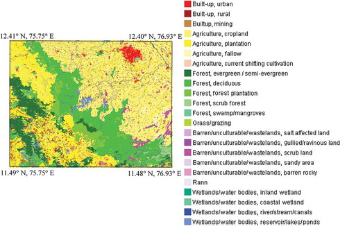
Figure 3. Annual (a) rainfall climatology and (b) elevation of Grid 5.

2.2 In situ data

The ground data required for comparing the three different λE models were obtained from the network of micrometeorological BREB towers conceived and installed by the Space Applications Centre of the Indian Space Research Organisation. The towers are 10 m in height. Three platinum resistance thermometers and capacitive-type hygrometers are installed at 2, 4 and 6 m above ground level to measure air temperature and relative humidity, respectively. Wind speed and wind direction are measured using cup anemometers and wind vanes, respectively, installed at 2.5, 5 and 10 m heights. The different components of surface radiation are measured using Kipp and Zonen four-component net radiometers (CNR-1 or CNR-4 type) mounted at 3 m above the ground. Two soil heat-flux plates are installed at 0.15 and 0.3 m below the surface and atmospheric pressure is measured at 2 m above ground level (a.g.l.) using a transducer. In addition to these instruments, the BREB tower has a raingauge (at 1 m a.g.l.) and a shaded pyranometer (at 4 m a.g.l.) for diffuse radiation measurement. Three soil thermometers and tensiometers to measure soil temperature and soil suction head, respectively, are installed at 0.05, 0.15 and 0.3 m below the surface. All the measured variables are sampled every 5 min and the 5-min samples are averaged at half-hourly intervals. The half-hourly averages are stored in a data logger and also transmitted to the server of the Space Applications Centre located at Ahmedabad in India.

2.3 Satellite data

The satellite data required for the three RS-based λE models were obtained from the MODIS sensors aboard the Terra and the Aqua satellites. The datasets used in this study are the daily land surface temperature and emissivity (MOD11A1/MYD11A1) at 1000 m resolution, daily seven-band surface reflectance at 500 m resolution (MOD09GA/MYD09GA), level-2 atmospheric profile product (MOD07_L2/MYD07_L2) at 5000 m resolution and yearly land-cover product (MCD12Q1) at 500 m resolution. All the datasets used in this study were acquired during the daytime pass of the satellite (Terra/Aqua). Information about the number of datasets acquired per BREB site and the period of data acquisition is provided in Table 2, and the data layers used in this study from each MODIS product are presented in Table 3. Apart from MODIS data, the elevation information was obtained from the Advanced Spaceborne Thermal Emission and Reflection Radiometer–Global Digital Elevation Model (ASTER-GDEM).

Table 2. Details on the MODIS datasets acquired for the study.

Location	MODIS sinusoidal tile number	Period of data acquisition	Number of datasets
			Terra	Aqua
Site 1	h24v05 h24v06	September 2010 to November 2010	36	23
Site 2	h24v06	March 2010 to April 2011	35	19
Site 3	h26v06	October 2010 to January 2011	23	12
Site 4	h25v06	January 2011 to March 2011	21	21
Site 5	h25v07	March 2012 to August 2013	28	30

Table 3. Information on the various MODIS data layers used in the study.

MODIS product	Layers	Spatial resolution (m)
MOD11A1/MYD11A1	Land surface temperature	1000
	Surface emissivity	1000
	Satellite view time	1000
MOD09GA/MYD09GA	Surface reflectance (7 bands)	500
	Solar zenith angle	1000
MOD07_L2/MYD07_L2	Air temperature	5000
	Dew point temperature	5000
MCD12Q1	Yearly land-cover (IGBP classification)	500

3 Methodology

3.1 Overview of estimation of λE from satellite data

The RS data provide only a snapshot of the Earth surface at the instant of satellite overpass. Due to this, the models (e.g. TSEB, Sim-ReSET) that estimate λE based on the surface energy balance equation provide the instantaneous value of latent heat flux at the time of satellite overpass (λE_inst) as their output. This instantaneous value is temporally upscaled using some reference scaling variable X, as given by (Cammalleri et al. 2014):

(1)

where the subscripts “inst” and “day” indicate, respectively, the instantaneous and daytime integrated values of the corresponding variables; and X can be any variable, such as: net available energy at the surface [(R_n – G), where R_n is the net radiation and G is the soil heat flux, W m⁻²]; global incoming solar radiation (R_global, W m⁻²); and reference evapotranspiration (Van Niel et al. 2012, Tang et al. 2013, Cammalleri et al. 2014). The most widely used reference variable is (R_n − G), and when it is substituted in place of X in Equation (1), we obtain:

(2)

(3)

where EF is the evaporative fraction, which is defined as the ratio of λE to the sum of sensible and latent heat fluxes (Shuttleworth et al. 1989). The EF estimated at the instant of satellite overpass is assumed to be constant for the whole daytime (Crago 1996) and is multiplied by (R_n – G)_day to obtain λE_day. Models such as the triangle and the S-SEBI yield EF directly, which can be converted to λE_day using Equation (3).

3.2 Description of the models

3.2.1 The triangle model

The triangle model is based on the inverse relationship between T_Rad and a vegetation index (VI), such as the NDVI or fraction of vegetation cover (f_veg). This inverse relationship between T_Rad and VI has been utilized for different applications in numerous studies for a long time (e.g. Nemani and Running 1989, Prihodko and Goward 1997). Jiang and Islam (1999) developed the triangle model for the estimation of EF and subsequently λE over the Southern Great Plains in the USA. Later this model was further tested at different sites across the globe by Jiang and Islam (2001), Venturini et al. (2004), Batra et al. (2006), Tang et al. (2010, 2011a), Laxmi and Nandagiri (2014) and Lu et al. (2015). In addition, the model was used to develop an operational λE product over southern Florida, USA, by Jiang et al. (2009). Long et al. (2012) highlighted that, when using the triangle model, the remotely sensed T_Rad data may not be able to detect the completely wet or dry pixels over the entire range of NDVI/f_veg in a given satellite scene owing to the absence of the extreme surface conditions in the region, or due to the spatially integrated nature of satellite observations; hence they developed a model to derive theoretical dry and wet edges based on the surface energy balance equation. The triangle model for the estimation of EF was tested at four sites in India (with RMSE of 0.09) by Eswar et al. (2013). The triangle model had undergone several modifications, such as using difference in T_Rad acquired on two different instances in a day (Wang et al. 2006, Stisen et al. 2008) and utilizing different vegetation indices in place of NDVI or f_veg (Kim and Hogue 2013, Tomas et al. 2014). In this model, the EF is formulated based on the Priestley-Taylor equation:

(4)

where is a complex surface parameter that can be thought of as a surrogate to surface and aerodynamic resistances (Jiang and Islam 1999); Δ is the slope of the saturated vapour pressure curve (hPa °C⁻¹) and γ is the psychrometric constant (hPa °C⁻¹). The spatial variation of is estimated from the T_Rad–NDVI context space, the schematic of which is shown in Figure 4.

In Figure 4, the segment is called the dry edge, along which λE happens at minimal rate, and the segment is called the wet edge, along which λE occurs at potential rate. At point A, where the dry edge intersects with NDVI = 0, λE is assumed to be zero, and hence ϕ is given a value of 0. However, ϕ = 1.26 (ϕ_max) at point B, where the dry and wet edges intersect. Further, ϕ is assumed to be linearly decreasing from B to A. Since λE occurs at potential rate along the segment , ϕ is fixed at 1.26 all along the segment. It is to be noted that the wet and dry edges may intersect within NDVI ≤ 1, giving the T_Rad–NDVI context space a triangular shape, and the point B will be in the range 0 ≤ NDVI ≤ 1. When the dry and wet edges do not intersect within NDVI ≤ 1, point B will be found when NDVI > 1 and the context space will have a trapezoidal shape (AB′B″C). This trapezoidal shape indicates the presence of water stress even for highly vegetated pixels (Long et al. 2012). Yang and Wang (2011) assumed ϕ to take an arbitrary value of 0.63 at point B′ for their site in the Southern Great Plains, and Laxmi and Nandagiri (2014) scaled ϕ_max based on the T_Rad – f_veg context space to explicitly estimate the value of ϕ at B′. In this study, the value of NDVI at point B (NDVI′, with NDVI′ ≤ 1 for triangular context space and NDVI′ > 1 for trapezoidal context space) was estimated numerically, and the minimum value of ϕ for a given value of NDVI (ϕ_min[NDVI]) was estimated using linear interpolation between ϕ_min = 0 at NDVI = 0 and ϕ_max = 1.26 at NDVI = NDVI′. This method was adopted because of its applicability to both triangular and trapezoidal context spaces. Further, if the T_Rad–NDVI context space has a trapezoidal shape, a reasonable value of ϕ_min at B′ can be estimated automatically without having to define it explicitly as in previous studies (Yang and Wang 2011, Laxmi and Nandagiri 2014). Then the value of ϕ for each pixel i, ϕ[i], was estimated using:

(5)

where is the maximum temperature for the value of NDVI (as defined by the dry edge) of pixel i; is the temperature corresponding to the wet edge; and T_Rad[i] is the land surface temperature for that particular pixel. The dry edge was determined using the algorithm proposed by Tang et al. (2010) and the wet edge was defined as the minimum land surface temperature at the maximum NDVI found in the satellite scene (Jiang and Islam 1999). The slope of the saturated vapour pressure curve, Δ, and γ were estimated using:

(6)

(7)

(8)

(9)

(10)

where e_s is the saturated vapour pressure (hPa), T_air is the air temperature (°C), P is the atmospheric pressure (hPa), C_P is the specific heat capacity of dry air at constant pressure (J kg⁻¹ °C⁻¹), λ is the latent heat of vaporization (J kg⁻¹) and h is the surface elevation (m). Equation (9) is used to account for the variation of λ with air temperature.

3.2.2 The S-SEBI model

The S-SEBI model is another contextual model for the estimation of EF and is based on the T_Rad–surface broadband albedo (α) contextual relationship (Roerink et al. 2000). Similarly to the triangle model, the S-SEBI model has also been tested and used in a large number of studies across the globe, such as Gomez et al. (2005), Sobrino et al. (2005, 2007), Mallick et al. (2009), Bhattacharya et al. (2010), Galleguillos et al. (2011a, 2011b), Li et al. (2012) and Guerra et al. (2014). In addition, Verstraeten et al. (2005) tried to develop an operational procedure for instantaneous λE estimation over the European continent, with emphasis on forest stands, using the S-SEBI model with data from AVHRR (Advanced Very High Resolution Radiometer) sensors.

Unlike the triangle model, the T_Rad–α context space does not have any characteristic shape on its own and it depends on the surface characteristics (Fig. 5). In Figure 5, segment is called the dry edge, along which λE is assumed to be zero, and all the (R_n – G) available at the surface is converted into sensible heat flux (H). However, segment is referred to as the wet edge, where all the (R_n – G) available at the surface is converted into λE with H assumed to be zero. For any pixel i in the satellite scene, EF from the T_Rad–α context space is given by:

(11)

where is the maximum temperature for a particular value of α (as defined by the dry edge) and is the minimum temperature for a particular value of α (as defined by the wet edge). Mallick et al. (2009) provided a detailed description of the T_Rad–α context space. The dry and wet edges were derived in an automated manner using the SPLIT method, as explained in Verstraeten et al. (2005), after the removal of outliers in T_Rad using the iterative approach described in Tang et al. (2010). Though Tang et al. (2010) developed the algorithm for automatic determination of the dry edge in the triangle model, the algorithm was found robust in removing outliers even when applied to the S-SEBI model after suitable modifications.

Figure 4. Schematic of the T_rad–NDVI triangle for the estimation of EF.

Figure 5. Schematic of the T_rad–surface albedo context space for the estimation of EF.

3.2.3 Estimation of daytime net available energy at the surface

To convert the EF estimated by the triangle and S-SEBI models to λE_day, the daytime integrated net available energy (R_n − G)_day was estimated independently. First (R_n)_inst was obtained by estimating each of its components at the instant of satellite overpass:

(12)

where R_global is the incoming global solar radiation, ε_s and ε_a are the broadband thermal emissivity for surface and air, respectively, and σ is the Stefan-Boltzmann constant (5.67 × 10⁻⁸ W m⁻² K⁻¹). Two sets of equations, one from Mallick et al. (2009) and the other from Bisht et al. (2005), were tested for estimating R_global and ε_a in Equation (11) (Table 4). Then, the instantaneous ground heat flux G, was estimated by:

(13)

The instantaneous values were converted into daytime integrated values using a sinusoidal model (Bisht et al. 2005):

(14)

where t_pass, t_rise and t_set are the times corresponding to satellite overpass, sunrise and sunset, respectively. It is to be noted that the equations in Table 4 and Equation (13) assume cloud-free conditions at the time of satellite pass. Further, Equation (14) also assumes the whole daytime to be cloud free.

Table 4. Equations used for estimation of (R_n – G)_inst.

Variable	Set 1 (Mallick et al. 2009)	Set 2 (Bisht et al. 2005)
Rglobal	a = 0.75 (empirical coefficient) b = 1.28 (empirical coefficient) S0: solar constant (1367 W m^–2) θ: solar zenith angle (radians) f: Sun–Earth distance correction factor (AU) dn: day of the year	τ: atmospheric transmissivity e0: vapour pressure (hPa) λ: latent heat of vaporization (see Equation (8)) Rv: gas constant for water vapour (461 J kg^−^1 K^−^1) Tdew: dew point temperature (°C)
εa		w: precipitable water content (g cm^–2)

3.2.4 The Sim-ReSET model

The physically-based single-pixel models such as TSEB and SEBS require different ground measurements (e.g. crop height, meteorological variables) as inputs. Sun et al. (2009) developed the Sim-ReSET model, which was formulated to work based on only RS data. The model was first tested using ground measurements alone at the Yucheng ecological station in North China, and was found to estimate instantaneous values of latent heat flux (λE_inst) with RMSE of 42 W m⁻² in comparison with eddy covariance measurements. Later, the Sim-ReSET model was further tested (Sun et al. 2013) with only MODIS datasets as inputs and the RMSE of the 16-day integrated λE_inst was in the range of 50–71 W m⁻² when compared with eddy tower measurements at five sites in China. The Sim-ReSET model is a two-source model that estimates the λE_inst of a single pixel as a combination of evapotranspiration from vegetation and bare soil :

(15)

where f_veg is the fraction vegetation cover. The individual components of Equation (14) were estimated as follows:

(16)

(17)

where z is the reference height above ground level (m) and A is the height of the upper boundary of the atmospheric surface layer (m). The superscripts “veg” and “soil” in Equations (16) and (17) indicate the values of the particular variables for vegetation and soil components of a pixel, respectively. Furthermore, the superscript “dry” on any variable indicates the value estimated over a reference dry bare soil surface. The terms d₀, z_0h and z_0m denote, respectively, the zero plane displacement height (m), roughness length for heat transfer (m) and roughness length for momentum transfer (m). For vegetated surfaces, these variables (d₀, z_0h and z_0m) were estimated from canopy height, which is, in turn, derived from a lookup table relating canopy height with land-cover type (International Geosphere-Biosphere Programme, IGBP classification). Derivations of Equations (16) and (17) can be found in Sun et al. (2009), and the detailed methodology for using MODIS datasets to solve the above equations is given in Sun et al. (2013). Since this study aims to compare λE_day estimated from three models, the λE_inst from the Sim-ReSET model was scaled up using Equations (2), (3) and (14). The (R_n – G)_inst in Equations (2) and (14) was estimated from the Sim-ReSET model using (Nishida et al. 2003):

(18)

Though the Sim-ReSET model was actually developed as a single-pixel model, when forcing the model with only RS-based inputs, it becomes necessary to estimate some variables such as and using the T_Rad–NDVI context space.

3.3 Satellite data processing

In this study, λE_day was estimated at a spatial resolution of 1000 m, as most of the primarily required MODIS datasets are available only at that resolution. The area pertaining to grids 1–5 (Fig. 1) was extracted from the MODIS tiles. The values of T_Rad, t_pass and surface emissivities at bands 31 and 32 were also extracted from the MOD11A1/MYD11A1 product. The narrow band emissivities were converted into surface broadband emissivity (ε_s) following Jin and Liang (2006). The seven-band surface reflectances from the MOD09GA/MYD09GA product at 500-m spatial resolution were re-sampled to 1000 m. The NDVI was estimated from the first two bands of the re-sampled surface reflectance data, and the surface broadband albedo (α) was estimated from the seven-band reflectances using the conversion formula given by Liang (2000). The air and dew-point temperatures (T_air and T_dew, respectively) were extracted from the MODIS atmospheric profile product from the vertical pressure level corresponding to the surface pressure level of the pixel. Furthermore, T_air and T_dew at 5000-m resolution were assumed to be uniform for all the 1000-m pixels within a single 5000-m pixel. Land-cover information required by the Sim-ReSET model was obtained from the MODIS yearly land-cover product (MCD12Q1).

3.4 In situ data processing

The estimation of λE_day from ground observations was carried out using the Bowen ratio energy balance method (Todd et al. 2000, Peacock and Hess 2004, Gavilan and Berengena 2007). The micrometeorological observations were checked for consistency and any anomalous and missing data points were excluded. Air temperature and relative humidity measured at two different heights were used to estimate the Bowen ratio (β). When the crop height in the catch of the tower was less than 2 m, measurements at 2 and 4 m were used, and when the crop height was greater than 2 m, measurements at 4 and 6 m were used. The value of β was estimated every half hour and subjected to the checks prescribed by Perez et al. (1999). This half-hourly β was further averaged during the entire daytime to obtain the daytime-averaged Bowen ratio (β_day). In this study, daytime was defined as the period during which the net shortwave radiation was positive. The daytime-averaged EF was estimated as 1/(1 + β_day). This daytime-averaged EF was used to validate the EF estimated from satellite data. Similarly, using the measurements from the four-component net radiometer and soil heat flux plates, (R_n – G) was estimated at half-hourly intervals and averaged over the entire daytime to obtain (R_n – G)_day. Daytime-averaged EF was estimated only on days when more than 70% of the data were available during the daytime period. Finally, the daytime averaged EF was multiplied by (R_n – G)_day to obtain λE_day from ground measurements.

4 Results and discussion

4.1 Validation of satellite-estimated EF

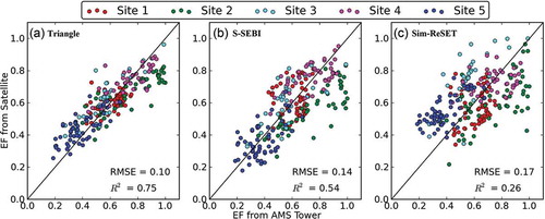
The EF estimated by the triangle, S-SEBI and Sim-ReSET models was compared with the EF estimated from ground data, and the comparison is presented in Figure 6. From Figure 6 it can be observed that the EF estimated using the triangle model had better performance in comparison with the other two models, with RMSE of 0.10 (16% of observed mean EF), 0.14 (23%) and 0.17 (28%) for the triangle, S-SEBI and the Sim-ReSET models, respectively, when data from all the five sites were taken together. Similarly, the bias was 0.001 (~0%), 0.04 (7%) and 0.18 (30%) for the three models considered in the same order. The results for individual sites are presented in Table 5. It can be observed from Table 5 that the EF from the triangle model had the lowest RMSE and the Sim-ReSET model had the highest RMSE at each of the five sites. The S-SEBI model also performed quite satisfactorily at all the five sites, however with a slightly higher RMSE than the triangle model.

Table 5. Results of comparison between EF estimated from satellite and from ground measurements.

Site	RMSE^a			Bias^b
	Triangle	S-SEBI	Sim-ReSET	Triangle	S-SEBI	Sim-ReSET
Site 1	0.08	0.12	0.13	–0.008	0.001	−0.03
Site 2	0.14	0.21	0.21	−0.08	−0.17	−0.13
Site 3	0.09	0.12	0.22	0.06	0.04	0.18
Site 4	0.08	0.10	0.13	−0.002	0.03	−0.008
Site 5	0.09	0.10	0.18	0.05	−0.02	0.16

^a

^b, where n is the total number of satellite datasets. Similar formulae were used to estimate RMSE and bias for (R_n – G)_day and λE_day.

Figure 6. Comparison of EF estimated from satellite using (a) triangle, (b) S-SEBI and (c) Sim-ReSET models with EF estimated from AMS tower data.

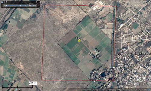
For the triangle and S-SEBI models, while Sites 1, 3, 4 and 5 had a comparable RMSE, Site 2 had a marginally higher RMSE and bias, with all the three satellite-based models underestimating EF in relation to ground measurements (Table 5). In order to find reason for this higher error at Site 2, the fetch area of the AMS tower and the area covered by the MODIS pixel enclosing the AMS site were compared. While the micrometeorological tower at Site 2 was located inside a farm with irrigation facilities, cultivating mustard, the MODIS pixel covers a large area of barren surface, as shown in Figure 7. In Figure 7, the MODIS pixel at 1000-m resolution is marked as a red square and the AMS tower is represented with a yellow “pin” marker. About 45% of the area of the MODIS pixel is covered by the farm and the remaining 55% is non-cropped area. The fetch of the tower will be much smaller and be completely under the irrigated farmland when compared with the MODIS pixel. Of the 54 datasets analysed for Site 2, 41 covered the cropping period (July–February) and the remaining 13 were obtained during the non-cropped period.

Figure 7. Google Earth^TM image showing the 1000-m MODIS pixel at Site 2 and the relative area of cropped and non-cropped land.

The error estimates for the cropped and non-cropped cases for Site 2 are presented in Table 6. From Table 6, it can be observed that the RMSE and bias of the MODIS EF with respect to the ground EF was relatively large for the cropped period, in comparison with the non-cropped period. The EF from the satellite was underestimated more during the cropped period than the non-cropped period. This suggests that the difference in the land cover of the MODIS pixel and the fetch area of the micrometeorological tower may be considered as the primary reason for higher RMSE and bias at Site 2 (e.g. Li et al. 2008).

Table 6. Results of comparison between satellite-estimated EF and ground-measured EF at Site 2 for cropped and non-cropped periods.

	RMSE			Bias
	Triangle	S-SEBI	Sim-ReSET	Triangle	S-SEBI	Sim-ReSET
Cropped	0.14	0.22	0.22	–0.10	−0.19	−0.14
Non-Cropped	0.10	0.11	0.14	0.05	−0.06	−0.02

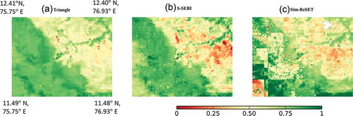
The spatial pattern of EF estimated by the three models was analysed for a particular day (14 November 2012) during the winter cropping season (Fig. 8). The EF estimated using the triangle (Fig. 8(a)) and the S-SEBI (Fig. 8(b)) models present a similar spatial pattern, with relatively higher values over forest areas and croplands adjacent to the Kabini River (see Fig. 8 with reference to Figs 2 and 3 for a clear picture on the spatial pattern). The agricultural areas in the western part of the basin (humid zone) mostly have plantations and hence they showed much higher EF than the agricultural plots in the eastern part (semi-arid zone) of the basin. The major difference between the triangle and S-SEBI models occurred at the eastern part of the basin, with the S-SEBI model estimating relatively lower EF than the triangle model. In contrast to these two models, the EF estimated using the Sim-ReSET model (Fig. 8(c)) could not properly capture the spatial patterns of the EF and presented a boxy appearance over the humid zone. On the basis of RMSE, bias, R² (Fig. 6) and spatial pattern, the triangle method was found to be the best performing model for the estimation of EF, followed by the S-SEBI model. The Sim-ReSET model did not capture the spatial patterns of EF properly and, further, had higher RMSE values.

Figure 8. Spatial pattern of EF derived from MODIS sensor on Aqua satellite using (a) the triangle model, (b) the S-SEBI model and (c) the Sim-ReSET model over Grid 5 on 14 November 2012. White patch in (c) indicates no value.

4.2 Comparison of satellite estimated (R_n – G)_day

The two models given by Mallick et al. (2009) and Bisht et al. (2005) for the estimation of (R_n − G)_day were compared with ground estimates. In addition, (R_n − G)_day was also estimated from the Sim-ReSET model. Hence, a total of three models for the estimation of daytime integrated net available energy were compared in this study. When data from all the five study sites were considered together, the RMSE in the satellite-derived (R_n − G)_day was, respectively, 29 W m⁻² (11% of the mean observed R_n − G), 40 W m⁻² (15%) and 60 W m⁻² (22%) for the Mallick et al. (2009), Bisht et al. (2005) and Sim-ReSET models. Similarly, the bias in satellite-modelled radiation was 0.94 W m⁻² (~0%), 24 W m⁻² (9%) and 23 W m⁻² (8%) for the three models taken in the same order. Scatter plots showing the evaluation of satellite-derived (R_n − G)_day with that measured using the AMS towers are presented in Figure 9.

The results for individual sites are presented in Table 7. From Table 7, it can be observed that the (R_n – G)_day estimated using the Sim-ReSET model had relatively larger RMSE than the Mallick et al. (2009) approach at all the five sites. Further, the Bisht et al. (2005) approach also had relatively much higher RMSE and bias than the Mallick et al. (2009) approach at Sites 3 and 4.

Table 7. Results of comparison between (R_n – G)_day estimated from satellite with that measured using ground data.

Site	RMSE (W m^−2)			Bias (W m^−2)
	Mallick et al. (2009)	Bisht et al. (2005)	Sim-ReSET	Mallick et al. (2009)	Bisht et al. (2005)	Sim-ReSET
Site 1	30	28	40	−21	10	14
Site 2	23	31	33	2	15	4
Site 3	40	67	96	38	64	92
Site 4	27	49	82	14	44	77
Site 5	25	28	50	−10	9	−30

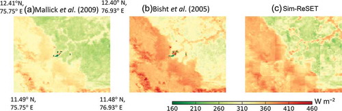
The spatial pattern of (R_n – G)_day estimated using the three models is presented in Figure 10. The highest value of (R_n – G)_day was found along the evergreen/semi-evergreen forests in the basin (humid zone), followed by the deciduous forests in the middle portion of the image (transition zone). The agricultural lands with plantations had a higher net available energy than the croplands. The approach proposed by Bisht et al. (2005) (Fig. 10(b)) had relatively higher values of (R_n – G)_day than the Mallick et al. (2009) approach (Fig. 10(a)). The Sim-ReSET model also captured the spatial pattern of net available energy quite satisfactorily. The spatial pattern of (R_n – G)_day estimated from the Sim-ReSET model matched that of the Bisht et al. (2005) approach for the humid and transition zones, and the patterns matched the Mallick et al. (2009) approach for the semi-arid zones. However, some boxy artefacts were noted in the radiation estimated from the Sim-ReSET model. On the basis of RMSE, bias and R² (Fig. 9), the approach of Mallick et al. (2009) was found to be the best performing model among the three tested for the estimation of (R_n – G)_day.

Figure 9. Comparison of (R_n – G)_day estimated from satellite using (a) the Mallick et al. (2009) approach, (b) the Bisht et al. (2005) approach and (c) the Sim-ReSET model, with (R_n – G)_day measured at AMS tower sites.

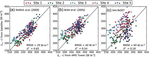
Figure 10. Spatial pattern of (R_n – G)_day derived from MODIS sensor on Aqua satellite using (a) the Mallick et al. (2009) approach, (b) the Bisht et al. (2005) approach and (c) the Sim-ReSET model over Grid 5 on 14 November 2012.

4.3 Comparison of satellite estimated λE_day

Since the radiation estimated by the Mallick et al. (2009) approach was found to be better performing, the (R_n – G)_day estimated by that model was combined with the EF from the triangle and S-SEBI models to obtain λE_day. In addition, λE_day from the Sim-ReSET model was also generated using EF and (R_n – G)_day generated by that model itself. The RMSE of the λE_day was, respectively, 34 W m⁻² (17% of observed mean λE_day), 41 W m⁻² (20%) and 68 W m⁻² (34%) for the triangle-based, S-SEBI-based and Sim-ReSET models respectively. Similarly, the bias in the satellite estimated λE_day was 2 W m⁻² (1%), –7 W m⁻² (−4%) and 27 W m⁻² (14%) for the three models considered in the same order as above. The error estimates for individual sites are presented in Table 8. The relatively higher errors in the estimation of EF and (R_n – G)_day, respectively, at Sites 2 and 3 propagated into the estimated λE_day at those sites. While the λE_day at Site 2 was underestimated compared to ground measurements due to underestimation of EF, it was overestimated at Site 3 due to overestimation of (R_n – G)_day. As expected, the Sim-ReSET model performance was inferior to that of the other models in estimating λE_day as it performed poorly in estimating both EF and (R_n – G)_day.

Table 8. Results of comparison between λE_day estimated from satellite with that measured using ground data.

Site	RMSE (W m^−2)			Bias (W m^−2)
	Triangle + Mallick et al. (2009)	S-SEBI + Mallick et al. (2009)	Sim-ReSET	Triangle + Mallick et al. (2009)	S-SEBI + Mallick et al. (2009)	Sim-ReSET
Site 1	33	39	52	−15	−15	2
Site 2	39	52	57	−17	−40	−26
Site 3	44	46	119	38	30	111
Site 4	30	36	68	9	17	52
Site 5	25	30	47	12	−10	34

The spatial patterns of λE_day estimated by the three models are presented in Figure 11. Higher latent heat flux was observed at humid zones with evergreen/semi-evergreen forests followed by the deciduous forest in the transition zone. The croplands in the semi-arid zone had lower values of λE_day in comparison with plantations in the humid zone. As mentioned before for EF and (R_n – G)_day, the relatively simpler models performed better than the dual-source Sim-ReSET model in capturing the spatial pattern of λE_day. The dual-source Sim-ReSET model has a lot of variables, parameters and assumptions involved in it. The estimation of those variables and parameters only from the remote sensing datasets might have caused higher errors in the performance of the model. Sun et al. (2009) have shown that the Sim-ReSET model yielded better results when driven with ground-based measurements. However, in most regions across the globe, the requirement of ground data for model parameterization will limit the model’s applicability. The boxy appearance in the EF and (R_n – G)_day estimated from the Sim-ReSET model was due to the estimation of the soil, vegetation and reference dry bare surface components of T_rad using the T_rad–NDVI context space by running a 20 km × 20 km moving window (Sun et al. 2013) across the image. Long et al. (2012) demonstrated that the T_rad–NDVI is defined properly when working over spatial domains with area in the order of 10⁴ km². This suggests that there may not be enough spatial variation in soil moisture within each of the 20 km × 20 km (400 km² area) moving windows and, hence, the T_rad–NDVI context space might not have resolved properly. This improper determination of T_rad–NDVI context space will introduce higher uncertainty in estimating different components of land surface temperature, which will further affect the estimated λE.

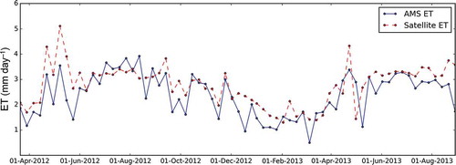
In order to further verify the performance of the triangle model, the temporal evolution of evapotranspiration (ET, latent heat flux expressed in volume units, i.e. mm d⁻¹) estimated from the triangle model was compared with the AMS ET at Site 5 (Fig. 12). In Figure 12, to reduce the complexity of the plot, 8-day averaged ET is presented instead of daily values. Further, any gaps in the 8-day ET estimated from the satellite are filled with ET estimated from meteorological data for the completeness of the plot. From Figure 12, it can be observed that relatively higher ET occurs during the month of May due to the pre-monsoon rainfall and agricultural activities. The ET remains in the range of 3–4 mm d⁻¹ during the primary cropping season between June and mid-September, and gradually reduces during October. Again, with the beginning of the second cropping season in mid-October, ET increases and remains in the range of 2–3 mm d⁻¹. After mid-January, when the majority of the crops are harvested, ET falls below 2 mm d⁻¹ and remains low till the next cropping season. The satellite-estimated ET captured this seasonal pattern reasonably well, especially during the two cropping seasons. However, a small overestimation of ET was observed during the non-cropping periods.

Figure 11. Spatial pattern of λE_day derived from MODIS sensor on Aqua satellite over Grid 5 on 14 November 2012. λE_day estimated using the (a) triangle and (b) S-SEBI models with (R_n – G)_day estimated following the Mallick et al. (2009) approach. (c) λE_day estimated using the Sim-ReSET model. White patch in (c) indicates no value.

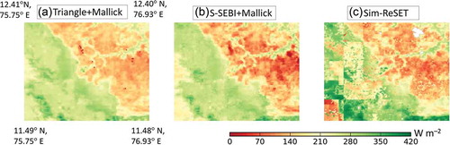
Figure 12. Time series of ground-measured and satellite-estimated ET at Site 5.

5 Conclusion

This study compared the different models for the estimation of daytime latent heat flux (λE_day) from satellite datasets alone. The λE_day was estimated as a product of EF and daytime integrated net available energy, (R_n – G)_day. Two contextual models, the triangle model and the S-SEBI model, were tested for the estimation of EF. For estimating the (R_n – G) required to convert EF into λE, two simple clear-sky models proposed by Mallick et al. (2009) and Bisht et al. (2005) were tested. Apart from semi-empirical models, a more physically-based two-source model known as the Sim-ReSET was also chosen for the study. The models were tested at five sites in India using data from Bowen ratio towers. The study showed that the simple context-based models yielded more accurate λE_day than the physically-based model when the models were driven only with RS-based inputs and in the absence of any ground data. Considering the better performance of the triangle model, it is envisaged to use the model for developing a satellite-based ET product over India.

Disclosure statement

No potential conflict of interest was reported by the authors.

Additional information

Funding

The first author acknowledges the fellowship provided by the Department of Science and Technology, Government of India, under the INSPIRE fellowship programme (IF110547) for his doctoral studies. This study was carried out with partial funding from the IISc-ISRO STC project titled “Modelling evapotranspiration from remote sensing” [grant number ISTC/MCV/MS/351] and from the SAC-ISRO project “Calibration and validation of SMAP soil moisture product over an experimental agricultural watershed in Karnataka”.

References

- Anderson, M.C., et al., 2012. Use of Landsat thermal imagery in monitoring evapotranspiration and managing water resources. Remote Sensing of Environment, 122, 50–65. doi:10.1016/j.rse.2011.08.025
- Batra, N., et al., 2006. Estimation and comparison of evapotranspiration from MODIS and AVHRR sensors for clear sky days over the Southern Great Plains. Remote Sensing of Environment, 103, 1–15. doi:10.1016/j.rse.2006.02.019
- Bhattacharya, B.K., et al., 2010. Regional clear sky evapotranspiration over agricultural land using remote sensing data from Indian geostationary meteorological satellite. Journal of Hydrology, 387, 65–80. doi:10.1016/j.jhydrol.2010.03.030
- Bisht, G., et al., 2005. Estimation of the net radiation using MODIS (Moderate Resolution Imaging Spectroradiometer) data for clear sky days. Remote Sensing of Environment, 97, 52–67. doi:10.1016/j.rse.2005.03.014
- Cammalleri, C., Anderson, M.C., and Kustas, W.P., 2014. Upscaling of evapotranspiration fluxes from instantaneous to daytime scales for thermal remote sensing applications. Hydrology and Earth System Sciences, 18, 1885–1894. doi:10.5194/hess-18-1885-2014
- Chirouze, J., et al., 2014. Intercomparison of four remote-sensing-based energy balance methods to retrieve surface evapotranspiration and water stress of irrigated fields in semi-arid climate. Hydrology and Earth System Sciences, 18 (3), 1165–1188. doi:10.5194/hess-18-1165-2014
- Crago, R.D., 1996. Conservation and variability of the evaporative fraction during the daytime. Journal of Hydrology, 180, 173–194. doi:10.1016/0022-1694(95)02903-6
- Eswar, R., Sekhar, M., and Bhattacharya, B.K., 2013. A simple model for spatial disaggregation of evaporative fraction: comparative study with thermal sharpened land surface temperature data over India. Journal of Geophysical Research-Atmospheres, 118, 12,029–12,044. doi:10.1002/2013JD020813
- Galleguillos, M., et al., 2011b. Comparison of two temperature differencing methods to estimate daily evapotranspiration over a Mediterranean vineyard watershed from ASTER data. Remote Sensing of Environment, 115, 1326–1340. doi:10.1016/j.rse.2011.01.013
- Galleguillos, M., et al., 2011a. Mapping daily evapotranspiration over a mediterranean vineyard watershed. IEEE Geoscience and Remote Sensing Letters, 8 (1), 168–172. doi:10.1109/LGRS.2010.2055230
- Gavilan, P. and Berengena, J., 2007. Accuracy of the Bowen ratio-energy balance method for measuring latent heat flux in a semiarid advective environment. Irrigation Science, 25, 127–140. doi:10.1007/s00271-006-0040-1
- Glenn, E.P., Nagler, P.L., and Huete, A.R., 2010. Vegetation index methods for estimating evapotranspiration by remote sensing. Surveys in Geophysics, 31 (6), 531–555. doi:10.1007/s10712-010-9102-2
- Gomez, M., et al., 2005. Retrieval of evapotranspiration over the Alpilles/ReSeDA experimental site using airborne POLDER sensor and a thermal camera. Remote Sensing of Environment, 96, 399–408. doi:10.1016/j.rse.2005.03.006
- Guerra, L.O., Mattar, C., and Galleguillos, M., 2014. Estimation of real evapotranspiration and its variation in Mediterranean landscapes of central-southern Chile. International Journal of Applied Earth Observation and Geoinformation, 28, 160–169. doi:10.1016/j.jag.2013.11.012
- Jiang, L. and Islam, S., 1999. A methodology for estimation of surface evapotranspiration over large areas using remote sensing observations. Geophysical Research Letters, 26 (17), 2773–2776. doi:10.1029/1999GL006049
- Jiang, L. and Islam, S., 2001. Estimation of surface evaporation map over southern great plains using remote sensing data. Water Resources Research, 37 (2), 329–340. doi:10.1029/2000WR900255
- Jiang, L., et al., 2009. A satellite-based Daily Actual Evapotranspiration estimation algorithm over South Florida. Global and Planetary Change, 67, 62–77. doi:10.1016/j.gloplacha.2008.12.008
- Jin, M. and Liang, S., 2006. An improved land surface emissivity parameter for land surface models using global remote sensing observations. Journal of Climate, 19, 2867–2881. doi:10.1175/JCLI3720.1
- Kim, J. and Hogue, T.S., 2013. Evaluation of a MODIS triangle-based evapotranspiration algorithm for semi-arid regions. Journal of Applied Remote Sensing, 7, 073493. doi:10.1117/1.JRS.7.073493
- Laxmi, K. and Nandagiri, L., 2014. Latent heat flux estimation using trapezoidal relationship between MODIS land surface temperature and fraction of vegetation–application and validation in a humid tropical region. Remote Sensing Letters, 5 (11), 981–990. doi:10.1080/2150704X.2014.984083
- Li, F., et al., 2008. Effect of remote sensing spatial resolution on interpreting tower-based flux observations. Remote Sensing of Environment, 112, 337–349. doi:10.1016/j.rse.2006.11.032
- Li, X., et al., 2012. Estimation of evapotranspiration in an arid region by remote sensing—A case study in the middle reaches of the Heihe River Basin. International Journal of Applied Earth Observation and Geoinformation, 17, 85–93. doi:10.1016/j.jag.2011.09.008
- Liang, S., 2000. Narrowband to broadband conversions of land surface albedo: I. Algorithms, Remote Sensing of Environment, 76, 213–238. doi:10.1016/S0034-4257(00)00205-4
- Long, D., Singh, V.P., and Scanlon, B.R., 2012. Deriving theoretical boundaries to address scale dependencies of triangle models for evapotranspiration estimation. Journal of Geophysical Research-Atmospheres, 117. doi:10.1029/2011JD017079
- Lu, J., et al., 2015. Assessment of two temporal-information-based methods for estimating evaporative fraction over the Southern Great Plains. International Journal of Remote Sensing, 36 (19–20), 4936–4952. doi:10.1080/01431161.2015.1040133
- Mallick, K., et al., 2009. Latent heat flux estimation in clear sky days over Indian agroecosystems using noon-time satellite remote sensing data. Agricultural and Forest Meteorology, 149 (10), 1646–1665. doi:10.1016/j.agrformet.2009.05.006
- Narasimhan, T.N., 2008. A note on India’s water budget and evapotranspiration. Journal of Earth System Science, 117 (3), 237–240. doi:10.1007/s12040-008-0028-8
- Nemani, R.R. and Running, S.W., 1989. Estimation of regional surface-resistance to evapotranspiration from NDVI and thermal-IR AVHRR data. Journal of Applied Meteorology, 1989 (28), 276–284. doi:10.1175/1520-0450(1989)028<0276:EORSRT>2.0.CO;2
- Nishida, K., et al., 2003. An operational remote sensing algorithm of land surface evaporation. Journal of Geophysical Research, 108 (D9), 4270. doi:10.1029/2002JD002062
- Norman, J.M., Kustas, W.P., and Humes, K.S., 1995. Source approach for estimating soil and vegetation energy fluxes from observations of directional radiometric surface temperature. Agricultural and Forest Meteorology, 77, 263–293. doi:10.1016/0168-1923(95)02265-Y
- Peacock, C.E. and Hess, T.M., 2004. Estimating evapotranspiration from a reed bed using the Bowen ratio energy balance method. Hydrological Processes, 18, 247–260. doi:10.1002/hyp.1373
- Perez, P.J., et al., 1999. Assessment of reliability of Bowen ratio method for partitioning fluxes. Agricultural and Forest Meteorology, 97, 141–150. doi:10.1016/S0168-1923(99)00080-5
- Prihodko, L. and Goward, S.N., 1997. Estimation of air temperature from remotely sensed surface observations. Remote Sensing of Environment, 60, 335–346. doi:10.1016/S0034-4257(96)00216-7
- Roerink, G.J., Su, Z., and Menenti, M., 2000. S-SEBI: a simple remote sensing algorithm to estimate the surface energy balance. Physics and Chemistry of the Earth, 25, 147–157. doi:10.1016/S1464-1909(99)00128-8
- Sekhar, M., et al., 2016. Influences of climate and agriculture on water and biogeochemical cycles: kabini critical zone observatory. Proceedings of Indian National Science Academy, 82 (3), 833–846. doi:10.16943/ptinsa/2016/48488
- Shuttleworth, W.J., et al., 1989. FIFE: the variation in energy partition at surface flux sites. IAHS Publications, 186, 67–74.
- Singh, V., 2015. The Indian critical zone – a case for priority studies. Current Science, 108 (6), 1045–1046.
- Sobrino, J.A., et al., 2007. Application of a simple algorithm to estimate daily evapotranspiration from NOAA–AVHRR images for the Iberian Peninsula. Remote Sensing of Environment, 110, 139–148. doi:10.1016/j.rse.2007.02.017
- Sobrino, J.A., et al., 2005. A simple algorithm to estimate evapotranspiration from DAIS data: application to the DAISEX campaigns. Journal of Hydrology, 315, 117–125. doi:10.1016/j.jhydrol.2005.03.027
- Stisen, S., et al., 2008. Combining the triangle method with thermal inertia to estimate regional evapotranspiration — applied to MSG-SEVIRI data in the Senegal River basin. Remote Sensing of Environment, 112, 1242–1255. doi:10.1016/j.rse.2007.08.013
- Su, Z., 2002. The surface energy balance system (SEBS) for estimation of turbulent heat fluxes. Hydrology and Earth System Sciences, 6 (1), 85–99. doi:10.5194/hess-6-85-2002
- Sun, Z., et al., 2009. Development of a simple remote sensing evapotranspiration model (Sim-ReSET): algorithm and model test. Journal of Hydrology, 376, 476–485. doi:10.1016/j.jhydrol.2009.07.054
- Sun, Z., et al., 2013. Further evaluation of the Sim-ReSET model for ET estimation driven by only satellite inputs. Hydrological Sciences Journal, 58 (5), 994–1012. doi:10.1080/02626667.2013.791026
- Tang, R., Li, Z.L., and Chen, K.S., 2011a. Validating MODIS - derived land surface evapotranspiration with in situ measurements at two AmeriFlux sites in a semiarid region. Journal of Geophysical Research-Atmospheres, 116. doi:10.1029/2010JD014543
- Tang, R., et al., 2011b. An intercomparison of three remote sensing-based energy balance models using Large Aperture Scintillometer measurements over a wheat–corn production region. Remote Sensing of Environment, 115, 3187–3202. doi:10.1016/j.rse.2011.07.004
- Tang, R., Li, Z.L., and Sun, X., 2013. Temporal upscaling of instantaneous evapotranspiration: an intercomparison of four methods using eddy covariance measurements and MODIS data. Remote Sensing of Environment, 138, 102–118. doi:10.1016/j.rse.2013.07.001
- Tang, R., Li, Z.L., and Tang, B., 2010. An application of the Ts–VI triangle method with enhanced edges determination for evapotranspiration estimation from MODIS data in arid and semi-arid regions: implementation and validation. Remote Sensing of Environment, 114, 540–551. doi:10.1016/j.rse.2009.10.012
- Todd, R.W., Evett, S.R., and Howell, T.A., 2000. The Bowen ratio-energy balance method for estimating latent heat flux of irrigated alfalfa evaluated in a semi-arid, advective environment. Agricultural and Forest Meteorology, 103, 335–348. doi:10.1016/S0168-1923(00)00139-8
- Tomas, A.D., et al., 2014. Validation and scale dependencies of the triangle method for the evaporative fraction estimation over heterogeneous areas. Remote Sensing of Environment, 152, 493–511. doi:10.1016/j.rse.2014.06.028
- Van Niel, T.G., et al., 2012. Upscaling latent heat flux for thermal remote sensing studies: comparison of alternative approaches and correction of bias. Journal of Hydrology, 468–469, 35–46. doi:10.1016/j.jhydrol.2012.08.005
- Venturini, V., et al., 2004. Comparison of evaporative fractions estimated from AVHRR and MODIS sensors over South Florida. Remote Sensing of Environment, 93, 77–86. doi:10.1016/j.rse.2004.06.020
- Verstraeten, W.W., Veroustraete, F., and Feyen, J., 2005. Estimating evapotranspiration of European forests from NOAA-imagery at satellite overpass time: towards an operational processing chain for integrated optical and thermal sensor data products. Remote Sensing of Environment, 96, 256–276. doi:10.1016/j.rse.2005.03.004
- Wang, K., Li, Z., and Cribb, M., 2006. Estimation of evaporative fraction from a combination of day and night land surface temperatures and NDVI: a new method to determine the Priestley – Taylor parameter. Remote Sensing of Environment, 102, 293–305. doi:10.1016/j.rse.2006.02.007
- Yang, J. and Wang, Y., 2011. Estimating evapotranspiration fraction by modeling two-dimensional space of NDVI/albedo and day–night land surface temperature difference: A comparative study. Advances in Water Resources, 34, 512–518. doi:10.1016/j.advwatres.2011.01.006