Data-based modelling approach for variable density flow and solute transport simulation in a coastal aquifer

ABSTRACT

Data-based models, namely artificial neural network (ANN), support vector machine (SVM), genetic programming (GP) and extreme learning machine (ELM), were developed to approximate three-dimensional, density-dependent flow and transport processes in a coastal aquifer. A simulation model, SEAWAT, was used to generate data required for the training and testing of the data-based models. Statistical analysis of the simulation results obtained by the four models show that the data-based models could simulate the complex salt water intrusion process successfully. The selected models were also compared based on their computational ability, and the results show that the ELM is the fastest technique, taking just 0.5 s to simulate the dataset; however, the SVM is the most accurate, with a Nash-Sutcliffe efficiency (NSE) ≥ 0.95 and correlation coefficient R ≥ 0.92 for all the wells. The root mean square error (RMSE) for the SVM is also significantly less, ranging from 12.28 to 77.61 mg/L.

KEYWORDS:

• salt water intrusion
• extreme learning machine (ELM)
• support vector machine (SVM)
• genetic programming (GP)
• artificial neural network (ANN)
• SEAWAT model

Editor R. Woods Associate editor F.-J. Chang

1 Introduction

Groundwater is the main source of water supply in many coastal regions and most of the aquifers in the coastal belt are overexploited due to an ever-increasing demand for water. Thus excessive pumping of groundwater gives rise to salt water intrusion (Rao et al. 2004). Under normal conditions, freshwater would flow into the sea; however, excessive abstraction of water may lead to reverse groundwater flow, thereby causing salt water intrusion (Bhattacharjya and Datta 2009). Salt water intrusion leads to an increase in the saline water volume and, correspondingly, a decrease in the freshwater volume (Langevin et al. 2005). Salinization of groundwater is very important because mixing even a small quantity of salt water (2–3%) with groundwater makes freshwater unsuitable for use and may result in abandonment of freshwater supply wells when salt concentration exceeds drinking water standards (Abd-Elhamid and Javadi 2011). Thus, salt water intrusion should be prevented or at least controlled to protect groundwater resources. Bear et al. (1999) suggest that uncontrolled abstraction of water from aquifers, or seasonal variations in parameters such as natural groundwater flow, barometric pressure, tidal effects, seismic waves, dispersion and climate change could result in salt water intrusion problems.

A review of the literature shows that various numerical models, such as SUTRA (Voss 1984), MOCDENS3D (Sanford and Konikow 1985), CODESA-3D (Lecca 2000), FEMWATER (Lin et al. 1997) and MODFLOW (Harbaugh et al. 2000), have been developed to simulate the salt water intrusion process. However, the SEAWAT model (Guo and Langevin 2002) has been successfully applied to simulate a variable-density fluid flow through complex geometries and geological settings. The SEAWAT model has been used to simulate seawater intrusion in coastal aquifers, submarine groundwater discharge, brine transport, and groundwater flow near salt domes (Rao et al. 2004, Langevin et al. 2005, Qahman and Larabi 2006, Schneider and Kruse 2006, Kourakos and Mantoglou 2009, 2013, Lin et al. 2009; Cobaner et al. 2012, Morgan et al. 2013, Chekirbane et al. 2015, Gopinath et al. 2016, Holding and Allen 2016, Vijay and Mohapatra 2016). Although numerical models have been used successfully to study the salt water intrusion phenomenon, Rao et al. (2004) suggested that applicability of complex numerical models such as SEAWAT in the simulation–optimization approach could increase the computational time significantly. Thus, the use of soft computing techniques as an approximation model could speed up the computation process while determining an optimal solution. The use of data-based models cannot be seen as an alternative to the numerical models; however, these models can be used to find a balanced outcome between the model complexities and solution accuracy (Rao et al. 2004). A simulation–optimization approach using data-based models in place of numerical models would require a sufficiently accurate proxy simulator (Bhattacharjya and Datta 2009). The data-based simulation approach also takes considerably less computational time when compared to numerical models.

The management strategy of salt water intrusion is based on simulation of flow and transport processes. Simulation of these processes becomes more complicated in coastal zones, in particular, due to density-dependent flow. Moreover, the coupling of the simulation model with optimization techniques makes simulation more complex and time consuming (Bhattacharjya and Datta 2009). Bhattacharjya et al. (2007) proposed an artificial neural network (ANN) model to simulate the density-dependent salt water intrusion process in coastal aquifers and suggested that the ANN can reduce the computational burden significantly without impairing the simulation accuracy. Similarly, Kourakos and Mantoglou (2009, 2013) used a modular neural networks-based virtual simulator to replace the complex numerical model (SEAWAT), and suggested that the surrogate model not only improves the simulation accuracy but also reduces the computational burden significantly. Following this, Sreekanth and Datta (2010, 2011, 2014) developed management strategies using data-based models to slow/prevent salt water intrusion in coastal areas, and the numerical model FEMWATER was used to generate the dataset for the training of the data-based models. The studies proposed genetic programming (GP) as a replacement for FEMWATER, and found that GP is better suited for optimization using an adaptive search method. Similarly, Banerjee et al. (2011) successfully used ANN to predict groundwater salinity of an island aquifer. In the same way, Ashtiani et al. (2013) proposed a combination of ANN and genetic algorithm (GA) to manage freshwater in small islands and suggested that the ANN could provide a more effective framework while minimizing seawater intrusion. Hussain et al. (2015) presented a surrogate modelling technique, evolutionary polynomial regression (EPR), for simulation of salt water intrusion, and successfully used it in a coupled simulation–optimization model to minimize the project costs. Roy and Datta (2017)used a Sugeno-type fuzzy inference system (FIS) replacing FEMWATER to predict salt water concentration at different monitoring locations, and suggested that FIS can simulate the complex physical processes of heterogeneous coastal aquifers.

The literature review thus indicates that data-based models can be used to simulate the salt water intrusion process accurately. It is also evident from the literature that only a few data-based models (ANN, GP, FIS) have been tested so far; however, research in the field of machine learning has shown that new and efficient models, such as support vector machine (SVM) (Vapnik 1995) and extreme learning machine (ELM) (Huang et al. 2004), have been developed very recently. These models have been used in various water quantity and quality problems and are able to overcome most of the shortcomings associated with the traditional models such as ANN and GP. The main advantage of a kernel-based method such as SVM is that it not only retains the strengths of the ANN but is able to overcome the problems associated with network overfitting and local minimum (ASCE Task Committee on Application of Artificial Neural Networks in Hydrology 2000). Although the SVM model has been successfully used in many areas (Lin et al. 2006, Yu et al. 2006, Wang et al. 2009, 2013, Nikam and Gupta 2013, Gizaw and Gan 2016), suitable selection of kernel function and associated parameters are crucial for accurate model output. The SVM parameters, such as regularization constant, insensitive loss function and parameter of radial basis function, are heuristic and are generally selected through a time-consuming trial-and-error process (Deka 2014).

Recently, Huang et al. (2006) proposed a data-driven algorithm for a single-layer feedforward neural network (SLFN), referred to as the extreme learning machine (ELM), that helps to reduce the computational time required for training a neural network. Studies using the ELM have attained very fast learning along with a good generalization performance due to the simplified training processes involved (Huang et al. 2004, Liang et al. 2006, Mohammadi et al. 2015; Shamshirband et al. 2015a). Application of the ELM model in different scientific areas, such as prediction of coal mine water inrush (Zhao et al. 2013), nonstationary time series prediction (Wang and Han 2014), estimation of monsoon rainfall (Acharya et al. 2014), estimation of wind speed distribution (Shamshirband et al. 2015b), and rainfall–runoff modelling (Taormina and Chau 2015), has been reported. Recently, Yadav et al. (2016b) compared the computational ability of the data-based models ANN, SVM and ELM, and suggested that the ELM model is the fastest and most accurate in simulating the target output in the in situ bioremediation of a polluted aquifer zone.

Data-based models have been used in salt water intrusion studies as a proxy simulator; however, their simulation accuracy can be improved by using new soft computing techniques such as SVM and ELM. A review of the literature shows that, although SVM and ELM have been used to simulate various natural phenomena, their application in salt water intrusion has not yet been explored. The focus of this study is to examine the suitability of SVM and ELM for the simulation of the salt water intrusion process, and to compare the results with already established ANN and GP methods. The data for the training and testing of the selected models were generated using SEAWAT, which is widely used to simulate variable density flow and solute transport processes. An illustrative study area was used to analyse the performance of the developed models.

2 Methodology

2.1 SEAWAT

The SEAWAT model is used to simulate salt water intrusion in a coastal aquifer. The software solves the coupled flow and solute-transport equations to simulate three-dimensional, variable-density, transient groundwater flow in porous media. It is assumed that the fluid density is solely a function of dissolved constituents concentration, and variation in fluid density with respect to temperature is not considered. Juster (1995) suggested the use of equivalent freshwater heads, which leads to a system of equations that an existing MODFLOW structure could solve easily. The gradient of freshwater heads allows the model to directly evaluate the horizontal flow components under variable-density flow conditions. The vertical component of the flow is considered using a buoyancy term or a relative density difference term similar in magnitude to the freshwater head (Holzbecher 1998, Oude Essink 1998, Guo and Langevin 2002). The dynamic viscosity is a weak function of solute concentration and is thus neglected during the modelling. The effect of temperature or pressure on fluid density has not been considered and hence is valid only in an isothermal system for an incompressible fluid. The development presented in this study also assumes that flow is laminar and a diffusive approach for the salt distribution is applicable. The porous medium is assumed to be fully saturated with water. For a detailed description of the SEAWAT model, readers are referred to Guo and Langevin (2002).

2.2 Illustrative study area

The hypothetical site of Dhar and Datta (2009) for a coastal aquifer of 2.52 km² area is adopted in the study (Fig. 1). The dimensions of the aquifers are 1800 m × 1400 m × 100 m and the boundary on the right is the ocean face. The grid size is 150 m × 155 m × 12.5 m for Δx × Δy × Δz, respectively. The flow and transport process for this grid was solved using a daily time step. In this study the aquifer is assumed to be homogeneous and isotropic, with the well-screen placed well below the ground surface. The confined aquifer system is subjected to salt water intrusion along the coastal side of the study area. On account of a hydraulic gradient, the salt water enters the well through this lower portion along the ocean face yielding a brackish environment. The aquifer system allows entry of freshwater through the left boundary (inland face). Except for the ocean and inland faces, all other sides of the aquifer are assumed to be impermeable with zero flux across them, thus the Dirichlet condition is taken as the flow boundary condition. Along the inland face, a linearly varying head is assigned with a value of 1.66 m near the front face, with 1.74 m at the back face. Seawater level is assumed to be constant in this analysis. The flow boundary condition on the ocean face is assigned a hydrostatic head value. The initial water level in the aquifer is at the ground surface.

Figure 1. Study area showing the plan view and sectional view (Dhar and Datta 2009).

Initially, the aquifer is assumed to have a zero concentration of solute throughout. The Dirichlet boundary conditions for concentrations along the inland and the ocean face are 0 and 35 000 mg/L, respectively. Along the remaining boundaries, the mass flux of concentration is assigned a zero value. All the boundaries are time invariant and the various parameters used for simulation are specified in Table 1. The simulation of salt water intrusion is conducted for five pumping wells (PW) and two observation wells (OW) located as shown in Figure 1. The pumping wells have been assigned a 10-m screen interval with top and bottom screens at –40 and –50 m, respectively. A single time period of 183 days is considered in the numerical model. The time step used for the simulation is much smaller; however, the pumping rates, which vary between 0 and 10 000 m³, are constant throughout the chosen time period of 183 days.

Table 1. List of aquifer parameters used for simulating the study area (Dhar and Datta 2009).

Parameter	Unit	Value
Hydraulic conductivity in x-direction	m/d	25
Hydraulic conductivity in y-direction	m/d	25
Hydraulic conductivity in z-direction	m/d	0.25
Molecular diffusion	m^2/d	0.69
Lateral dispersivity	m	20
Density difference ratio	–	0.025
Longitudinal dispersivity	m	50
Soil porosity	–	0.2
Vertical recharge rate	m/year	0.02

2.3 Data generation for training and testing of proxy simulator

The data required for the development of the proxy simulator are obtained using the finite-difference-based SEAWAT model. The inputs to the ANN, SVM, GP and ELM models are the set of transient pumping rates that vary between the upper limit of pumping of 10 000 m³/d and a lower limit of 0 m³/d. A set of randomly generated pumping rates is used as input for the SEAWAT model for simulations over a time period of 183 days. The temporal variations of resulting concentrations at the selected pumping and observation wells are the output of the model. To develop the data-based models, about 300 datasets are generated by running the SEAWAT model for 300 separate pumping patterns. The generated dataset is further divided into three subsets: 12.5% of the dataset is kept for testing, 12.5% for validation, and the remaining 75% is used for training the data-based models. Once trained, the output from the ANN, SVM, GP and ELM models is obtained in the form of the spatial variation of salt concentration at pumping and observation well locations for different time steps.

2.4 Artificial neural network (ANN)

The general architecture of an ANN comprises three layers: input, output and hidden layers (Schalkoff 1997). The structure of an ANN generally consists of an input layer, a hidden layer and an output layer, which are used for data entry, data processing and for the generation of results, respectively. A three-layer back-propagation ANN model is an effective tool to simulate many engineering problems. The input vectors are K ∈ Rⁿ, K = (K₁, K₂, …, K_n)^T, the outputs of N neurons in the hidden layer are L = (L₁, L₂, …, L_n)^T, and the outputs of the output layer are M ∈ R^m, M = (M₁, M₂, …, M_n)^T. The following equations represent the neuron outputs in the hidden layer and output layer (Schalkoff 1997):

(1)

(2)

where f is the transfer function; w_ij is the weight between the input layer and the hidden layer; and y_i is the threshold between the input layer and the hidden layer.

In this study, a multilayer feedforward back-propagation ANN is developed using the Neural Network toolbox in MATLAB R2014a. The input and output datasets are divided into three groups comprising a training sample (to determine the adjusted weight and biases) that is 75% of the total dataset, a testing sample (to prevent overfitting) making up 12.5% of the total dataset, with the remainder being used for validating the sample. The training dataset is used to define the input and output layers. The feedforward back-propagation network is created using the inbuilt function “newff” which randomly assigns an initial weight. The transfer function for the hidden layer is taken to be “tansig” (hyperbolic tangent sigmoid transfer function), while the “purelin” is used as a transfer function for the output layer (Schmid 2009). The learning rate as well as momentum of the network is obtained by a trial-and-error procedure. The learning rate depends on the variability of the data such that, if the variability is low, then a higher value could be assigned, thereby resulting in the network learning quickly. However, it is often better to set the learning rate at a low value, so that the network learns properly to capture the high variability in the dataset. The learning rate for this study is assigned to be 0.3. The other important parameter of the ANN is the momentum factor, which allows a change in the ANN weights to persist for a number of adjustment cycles. The value of momentum factor for this study is taken as 0.1. The input–output structure is kept unchanged so that a comparative analysis between the ANN, SVM, GP and ELM can be performed. The final architecture of the ANN obtained by the trial-and-error procedure is (5–22–1): 5 neurons as input, 22 nodes in the hidden layer and 1 output neuron.

2.5 Support vector machine (SVM)

The support vector machine (SVM) proposed by Vapnik (2000) and based on the Vapnik-Chervonenkis (VC) theory is a kernel-based algorithm. The SVM is one of the techniques widely used for function approximation and pattern classification. A good generalization ability coupled with its robustness to overfitting allows the SVM to be used in various scientific fields (Vapnik 2000). A close reproduction of targeted output by the SVM is the result of simultaneous minimization of simulation errors (Vapnik and Vapnik 1998). The kernel function makes the given input linearly separable in a mapped high-dimensional feature space (Qu and Zuo 2010).

The mathematical formulation of the SVM based on Vapnik’s theory states that if the given dataset is {(x₁,t₁), …, (x_n,t_n)), where x_i ∈ Rⁿ and t_i ∈ Rⁿ are referred to as the space of input variable and target output value of n data lengths, the SVM calculates the linear regression by solving (Vapnik 1995) the following equations:

(3)

(4)

where is the high-dimensional space of x; w is the normal vector and b is a scalar; and represents error. To measure the factors b and w, two positive slack variables and are added, which minimizes the regularized risk equation as (Vapnik and Vapnik 1998):

(5)

subject to

where C is the regularization constant; ε is the error tolerance range; variables and are the slack variables and l is the factor number in the training data.

The kernel function feature of the SVM model makes it suitable for use in a higher dimensional space as it creates a nonlinear mapping, which facilitates the outcome in the case of a lower dimensional space (original input space). The SVM can use four kernel functions, namely, radial basis functions (RBF), linear, sigmoid and polynomial; however, various studies (Harpham and Dawson 2006, Yang et al. 2009) recommend the RBF as the most suitable function due to its ability to handle complicated parameter space. The RBF is defined as:

(6)

where x_i and x_j are vectors in the input space, such as the vectors of features computed from training and testing; γ is defined by γ = – (1/(2σ²)) in which σ is the Gaussian noise level of standard deviation.

The accuracy of the SVM model depends on a suitable selection of kernels and parameters. The RBF kernel function for the SVM has been used by many researchers in the past (Choy and Chan 2003, Yu et al. 2004, Suryanarayana et al. 2014, Yadav et al. 2016a) and was found suitable for subsurface flow and transport predictions and hence is adopted in this study. The optimal parameters, C (regularization constant), ε (insensitive loss function) and γ (parameter of RBF), for the best SVM model, obtained by a trial-and-error method, are 1.450, 0.1 and 0.01, respectively.

2.6 Genetic programming

Genetic programming (GP) is a search methodology belonging to the class of “intelligent” methods based on the Darwinian principle of natural selection inherent in genetics. In the GP mechanism a randomly generated initial population is processed using various functional (arithmetic operator or conditional statements) and terminal sets (input constants or zero-argument). After initial random generation of chromosomes, the fitness of each individual chromosome is evaluated with respect to a target value using a fitness function. After comparing the fitness of chromosomes, GA operators such as mutation, cross-over and reproduction are applied to improve the outcome of the developed program.

In this study, GP is developed using Discipulus software (Francone 2000), which provides a better solution by developing a programme for a specific problem. The model parameters, e.g. population size, cross-over, probability of mutation and number of generations, are identified by repeating the run for a certain number of generations or until a good solution is obtained (Ferreira 2006, Aytek and Kişi 2008). A comparison of the fitness of various models in terms of root mean square error (RMSE) and coefficient of determination (R²) is done subsequently. The model that gives the lowest RMSE value with the highest R² value is selected as the best model.

2.7 Extreme learning machine (ELM)

The ELM was developed by Huang et al. (2004) as an improved learning algorithm for a single feedforward neural network architecture with a fast learning speed compared to a traditional algorithm, which also provides a better generalization performance. The ELM randomly chooses and fixes the input weight from between the input and hidden layers based on a continuous probability density function. It then analytically calculates the weights between the hidden and output layers through a simple generalized inverse operation of the hidden layer output matrices. The proposed method is fast and overcomes the traditional requirement of all parameters for tuning. The theoretical structure of the ELM comprises a single hidden-layer feedforward neural network (SLFN) with a randomly chosen input weight matrix and an analytically determined output weight matrix. Mathematically, the ELM can be formulated as follows (Huang et al. 2006; Liang et al. 2006):

(7)

where f_L(x) is the output function of the ELM; x is the input; a_i and b_i are the learning parameters of the hidden nodes; L is the number of hidden nodes; β_i is the connecting weight between the ith hidden layer and output node; and G(a_i,b_i,x) is the output of the ith hidden node with respect to the input x. The additive hidden node with the activation function of g(x): R→R (e.g. sigmoid and threshold) is (Huang et al. 2006):

(8)

where x represents the internal product of a_i and x in Rⁿ; and G(a_i,b_i,x) for the RBF hidden node is calculated by using the activation function g(x): R→R as (Huang et al. 2006):

(9)

Assuming N is the data sample as (x_i,t_i) ∈ Rⁿ × R^m, where x_i and t_i are the input vector and the target vector with size of n × 1 and m × 1, respectively. If a single-layer feedforward neural network is capable of approximating these N samples, it means that there exist β_i, a_i and b_i as (Huang et al. 2006):

(10)

or as:

(11)

where:

(12)

(13)

(14)

and

(15)

where H is the hidden layer output matrix and T is the target matrix of training data. Huang et al. (2006) suggested that the ELM has good interpolation and generalization abilities, which makes it a promising time series simulation technique. In this study, about 30 hidden nodes were used to simulate the salt water intrusion.

2.8 Performance measures

The performance measures selected for this study are the coefficient of correlation, R, the absolute average relative error (AARE), the Nash-Sutcliffe efficiency criterion (NSE; Nash and Sutcliffe 1970) and the root mean square error (RMSE). The level of complexity of a specific model is tested using the Akaike information criterion (AIC) and model selection criterion (MSC). The coefficient of correlation, R, measures the deviation of a quantity from its respective mean; similarly, AARE is the absolute relative error between observed and predicted values of concentration such that a lower AARE value suggests a better performance. Likewise, the NSE is a normalized statistical function that determines the relative magnitude of the residual variance (noise) compared to the observed data variance (information). Further, the NSE indicates how well the plot of observed versus simulated data fits the 1:1 line. The NSE ranges between –∞ and 1, and a value closer to 1 implies that the model is more accurate. Furthermore, the RMSE gives the error between the observed and predicted values of concentration, and hence a lower value of RMSE suggests a better performance of the model. The most appropriate model based on the model complexities is the one with the smallest AIC and largest MSC values.

3 Results and discussion

3.1 Comparison between the data-based models

The performance of the four data-based models, ANN, SVM, GP and ELM, in the simulation of salt water concentration, applied to a characteristic study area (Fig. 1), was assessed as outlined in Section 2.8, and the results are presented in Table 2. The NSE value for the ANN varies between 0.772 for observation well OW1 and 0.925 for pumping well PW2. Similarly, the coefficient of correlation values follow the same trend, with a minimum of 0.887 for OW1 and a maximum of 0.972 for PW2. The RMSE values show that when the ANN is used a minimum error is obtained when the pumping wells are further away from the coast. The highest RMSE value (560.04) is for OW2, which is closest to the salt water source. In case of the SVM, the NSE values obtained for all wells are greater than 0.99. Similarly, the R values are also above 0.990 for all locations. The errors estimated using RMSE vary from 12.28 to 77.6, which is very low considering the wide range of salt concentration (0 to 35 000 mg/L) in the study area. The simulation performance of the GP model shows that it is better than the ANN; however, the SVM and ELM models were found to be superior in all locations. The NSE and R values for the GP model are greater than 0.93 and 0.97, respectively, for all the wells. The error variation is very high in the case of the GP model, ranging from 60.802 to 249.71. Lastly, the performance of the ELM model is comparable to that of the SVM model, but significantly better than that of the ANN and GP models, with NSE values greater than 0.98 and R values greater than 0.99 for all selected locations. The error values for the ELM model are a little more than those obtained by the SVM; however, they are substantially lower when compared to the ANN and GP models. Similarly, the RMSE varies from 22.44 (PW1) to 189.62 (OW2), which again suggests that for high concentration values one obtains more errors when the ELM is used.

Table 2. Performance summary of the ANN, SVM, GP and ELM models in the simulation of salt water concentration in the costal aquifer. NSE: Nash-Sutcliffe efficiency criterion; R: correlation coefficient; RMSE: root mean square error.

Model	Measure	PW1	PW2	PW3	PW4	PW5	OBW1	OBW2
ANN	NSE	0.895	0.925	0.883	0.789	0.801	0.772	0.851
	R	0.952	0.972	0.942	0.898	0.903	0.887	0.928
	RMSE	97.23	290.04	98.89	505.09	126.05	440.79	560.04
SVM	NSE	0.998	0.995	0.996	0.995	0.997	0.998	0.998
	R	0.992	0.997	0.998	0.998	0.998	0.994	0.995
	RMSE	12.28	77.61	17.29	75.82	14.96	31.91	48.69
GP	NSE	0.9399	0.942	0.955	0.956	0.932	0.946	0.970
	R	0.984	0.989	0.979	0.984	0.979	0.992	0.986
	RMSE	73.40	239.38	60.802	229.98	73.49	213.71	249.71
ELM	NSE	0.994	0.9884	0.990	0.982	0.988	0.991	0.982
	R	0.997	0.994	0.996	0.992	0.995	0.995	0.992
	RMSE	22.44	114.31	27.54	149.33	31.37	89.60	189.62

The statistical analysis provided information about the overall simulation ability of the proposed techniques; however, a further evaluation should be done to understand the level of complexities when designing the model architecture. In the case of the GP model, four parameters, i.e. cross-over rate, population size, homologous cross-over rate and mutation rate, need to be tuned. The calibration of the ANN and SVM models requires tuning of three parameters each; however, in the case of the ELM model, only one parameter, i.e. the number of hidden neurons, needs to be tuned. The estimations of AIC and MSC (Table 3) for OW1 and OW2 suggest that the SVM and ELM models are easy to design in comparison with the ANN and GP models. The smallest AIC value for OW1 is obtained using the SVM; however, it is slightly higher when the ELM is used. In the same way, the highest MSC value is obtained by the SVM for OW2. Overall analysis of the results presented in Table 3 suggests that the SVM and ELM models are comparatively easier to design than the ANN and GP models.

Table 3. Comparison of the complexities of the ANN, SVM, GP and ELM models using the Akaike information criterion (AIC) and model selection criterion (MSC) for observation wells OBW1 and OBW2.

	ANN		SVM		ELM		GP
	OBW1	OBW2	OBW1	OBW2	OBW1	OBW2	OBW1	OBW2
AIC	590.15	607.87	395.87	427.14	468.26	523.74	783.62	548.10
MSC	–10.95	3.519	–10.08	8.52	–7.05	6.02	–6.00	5.55

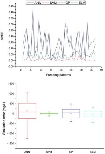
The AARE values obtained by the data-based models when used to simulate salt water concentration, along with box plots to check whether the models are able to capture the variations in the given dataset, are presented in Figures 2–6 for PW1–PW5, respectively, and Figures 7 and 8 for OW1 and OW2. The AARE results for the pumping and observation wells show that the salt water concentration obtained using the SVM model has the least error. The AARE for the ELM model is greater than that for the SVM, while it is much lower than that of the ANN and GP models. The box plots show the variability of model performance for the simulation of salt water intrusion for the ANN, SVM, GP and ELM models. The box plots for all pumping and observation wells suggest that the variation is best mapped by the SVM model. The ELM results are superior to those of the ANN and GP models, but inferior to those of the SVM. The simulation errors are very close to zero for both SVM and ELM models, which supports the effectiveness of the optimum model structure obtained.

Figure 2. Average absolute relative error (AARE) and box plot of ANN, SVM, GP and ELM in simulating the salt water concentration at PW1.

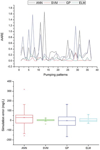
Figure 3. Average absolute relative error (AARE) and box plot of ANN, SVM, GP and ELM in simulating the salt water concentration at PW2.

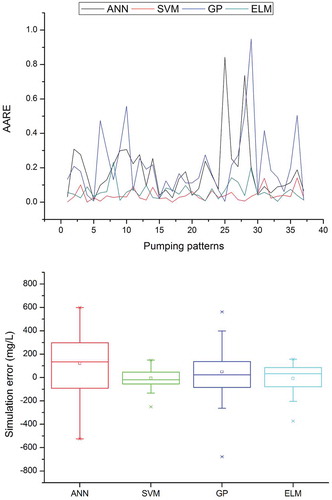
Figure 4. Average absolute relative error (AARE) and box plot of ANN, SVM, GP and ELM in simulating the salt water concentration at PW3.

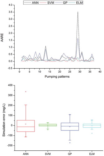
Figure 5. Average absolute relative error (AARE) and box plot of ANN, SVM, GP and ELM in simulating the salt water concentration at PW4.

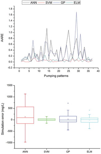
Figure 6. Average absolute relative error (AARE) and box plot of ANN, SVM, GP and ELM in simulating the salt water concentration at PW5.

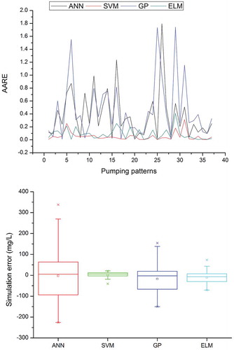
Figure 7. Average absolute relative error (AARE) and box plot of ANN, SVM, GP and ELM in simulating the salt water concentration at OBW1.

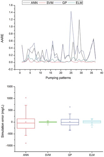
Figure 8. Average absolute relative error (AARE) and box plot of ANN, SVM, GP and ELM in simulating the salt water concentration at OBW2.

Overall, the results of the SVM and ELM models are superior to those of the ANN and GP models in the simulation of salt water intrusion. Comparing the results of the SVM and ELM models, both models have advantages and disadvantages. Convincingly, the error values (RMSE and AARE) of the SVM model are lower than those of the ELM model, while the NSE and R values of the ELM model for all locations are very close to those of the SVM model. In spite of the excellent simulation ability of the ELM model, the AARE is greater than that of the SVM model, which can be attributed to the fact that the training data had large variability and the model may not be sufficiently trained for such data. The major limitation of data-based models such as ELM is that it is a black-box model, which fails to simulate the internal physical processes of salt water intrusion. For the ELM model, being a data-driven technique, simulation ability could be increased by providing an appropriate and large number of input–output datasets for training. The model selection for the simulation of salt water intrusion should be a balanced approach based on the simulation accuracy as well as the level of complexities when designing the model architecture.

3.2 ANN, SVM and ELM as proxy simulators

The ANN, SVM, GP and ELM models were used in this study as proxy simulators for the three-dimensional, variable-density, coupled flow and solute-transport processes in coastal aquifers. The accuracy of the simulation was evaluated using statistical indicators and simulation plots (Figs 2–8), which clearly show that, of all the selected models, the SVM model yields the best results. However, it is important to note that the ELM model performs very close to the SVM in terms of simulation accuracy. Although the performance statics of the SVM and ELM are close in terms of accuracy, the main feature of ELM is its fast computational ability. Further analysis was thus conducted to determine the best data-based model amongst the models in terms of both accuracy and computational ability. A separate analysis was conducted to determine the CPU (central processing unit) time taken by each of the data-based models (ANN, SVM, GP and ELM) to simulate the given dataset. Table 4 presents the CPU time taken by the four proxy simulators to simulate a dataset of 287 × 6 (row × column), of which 250 × 6 sets are used for the training and the remainder used for testing. The performance of the SVM and ELM models is, respectively, six and 22 times faster than that of the ANN model. Although the SVM model is significantly faster than the ANN model, the ELM model takes a third of the time to compute the same dataset compared to the SVM model. The difference in time taken between the ANN and ELM models is substantial, but it is negligible between the GP and ELM models. Fast computational ability of proxy simulators becomes important when these simulators are used in combination with optimization techniques, since multiple recalling of simulators during optimization is time consuming. A notable fact about the ELM model is that the time taken for simulation also includes random selection of input weight and bias of hidden neurons, thus only hidden neurons need to be selected manually. In the case of the ANN, SVM and GP models, however, the simulation time does not include the time taken to tune the model parameters, which is otherwise extremely important to obtain accurate results but is time consuming. Thus, use of the ELM model as a proxy simulator saves a considerable amount of time during simulation and the model development also requires less time than when ANN, SVM and GP are chosen as proxy simulators.

Table 4. Comparison of the computational time taken by the ANN, SVM, GP and ELM models for the simulation of the dataset generated by SEAWAT.

Dataset size (row × column)	Model	CPU time (s)
Training: 250 × 6	ANN	11
Testing: 37 × 6
Training: 250 × 6	SVM	1.6
Testing: 37 × 6
Training: 250 × 6	GP	1.2
Testing: 37 × 6
Training: 250 × 6	ELM	0.5
Testing: 37 × 6

4 Conclusion

The numerical simulation of the salt water intrusion process in a coastal aquifer is complex and time-consuming as both flow and transport processes are highly nonlinear. Four data-based models (ANN, SVM, GP and ELM) were considered as proxy simulators to simulate the complex transient three-dimensional flow and transport processes in a coastal aquifer. The input dataset for the proxy simulators was generated by applying a finite-difference-based numerical simulation model, SEAWAT, to a typical confined aquifer. The performance of the developed models was evaluated and the results show that all proxy simulators are able to simulate the complex process of salt water intrusion with high accuracy. The newly tested data-based models, SVM and ELM, outperformed the ANN and GP models, yielding salt concentration values close to the SEAWAT model. The error analyses for the five pumping and two observation wells show that the SVM model is the most accurate; however, the computational time taken by the ELM model is considerably less than that of the SVM model. The generalization ability of the SVM model is superior to that of the ANN, GP and ELM models, as these models are more sensitive to the input structure and lead time than the SVM model. Unlike the process-based models, SVM and ELM do not require basin information and other physical parameters in the modelling process, which reduces the modelling complexities of the system. Thus, data-based model such as SVM and ELM can also be utilized for salt water intrusion modelling, considering that the training dataset should be large enough so that the model architectures can capture the involved complexities adequately.

Disclosure statement

No potential conflict of interest was reported by the authors.

References

- Abd-Elhamid, H.F. and Javadi, A.A., 2011. A cost-effective method to control seawater intrusion in coastal aquifers. Water Resources Management, 25 (11), 2755–2780. doi:10.1007/s11269-011-9837-7
- Acharya, N., et al., 2014. Development of an artificial neural network based multi-model ensemble to estimate the northeast monsoon rainfall over south peninsular India: an application of extreme learning machine. Climate Dynamics, 43 (5–6), 1303–1310. doi:10.1007/s00382-013-1942-2
- ASCE Task Committee on Application of Artificial Neural Networks in Hydrology, 2000. Artificial neural network in hydrology. I: preliminary concepts. Journal of Hydrologic Engineering, 5 (2), 115–123. doi:10.1061/(ASCE)1084-0699(2000)5:2(115)
- Ashtiani, A.B., Ketabchi, H., and Rajabi, M.M., 2013. Optimal management of a freshwater lens in a small island using surrogate models and evolutionary algorithms. Journal of Hydrologic Engineering, 19 (2), 339–354. doi:10.1061/(ASCE)HE.1943-5584.0000809
- Aytek, A. and Kişi, Ö., 2008. A genetic programming approach to suspended sediment modelling. Journal of Hydrology, 351 (3), 288–298. doi:10.1016/j.jhydrol.2007.12.005
- Banerjee, P., et al., 2011. Artificial neural network model as a potential alternative for groundwater salinity forecasting. Journal of Hydrology, 398 (3), 212–220. doi:10.1016/j.jhydrol.2010.12.016
- Bear, J., et al., 1999. Seawater intrusion in coastal aquifers – concepts, methods and practices. Dordrecht, Netherlands: Kluwer Academic.
- Bhattacharjya, R.K. and Datta, B., 2009. ANN-GA-based model for multiple objective management of coastal aquifers. Journal of Water Resources Planning and Management, 135 (5), 314–322. doi:10.1061/(ASCE)0733-9496(2009)135:5(314)
- Bhattacharjya, R.K., Datta, B., and Satish, M.G., 2007. Artificial neural networks approximation of density dependent saltwater intrusion process in coastal aquifers. Journal of Hydrologic Engineering, ASCE, 12 (3), 273–282. doi:10.1061/(ASCE)1084-0699(2007)12:3(273)
- Chekirbane, A., et al., 2015. 3D simulation of a multi-stressed coastal aquifer, northeast of Tunisia: salt transport processes and remediation scenarios. Environmental Earth Sciences, 73 (4), 1427–1442. doi:10.1007/s12665-014-3495-z
- Choy, K. and Chan, C., 2003. Modelling of river discharges and rainfall using radial basis function networks based on support vector regression. International Journal of System Science, 34 (1), 763–773. doi:10.1080/00207720310001640241
- Cobaner, M., et al., 2012. Three dimensional simulation of seawater intrusion in coastal aquifers: A case study in the Goksu Deltaic Plain. Journal of Hydrology, 464, 262–280. doi:10.1016/j.jhydrol.2012.07.022
- Deka, P.C., 2014. Support vector machine applications in the field of hydrology: a review. Applied Soft Computing, 19, 372–386. doi:10.1016/j.asoc.2014.02.002
- Dhar, A. and Datta, B., 2009. Saltwater intrusion management of coastal aquifers. I: linked simulation-optimization. Journal of Hydrologic Engineering, 14 (12), 1263–1272. doi:10.1061/(ASCE)HE.1943-5584.0000097
- Ferreira, C., 2006. Gene expression programming: mathematical modeling by an artificial intelligence. Berlin, Germany: Springer-Verlag.
- Francone, F., 2000. DiscipulusTM owner’s manual, version 3.0. Register machine learning technologies.
- Gizaw, M.S. and Gan, T.Y., 2016. Regional flood frequency analysis using support vector regression under historical and future climate. Journal of Hydrology, 538, 387–398. doi:10.1016/j.jhydrol.2016.04.041
- Gopinath, S., et al., 2016. Modeling saline water intrusion in Nagapattinam coastal aquifers, Tamilnadu, India. Modeling Earth Systems and Environment, 2 (1), 1–10. doi:10.1007/s40808-015-0058-6
- Guo, W. and Langevin, C.D., 2002. User’s guide to SEAWAT: A computer program for the simulation of three-dimensional variable-density ground-water flow [online]. US geological survey techniques of water resources investigations, Book 6, Chapter A7. Available from: http://pubs.er.usgs.gov/publication/twri06A7.
- Harbaugh, A.W., Banta, E.R., Hill, M.C., and McDonald, M.G., 2000. MODFLOW-2000, the US Geological survey modular groundwater model – user guide to modularization concepts and the groundwater flow process. US Geological Survey, Open-File Report 00-92.
- Harpham, C. and Dawson, C.W., 2006. The effect of different basis functions on a radial basis function network for time series prediction: a comparative study. Neurocomputing, 69 (16–18), 2161–2170. doi:10.1016/j.neucom.2005.07.010
- Holding, S. and Allen, D.M., 2016. Risk to water security for small islands: an assessment framework and application. Regional Environmental Change, 16 (3), 827–839. doi:10.1007/s10113-015-0794-1
- Holzbecher, E., 1998. Modeling density-driven flow in porous media: principles, numerics, software. Berlin, Germany: Springer-Verlag.
- Huang, G.B., Zhu, Q.Y., and Siew, C.K., 2004. Extreme learning machine: a new learning scheme of feedforward neural networks. Proceedings of 2004 IEEE the international joint conference on neural networks, 25–29 July 2004 Hungary. Budapest: IEEE. Vol. 2, 985–990.
- Huang, G.B., Zhu, Q.Y., and Siew, C.K., 2006. Extreme learning machine: theory and applications. Neurocomputing, 70, 489–501. doi:10.1016/j.neucom.2005.12.126
- Hussain, M.S., et al., 2015. A surrogate model for simulation–optimization of aquifer systems subjected to seawater intrusion. Journal of Hydrology, 523, 542–554. doi:10.1016/j.jhydrol.2015.01.079
- Juster, T.C., 1995. Circulation of saline and hypersaline groundwater in carbonate mud: mechanisms, rates, and an example from Florida Bay. Dissertation (PhD). Department of Geology, University of South Florida-Tampa, USA.
- Kourakos, G. and Mantoglou, A., 2009. Pumping optimization of coastal aquifers based on evolutionary algorithms and surrogate modular neural network models. Advances in Water Resources, 32 (4), 507–521. doi:10.1016/j.advwatres.2009.01.001
- Kourakos, G. and Mantoglou, A., 2013. Development of a multi-objective optimization algorithm using surrogate models for coastal aquifer management. Journal of Hydrology, 479, 13–23. doi:10.1016/j.jhydrol.2012.10.050
- Langevin, C.D., Swain, E.D., and Wolfert, M.A., 2005. Simulation of integrated surfacewater/ground-water flow and salinity for a coastal wetland and adjacent estuary. Journal of Hydrology, 314, 212–234. doi:10.1016/j.jhydrol.2005.04.015
- Lecca, G., 2000. Implementation and testing of the CODESA-3D model for density-dependent flow and transport problems in porous media. Pula, Italy: Environment Area, CRS4.
- Liang, N.Y., et al., 2006. A fast and accurate online sequential learning algorithm for feedforward networks. Neural Networks, IEEE Transactions, 17 (6), 1411–1423. doi:10.1109/TNN.2006.880583
- Lin, H.J., et al., 1997. A three-dimensional finite-element computer model for simulating density-dependent flow and transport in variable saturated media: version 3.1. Vicksburg, MS: US Army Engineering Research and Development Center.
- Lin, J., et al., 2009. A modeling study of seawater intrusion in Alabama Gulf Coast, USA. Environmental Geology, 57, 119–130. doi:10.1007/s00254-008-1288-y
- Lin, J.Y., Cheng, C.T., and Chau, K.W., 2006. Using support vector machines for long-term discharge prediction. Hydrological Sciences Journal, 51 (4), 599–612. doi:10.1623/hysj.51.4.599
- Mohammadi, K., et al., 2015. Extreme learning machine based prediction of daily dew point temperature. Computers and Electronics in Agriculture, 117, 214–225. doi:10.1016/j.compag.2015.08.008
- Morgan, L.K., Werner, A. D., Morris, M. J., and Teubner, M. D., 2013. Application of a rapid-assessment method for seawater intrusion vulnerability: Willunga Basin, South Australia. Groundwater in the coastal zones of Asia-Pacific. Dordrecht: Springer Netherlands, 205–225.
- Nash, J.E. and Sutcliffe, J.V., 1970. River flow forecasting through conceptual models part I – A discussion of principles. Journal of Hydrology, 10 (3), 282–290. doi:10.1016/0022-1694(70)90255-6
- Nikam, V. and Gupta, K., 2013. SVM-based model for short-term rainfall forecasts at a local scale in the Mumbai urban area, India. Journal of Hydrologic Engineering, 19 (5), 1048–1052. doi:10.1061/(ASCE)HE.1943-5584.0000875
- Oude Essink, G.H.P., 1998. MOC3D adapted to simulate 3D density-dependent groundwater flow. In: Proceedings of MODFLOW ’98 conference at the international ground water modeling center. Golden, Colorado: Colorado School of Mines, Vol. 1, 291–300.
- Qahman, K. and Larabi, A., 2006. Evaluation and numerical modeling of seawater intrusion in the Gaza aquifer (Palestine). Hydrogeology Journal, 14 (5), 713–728. doi:10.1007/s10040-005-003-2
- Qu, J. and Zuo, M.J., 2010. Support vector machine based data processing algorithm for wear degree classification of slurry pump systems. Measurement, 43 (6), 781–791. doi:10.1016/j.measurement.2010.02.014
- Rao, S.V.N., et al., 2004. Planning groundwater development in coastal aquifers. Hydrological Sciences Journal, 49 (1), 155–170. doi:10.1623/hysj.49.1.155.53999
- Roy, D.K. and Datta, B., 2017. Fuzzy C-mean clustering based inference system for saltwater intrusion processes prediction in coastal aquifers. Water Resources Management, 31 (1), 355–376. doi:10.1007/s11269-016-1531-3
- Sanford, W.E. and Konikow, L.F., 1985. A two-constituent solute transport model for ground water having variable density. In: US geological survey water-resources investigations report 85–4279.
- Schalkoff, R.J., 1997. Artificial neural networks. New York, NY: Wiley.
- Schmid, M.D., 2009. A neural network package for Octave user’s guide version: 0.1. 9.1. (plexso.com).
- Schneider, J.C. and Kruse, S.E., 2006. Assessing selected natural and anthropogenic impacts on freshwater lens morphology on small barrier Islands: dog Island and St. George Island, Florida, USA. Hydrogeology Journal, 14, 131–145. doi:10.1007/s10040-005-0442-9
- Shamshirband, S., et al., 2015a. Application of extreme learning machine for estimation of wind speed distribution. Climate Dynamics, 46 (5–6), 1893–1907. doi:10.1007/s00382-015-2682-2
- Shamshirband, S., et al., 2015b. A comparative evaluation for identifying the suitability of extreme learning machine to predict horizontal global solar radiation. Renewable and Sustainable Energy Reviews, 52, 1031–1042. doi:10.1016/j.rser.2015.07.173
- Sreekanth, J. and Datta, B., 2010. Multi-objective management of saltwater intrusion in coastal aquifers using genetic programming and modular neural network based surrogate models. Journal of Hydrology, 393 (3–4), 245–256. doi:10.1016/j.jhydrol.2010.08.023
- Sreekanth, J. and Datta, B., 2011. Coupled simulation-optimization model for coastal aquifer management using genetic programming-based ensemble surrogate models and multiple-realization optimization. Water Resources Research, 47, W04516. doi:10.1029/2010WR009683
- Sreekanth, J. and Datta, B., 2014. Stochastic and robust multi-objective optimal management of pumping from coastal aquifers under parameter uncertainty. Water Resources Management, 28 (7), 2005–2019. doi:10.1007/s11269-014-0591-5
- Suryanarayana, C., et al., 2014. An integrated wavelet-support vector machine for groundwater level prediction in Visakhapatnam, India. Neurocomputing, 145, 324–335. doi:10.1016/j.neucom.2014.05.026
- Taormina, R. and Chau, K.W., 2015. Data-driven input variable selection for rainfall–runoff modeling using binary-coded particle swarm optimization and extreme learning machines. Journal of Hydrology, 529, 1617–1632. doi:10.1016/j.jhydrol.2015.08.022
- Vapnik, V., 1995. The nature of statistical learning theory. New York, NY: Springer-Verlag.
- Vapnik, V., 2000. The nature of statistical learning theory. 2nd ed. New York, NY: Springer-Verlag.
- Vapnik, V.N. and Vapnik, V., 1998. Statistical learning theory. New York, NY: Wiley, Vol. 1.
- Vijay, R. and Mohapatra, P.K., 2016. Hydrodynamic assessment of coastal aquifer against saltwater intrusion for city water supply of Puri, India. Environmental Earth Sciences, 75 (7), 1–8. doi:10.1007/s12665-016-5357-3
- Voss, C.I., 1984. A finite-element simulation model for saturated–unsaturated, fluid-density-dependent ground-water flow with energy transport or chemically reactive single-species solute transport. Reston, VA: US Geological Survey, US Geological Survey Water-Resources Investigations Report 84-4369.
- Wang, W.C., et al., 2009. A comparison of performance of several artificial intelligence methods for forecasting monthly discharge time series. Journal of Hydrology, 374 (3), 294–306. doi:10.1016/j.jhydrol.2009.06.019
- Wang, W.C., et al., 2013. Improved annual rainfall–runoff forecasting using PSO–SVM model based on EEMD. Journal of Hydroinformatics, 15 (4), 1377–1390. doi:10.2166/hydro.2013.134
- Wang, X. and Han, M., 2014. Online sequential extreme learning machine with kernels for non-stationary time series prediction. Neurocomputing, 145, 90–97. doi:10.1016/j.neucom.2014.05.068
- Yadav, B., et al., 2016a. Discharge forecasting using an Online Sequential Extreme Learning Machine (OS-ELM) model: a case study in Neckar River, Germany. Measurement, 92, 433–445. doi:10.1016/j.measurement.2016.06.042
- Yadav, B., et al., 2016b. Estimation of in-situ bioremediation system cost using a hybrid Extreme Learning Machine (ELM)-particle swarm optimization approach. Journal of Hydrology, 543, 373–385. doi:10.1016/j.jhydrol.2016.10.013
- Yang, J., et al., 2009. Group-sensitive multiple kernel learning for object categorization. In: 2009 IEEE 12th international conference on computer vision. IEEE, 436–443.
- Yu, P.S., Chen, S.T., and Chang, I.F., 2006. Support vector regression for real-time flood stage forecasting. Journal of Hydrology, 328 (3), 704–716. doi:10.1016/j.jhydrol.2006.01.021
- Yu, X., Liong, S., and Babovic, V., 2004. EC-SVM approach for real-time hydrologic forecasting. Journal of Hydroinformatics, 6 (3), 209–223.
- Zhao, Z., Li, P., and Xu, X., 2013. Forecasting model of coal mine water inrush based on extreme learning machine. Applied Mathematics & Information Sciences, 7, 1243–1250. doi:10.12785/amis/070349