Effect of input data in hydraulic modeling for flood warning systems

ABSTRACT

The main objective of this study was to quantify the error associated with input data, including various resolutions of elevation datasets and Manning’s roughness for travel time computation and floodplain mapping. This was accomplished on the test bed, the Grand River (Ohio, USA) using the HEC-RAS model. LiDAR data integrated with survey data provided conservative predictions, whereas coarser elevation datasets provided a positive difference in the travel time (11.03–15.01%) and inundation area (32.56–44.52%). The minimum differences in travel time and inundation area were 0.50–4.33% and 3.55–7.16%, respectively, when the result from LiDAR integrated with survey data was compared with a 10-m DEM integrated with survey data. The results suggest that a 10-m DEM in the channel and LiDAR data in the floodplain combined with survey data would be appropriate for a flood warning system. Additionally, Manning’s roughness of the channel section was found to be more sensitive than that of the floodplain. The decrease in inundation area was highest (8.97%) for the lower value of Manning’s roughness.

KEYWORDS:

• floodplain mapping
• topographic dataset
• river bathymetry
• HEC-RAS
• HEC-GeoRAS

EDITOR A. Castellarin; ASSOCIATE EDITOR G. Di Baldassarre

1 Introduction

Flooding is one of the most common natural hazards in many countries across the world; it causes millions of dollars of damage to property and may take the lives of thousands of people every year (Lowe 2003, Basha and Daniela 2007, King 2009). The NatCat service of Munich Re (2011) provides a list of the 10 costliest floods from 1980 to 2011, with a cumulative loss of about US$200 billion. Floods have caused more human deaths and property losses (90% of all property losses) than any other form of natural hazard in the 20th century in the United States (Krimm 1996, Perry 2000). One of the ways to minimize the losses from such hazards is to develop a flood warning system and inform the people in the community for evacuation with sufficient lead time. Therefore, the determination and communication of flood travel (evacuation) time is essential for the timely evacuation of people from probable inundation areas and to minimize the adverse consequences of such hazards (Krzysztofowicz et al. 1994). However, it is equally important to make such floodplain maps easily accessible and comprehensible to the public (Holtzclaw et al. 2005). Floodplain maps are very important tools that represent the spatial variability of flood hazards and provide more direct and robust understanding of floods than any other forms (Merz et al. 2007, Leedal et al. 2010). While there has been significant advancement in hydrological and hydraulic models to generate floodplain maps, uncertainties associated with topography, flow discharge and modeling approach still exist in the floodplain mapping process (Marks and Bates 2000, Crosetto and Tarantola 2001, Smemoe et al. 2012, Merwade et al. 2008, Bales and Wagner 2009). Since the floodplain mapping process is not an exact science (Smemoe et al. 2012), probabilistic floodplain maps generated considering uncertainties in modeling are more appropriate than deterministic maps when planning for the future rescue operations and quantification of flood insurance rates in probable affected areas (Di Baldassarre 2012).

Various studies have been conducted to study the uncertainties associated with the flood inundation mapping process. Merwade et al. (2008) conducted a study of floodplain mapping in Strouds Creek, North Carolina, USA, and reported the uncertainties due to hydrological flow, including the complex interaction of individual inputs in the hydraulic model. Similarly, another study was conducted in Strouds Creek and Brazos River in Texas (Cook and Merwade 2009) to study the effects of topographic data and the geometric configuration on flood inundation maps. These studies concluded that the predicted area decreases with higher resolution of topographic data. Similarly, other studies (Horritt and Bates 2001, Bates et al. 2004, Domeneghetti et al. 2013, Dottori et al. 2013) have been conducted to comprehend the uncertainties in flood inundation maps. However, to the best of our knowledge, quantification of the potential uncertainties in flood travel time of various return periods for different elevation datasets and Manning’s roughness values have not been studied significantly. The motivation of this research was to explore the implications of input data for evacuation time and flood area prediction for the possible improvement of flood warning systems. Therefore, the major objective of this research was to calculate the flood travel time and then generate floodplain maps corresponding to different return period floods in the City of Painesville, located along the Grand River of Lake County, Ohio. The travel time was computed using predicted steady flow velocity and longitudinal distance of river sections. The steady flow approach was used, which is reasonable for high flows, although the travel time is somewhat nonlinear at low flows (Pilgrim 1976). The uncertainties associated with flood travel time and the extent of flood inundation maps when using various resolutions of elevation datasets and different values of Manning’s roughness are also reported. Hence, the HEC-RAS model was developed for flood magnitudes of different return periods. Finally, the effects of elevation data resolution and Manning’s roughness are reported for the appropriate representation of flood travel time and flood extents.

2 Theoretical description

The hydraulic modeling software, HEC-RAS, was used in this study for steady and unsteady flow analysis. The HEC-RAS model was developed by the US Army Corps of Engineers – Hydrologic Engineering Center (USACE-HEC), and has been widely used for steady flow analysis, unsteady flow simulation, movable boundary sediment transport computations and water quality analysis (Brunner 1995). Usually, the steady flow approach is used for floodplain management and flood insurance studies (Cook and Merwade 2009), whereas the unsteady flow approach is used especially for dam break analysis and pressurized flow modules (Brunner 1995, 2002). The effects of various obstructions such as culverts, bridges, dams and weirs can be considered in the analysis to see their impacts in the water surface profiles. The HEC-RAS model solves one-dimensional Saint Venant equations, using a four-point implicit method developed for natural channels (Brunner 2002) to simulate unsteady flow, which is derived from the continuity and momentum equations. The continuity and momentum equations are as follows:

(1)

(2)

where Q is discharge of the river; A is cross-sectional area normal to the flow; t is any time; x is longitudinal distance in the river; g is acceleration due to gravity; H is elevation of water surface in the river above an assumed datum level; S₀ is slope of the river bed, and S_f is energy slope of water.

The Saint Venant equations are solved using the four-point implicit finite difference scheme. This scheme is completely non-destructive but marginally stable (Fread 1974, Liggett and Jean 1975) when it is run in semi-implicit form (corresponds to a weighting factor θ of 0.5).

In steady flow simulation, HEC-RAS solves the energy equation (Equation (3)) to calculate water surface profiles from one cross-section to another with an iterative procedure called the standard step method (Brunner 1995):

(3)

where Z₁ and Z₂ are elevations of the main channel; Y₁ and Y₂ are depths of water; V₁ and V₂ are average velocities; a₁ and a₂ are velocity weighting coefficients at sections one and two, respectively; g is acceleration due to gravity; and H_e is energy head loss from section one to section two.

3 Materials and methodology

3.1 Study area

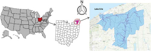
This study was conducted in the Grand River watershed, which consists of major three tributaries: the Mill, Paine and Big Creeks. The watershed is located in northeastern Ohio and has an area of 705 square miles (1826 km²), with an elevation range from a minimum of 564 feet (172 m) to a maximum of 1385 feet (422 m) a.m.s.l. (Fig. 1). It has 28 HUC-14 (Hydrologic Unit Code) watersheds and six HUC-11 watersheds, which cover five counties: Lake, Ashtabula, Trumbull, Geauga and Portage. The watershed is geographically within 41°22′–41°51′N and 80°35′–81°18′E. The Grand River originates from the southern part of Middlefield and flows through Orwell, Rock Creek, Austinburg, Harpersfield, Madison, Perry, Painesville and Fairport Harbor, and finally discharges into Lake Erie. The river is approximately 102.7 miles (165 km) long, with an average slope of 1:900 and an average width of approximately 84 feet, varying from 150 to 500 feet (46–152 m) in width at various locations. The mean annual precipitation in the watershed is 38 inches (96.5 cm) based on historical records. In this study, a river section of approximately 32.2 miles (52 km) between Harpersfield and Fairport Harbor, which includes the City of Painesville, was considered as a study site to perform the hydraulic analysis.

Figure 1. Study area of the Grand River, Ohio, USA (Grand River watershed).

The City of Painesville along the Grand River experienced flooding in 2006, 2008 and 2011. The disastrous flood of 27–28 July 2006 on the Grand River was caused by more than 11 inches (28 cm) of rainfall, and overtopped the embankments, leading to the destruction of 100 homes and businesses, five bridges and 13 roads. Property worth US$30 million was damaged and there was one death in Lake County. Consequently, hundreds of people were evacuated and three counties (Lake, Geauga and Ashtabula) were declared Federal and State disaster areas (Ebner et al. 2006). This flood was reported to have a peak flow of 35 000 cfs (991 m³/s) (500-year return period) and the highest historic stage of 19.35 feet (5.9 m) (Ebner et al. 2006) as recorded by USGS gage station 04212100 near the City of Painesville.

3.2 Overall modeling approach

To calculate accurate flood travel time and generate floodplain maps, the calibrated and validated one-dimensional hydraulic model, HEC-RAS, was developed by importing the geospatial data of river cross-sections and bridges from HEC-GeoRAS. The HEC-GeoRAS is a tool for processing geospatial data in ArcGIS using a graphical user interface. One-dimensional (1D) unsteady flow simulation for different flood events for the period 1996–1998 was performed for model calibration and validation. The 1D method of hydraulic modeling is considered to be computationally efficient to calculate the floodplain and flood extents, especially for higher flows, regardless of limited topographical datasets (Horritt and Bates 2001). However, the 1D model may have some limitations in overestimating or underestimating the floodplain extents, as volume information is not included in the floodplain delineation, leading to the importance of modern 2D modeling methods (Bates and De Roo 2000, Cook and Merwade 2009, Jung et al. 2011). There have been mixed responses regarding the use of 1D and 2D models. For example, some studies suggest that simulation through 1D and 2D models is not significantly different (Horritt and Bates 2002), whereas Cook and Merwade (2009) reported that the 1D model slightly underpredicts the inundation area. However, Alho and Aaltonen (2008) reported that 1D modeling provided comparable results to data derived from 2D simulation. Similarly, Costabile et al. (2015) reported that using LiDAR data can provide detailed topographic information, which can significantly improve the 1D computations. Also, they reported that the 1D model can be used with greater hydraulic skillfulness. Tayefi et al. (2007) reported that a coupled 1D–2D treatment could be the best modeling approach.

Nevertheless, 1D steady flow simulation is still typically performed during peak flood periods (Hicks and Peacock 2005, Cook 2008, Whitehead and Ostheimer 2009, Ostheimer 2012) to calculate the flood extents. Peak flood was simulated in steady flow conditions to calculate the flood travel time and water surface elevations. Two-dimensional unsteady flow simulation was also performed to compare the results obtained from 1D unsteady flow simulation. As mentioned earlier, the travel time was computed using predicted steady flow velocity and longitudinal distance of river sections. These calculated water surface elevations/extents were then exported back to HEC-GeoRAS to produce floodplain maps. Typically, elevation datasets such as National Elevation Datasets (NED) and LiDAR do not include the river bathymetry, leading to the requirement of field verification through a topographical survey. Therefore, the river was surveyed using a highly accurate Global Positioning System (GPS) Rover, which uses the state Virtual Reference Station (VRS) System and allows real time kinematic (RTK) positioning using a single rover in the field, with no need to set up a base station. The survey was conducted from Harpersfield to North St. Clair Bridge. For the remaining portion, up to Lake Erie near Fairport Harbor, a bathymetry survey using the sounding method produced by the National Oceanic and Atmospheric Administration (NOAA) and USACE was used. Six different topographical datasets were used in this study: LiDAR-derived DEM, 10-m DEM, 30-m DEM, and integration of field-verified cross-sections with each dataset of LiDAR-derived DEM, 10-m DEM and 30-m DEM. The integration of field-verified cross-sections with LiDAR-derived DEM, 10-m DEM and 30-m DEM was performed in a similar way as described in Merwade et al. (2008). The sources for the various DEMs are presented in Table 1. The differences in travel time and floodplain extent were compared and reported using the different datasets.

Table 1. Datasets used in the study.

Type of data	Data	Source
GIS	LiDAR derived DEM	OGRIP http://gis3.oit.ohio.gov/geodatadownload/osip.aspx
	National Land Cover Datasets 2011	United States Department of Agriculture, Natural Resources Conservation Service (USDA, NRCS) Geospatial Data Gateway https://gdg.sc.egov.usda.gov/
	Digital georeferenced aerial photography	Ohio Statewide Imagery Program (Ohio Department of Administrative Services 2007) http://ogrip.oit.ohio.gov/
	DEMs 10-m, 30-m	USDA, NRCS Geospatial Data Gateway https://gdg.sc.egov.usda.gov/
Hydrology	Streamflow (discharge) and water surface stage	United States Geological Survey (USGS) http://waterdata.usgs.gov/usa/nwis/uv?04212100 http://waterdata.usgs.gov/usa/nwis/sw
Climate	Precipitation and temperature	NOAA/National Climatic Data Center (NCDC) http://www.ncdc.noaa.gov/cdo-web/
Bridge data	Engineering drawing of bridges	Lake County Office http://www.lakecountyohio.gov/ Ohio Department of Transportation http://www.dot.state.oh.us/

3.3 HEC-GeoRAS/HEC-RAS model input

Elevation datasets are needed to generate geospatial data and perform hydraulic analysis in HEC-RAS. Therefore, high-quality datasets were used in this study in order to compute travel times and produce better flood inundation maps. LiDAR data were downloaded from the Ohio Geographically Referenced Information Program (OGRIP) website. Similarly, DEMs of 10- and 30-m resolution were downloaded from the National Resource Conservation Service – US Department of Agriculture (NRCS-USDA), Geospatial Data Gateway. The elevation data for the Grand River from those DEMs were extracted using HEC-GeoRAS, an extension of ArcGIS. Typically, LiDAR data are more accurate compared to 10-m and 30-m DEM. Sanders (2007) reported the vertical accuracy of LiDAR as ±0.2–0.25 m, that of 10-m DEM as ±7 m and of 30-m DEM as ±7–15 m. However, this range of error was reported based on a study conducted throughout the continental United States and the higher discrepancy is typically near waterbodies. For the study area, the error level was not significant even for the 30-m DEM based on the comparison of cross-sections generated by 30-m DEM with field-verified cross-sections.

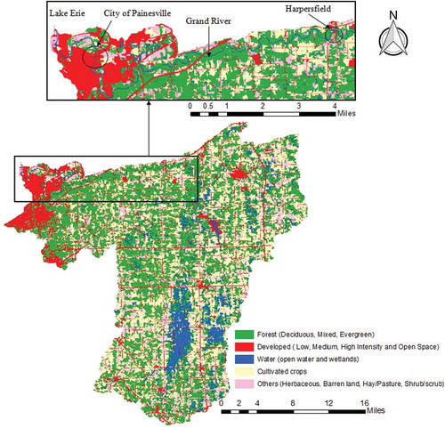
Land-use data at 30-m resolution were downloaded from National Land Cover Database 2011 (NLCD 2011). The Grand River watershed includes forest (41.86%), cultivated land (24.57%), waterbodies and wetlands (7.67%) and developed/urban land (10.21%). The remaining 15.70% is covered by other land, such as herbaceous (4.2%), barren land (0.08%), hay/pasture (9.29%) and shrub/scrub (2.13%) as per NLCD 2011 (Fig. 2).

Figure 2. Land-use data (30-m resolution) map of the Grand River watershed, Ohio. NLCD (2011).

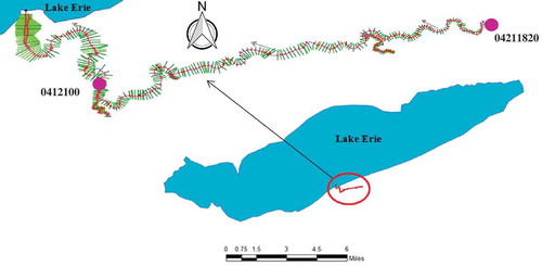
Geometric input feature classes needed for HEC-RAS, such as stream lines, cross-sections, bank stations and storage areas, were first created in HEC-GeoRAS and then exported to HEC-RAS. In order to represent the river cross-section accurately in the model, the topographical survey was performed at 77 different sections of the river (Fig. 3) and the cross-sections between surveyed cross-sections were interpolated. The cross-sections were surveyed at intervals of half a mile to a mile depending upon the site conditions. Readers can find a detail discussion about the selection of cross-section locations in various journal articles (Samuels 1990, Castellarin et al. 2009). The hydraulic model, HEC-RAS, developed for the Grand River after incorporating river cross-sections is shown in Figure 4. Discharge and stage data for stations 04211820 (upstream gage station near Harpersfield) and 04212100 (downstream gage station near the City of Painesville) were obtained from the USGS website to perform unsteady hydraulic analysis and calibrate Manning’s roughness for study reaches in HEC-RAS. Peak discharge data for the recurrence intervals of 10, 50, 100 and 500 years for the Grand River were obtained from Koltun and Roberts (1990), which were determined based on log-Pearson Type III distribution. For other ungauged stream reaches including Mill, Paine and Big Creek, peak discharges from 10- to 500-year return periods were obtained from the streamstat web application (Guthrie et al. 2008). The streamstat calculates the peak discharge based on different regression equations (Koltun and Roberts 1990) depending upon the river basin characteristics. There are 10 bridges within the study area, and the data for these bridges were obtained from Lake County Office and Ohio Department of Transportation (ODOT). Similarly, the data for high flood levels for Lake Erie have been obtained from a report by USACE (USACE (US Army Corps of Engineers) 2000). A summary of input data including their types and sources is presented in Table 1.

Figure 3. LiDAR DEM with cross-section configurations of the Grand River. Red dots show where cross-sections from different elevation datasets are compared (as shown in Fig. 7); green dots show surveyed sections along the Grand River.

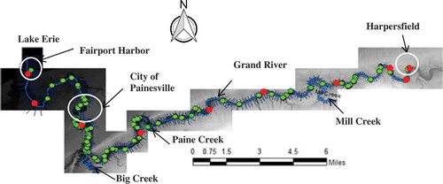
Figure 4. Hydraulic model of the Grand River as developed in HEC-RAS.

3.4 Model calibration and validation

The unsteady HEC-RAS model was calibrated by an iterative process to obtain a suitable value of Manning’s roughness for river reaches by comparing simulated stage and discharge with the observed data. The preliminary selection criterion of Manning’s roughness was recommended by various approaches including visual inspection, land use/land cover and optimization techniques rather than selecting it just intuitively (Kalyanapu et al. 2009). Channel roughness is highly variable as it depends on many factors such as channel alignment, surface roughness, bed material, nature of sediments and obstruction present in the channel (Pappenberger et al. 2005, Timbadiya et al. 2011, Parhi et al. 2012). Chow et al. (1988) illustrated that Manning’s roughness varies from 0.035 to 0.065 for the main channel and 0.08 to 0.15 in the floodplains. Regardless, it needs to be calibrated using the known years’ flood data; therefore, eight different flood events from 1996 to 1998 were used in HEC-RAS simulation. Finally, the calibrated Manning’s roughness values were used to calculate travel time and develop the flood inundation maps.

3.5 Model evaluation criteria

Various statistical parameters, namely Nash-Sutcliffe efficiency (NSE), correlation coefficient (R²), percent bias (PBIAS), root mean square error (RMSE) and ratio of RMSE and standard deviation (RSR), were used to test the accuracy and predictive power of the model (ASCE 1993, Gupta et al. 1999, Moriasi et al. 2007).

The NSE is a normalized statistic that determines the relative magnitude of the residual variance (“noise”) compared to the measured data variance (Nash and Sutcliffe 1970). The NSE is recommended for model evaluation as it has been found to be the best objective function for reflecting the overall fit of a hydrograph (Moriasi et al. 2007). Typically, it indicates the wellness of observed and simulated data fitting the 1:1 line. Its value ranges from −∞ to 1, and values from 0 to 1 are acceptable. An NSE value of 1 is rare and considered to be the perfect value for an ideal model. NSE is calculated by:

(4)

where is the ith value of observed data, is the ith value of simulated data, is the mean value of observed data, and n is the total number of observations.

The correlation coefficient, R², measures the fitness of observed and simulated data; R² varies from 0 to 1, indicating 1 as the perfect fitness of data, and is calculated by:

(5)

where is the mean of simulated data.

The RSR is the ratio of RMSE and standard deviation of the observed data. The lower the value of RSR, the lower is the RMSE and the better is the model performance. The ideal value of RSR is 0. The RSR is calculated by:

(6)

where SD is the standard deviation.

The percentage deviation in simulated data from the observed data (PBIAS) (Moriasi et al. 2007) with value 0 is considered as the perfect model harmonizing with the observed data. Negative values of PBIAS specify overestimation bias, whereas positive values of PBIAS indicate underestimation bias. PBIAS is calculated by:

(7)

4 Uncertainties associated with floodplain modeling

A large number of uncertainties accompanying numerous variables including topography, Manning’s roughness, flow and modeling technique are still associated with floodplain mapping, regardless of the advancements in hydrological and hydraulic modeling tools (Oegema and McBean 1987, Smemoe et al. 2012, Merwade et al. 2008). Therefore, the accuracy of the floodplain maps depends on how these uncertain variables have been incorporated in hydraulic and hydrological models (Merwade et al. 2008). Two important variables (topography and Manning’s roughness), which may impose errors in flood travel time and inundation area, are discussed in this study.

4.1 Effect of topography

Reliable elevation datasets are essential for the generation of accurate flood inundation maps. The use of high-resolution LiDAR data might somewhat improve the accuracy of floodplain mapping as it provides highly accurate elevation data. However, it does not represent the exact river bathymetry, which may still pose serious errors in travel time calculation and flood inundation mapping. According to Merwade et al. (2008), the poor quality of terrain data can impose errors in the flood inundation mapping process in three ways. First, it affects the discharge values estimated from hydrological models. Second, it affects water surface elevation calculated from hydraulic models, and finally, it affects the horizontal extent of floods. More importantly, errors in channel topography impact upon channel conveyance and connectivity of flow pathways. So, the field-verified cross-sections of river reaches are absolutely essential to get the better bathymetry of the river needed for travel time computation and floodplain mapping.

4.2 Effect of Manning’s roughness

Since the complete characteristics of a terrain are reflected in the effective roughness value, it plays a significant role in model calibration and floodplain delineation. The roughness value varies spatially along the river depending upon the river bed material and surrounding floodplain characteristics. It is essential to adequately represent the roughness characteristics of the floodplain and channel in order to reduce the uncertainties involved in the flood travel time and floodplain mappings. The preliminary selection of Manning’s roughness in the Grand River was based on terrain properties of other similar rivers. as presented in Arcement and Verne (1989) and Barnes (1849). The hydraulic model in this study was simulated for different values of channel roughness to study the uncertainties associated with it.

4.3 Effect of discharge

River discharge is also considered as one of the uncertain variables that has to be considered in floodplain mapping (Oegema and McBean 1987, Pappenberger et al. 2006, Merwade et al. 2008, Di Baldassarre and Montanari 2009) even though uncertainty in river discharge is typically related to the discharge that arises at a particular return period or flood event. The discharge values for various return period floods were generated from the regression equation derived by USGS (Koltun and Roberts 1990). Errors associated with discharge prediction for tributaries can be dissipated in water surface elevation and the flood extents calculated from the hydraulic model (Merwade et al. 2008).

5 Results and discussion

5.1 Simulation of hydraulic model

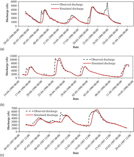
The performance of the model was good in calibration and validation based on an evaluation measured through different statistical criteria. The calculated values of all statistical parameters were higher than the recommended values (NSE > 0.50, PBIAS ±25% and RSR ≤ 0.70) of Moriasi et al. (2007). The detailed results of calibration/validation for the stage at upstream gage station 04211820 are presented in Table 2. Similarly, the detailed results of calibration/validation for discharge at downstream gage station 04212100 are presented in Table 3. In this study, NSE for stage calibration/validation varied from 0.74 to 0.89 (Table 3), and NSE for discharge calibration/validation varied from 0.69 to 0.96 (Table 3), except for the period 26 February to 3 March 1997. The model performance was tested with RMSE, which tends to be high for significantly higher flows.

Table 2. Calibration/validation for stage at upstream gage station 04211820.

	Date range		Statistical parameter
	From	To	NSE	R^2	PBIAS	RSR	RMSE (cfs)
Calibration
1	3/1/1996 0:00	3/30/1996 00:00	0.74	1.00	0.05	0.51	0.53
2	4/15/1996 0:00	5/12/1996 23:00	0.84	1.00	0.00	0.39	0.60
3	10/20/1996 0:00	11/28/1996 23:00	0.84	1.00	0.03	0.40	0.58
4	2/4/1997 0:00	2/10/1997 23:30	0.83	1.00	0.02	0.41	0.53
Validation
5	2/26/1997 0:00	3/3/1997 23:30	0.81	1.00	−0.07	0.43	0.89
6	3/5/1997 0:00	3/19/1997 23:30	0.82	1.00	0.00	0.43	0.37
7	5/15/1997 0:00	6/6/1997 23:00	0.85	0.99	0.02	0.39	0.98
8	4/10/1998 0:00	4/30/1998 00:00	0.89	1.00	0.02	0.33	0.50

Table 3. Calibration/validation for discharge at downstream gage station 04212100.

	Date range		Statistical parameters
	From	To	NSE	R^2	PBIAS	RSR	RMSE (cfs)
Calibration
1	3/1/1996 0:00	3/30/1996 00:00	0.74	0.88	11.04	0.51	589.73
2	4/15/1996 0:00	5/12/1996 23:00	0.72	0.86	9.18	0.53	1254.49
3	10/20/1996 0:00	11/28/1996 23:00	0.90	0.96	8.85	0.31	612.91
4	2/4/1997 0:00	2/10/1997 23:30	0.84	0.92	1.26	0.40	614.34
Validation
5	2/26/1997 0:00	3/3/1997 23:30	0.33	0.70	5.20	0.82	2683.32
6	3/5/1997 0:00	3/19/1997 23:30	0.69	0.85	7.37	0.56	723.70
7	5/15/1997 0:00	6/6/1997 23:00	0.80	0.92	−3.34	0.45	1722.91
8	4/10/1998 0:00	4/30/1998 00:00	0.83	0.92	3.24	0.41	784.87

Furthermore, the performance of the model was also evaluated through visual inspection using the graphical plot of observed and simulated stage/discharge. The calibration/validation of stage at upstream gage station 04211820 is shown in Figure 5. Similarly, the calibration/validation of discharge at downstream gage station 04212100 is shown in Figure 6. The model efficiency was assessed for several possible values of Manning’s roughness, and the roughness value was calibrated based on the performance efficiency of simulated result with observed data. Overall, the model performance was satisfactory, as calculated values of statistical parameters were well above the recommended range. The calibrated/validated value of Manning’s roughness adopted was 0.035 for channels and 0.15 for banks/floodplain regions.

Figure 5. Stage calibration (a) 1–31 March 1996 and (b) 15 April–14 May 1996, and (c) validation 5–19 March 1997 at upstream gage station 04211820.

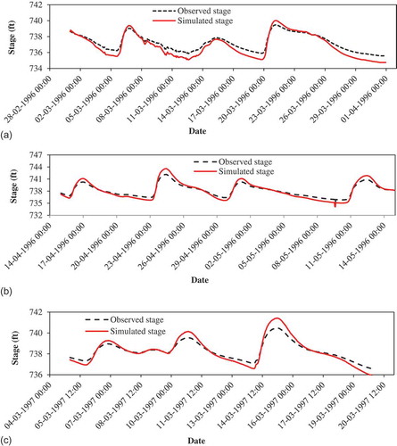
Figure 6. Discharge calibration (a) 1–31 March 1996 and (b) 15 April–14 May 1996, and (c) validation 5–19 March 1997 at downstream gage station 04212100.

5.2 Effect of discharge variation

From the hydraulic analysis for flood discharge of varying return period along with certain variation in discharge, it was found that variation in discharge has a noticeable effect on flood travel time. The variation in discharge was taken to be ±25%, as shown in Table 4. The change in travel time due to the discharge variation was found to be more for negative variation than for positive variation. The detailed results of the analysis are shown in Table 4.

Table 4. Effect on travel time due to the variation in river discharge.

	Change in travel time
Discharge variation	2006 flood	500-year return period	100-year return period	50-year return period	10-year return period	Average change in travel time
−25%	15.71%	16.45%	17.26%	17.85%	19.16%	17.29%
−20%	12.12%	12.47%	13.08%	13.44%	14.44%	13.11%
−15%	8.44%	8.89%	9.27%	9.58%	10.29%	9.29%
−10%	5.38%	5.70%	5.85%	6.06%	6.55%	5.91%
−5%	2.56%	2.66%	2.79%	2.89%	3.12%	2.81%
0%	0.00%	0.00%	0.00%	0.00%	0.00%	0.00%
5%	−2.36%	−2.47%	−2.55%	−2.63%	−2.79%	−2.56%
10%	−4.54%	−4.73%	−4.98%	−5.03%	−5.42%	−4.94%
15%	−6.55%	−6.81%	−7.01%	−7.26%	−7.80%	−7.09%
20%	−8.43%	−8.76%	−9.21%	−9.39%	−10.01%	−9.16%
25%	−10.17%	−10.55%	−11.09%	−11.16%	−12.06%	−11.01%

5.3 Effect of topography

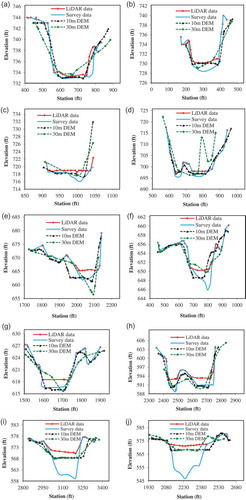
The effect of topography on flood inundation extent depends on the size of the river, bathymetry of the river, and the hydraulic modeling approach (Merwade et al. 2008). The elevation of rivers at different cross-sections varied greatly when different elevation datasets were used. The cross-sections for 10 different locations generated from four different elevation datasets are shown in Figure 7. It was found that, in the majority of those cross-sections, the topographic data represented by the 10-m DEM was better than LiDAR data, particularly in channel sections, indicating that cross-sections generated from the 10-m DEM were better at representing the actual cross-sections. This is not surprising as airborne LiDAR cannot penetrate water (Allouis et al. 2007), especially in the channel sections, which leads to the necessity of bathymetric LiDAR technology. However, LiDAR data are expected to represent the floodplain well, as these data are prepared in high resolution.

Figure 7. Cross-sections at different points along the Grand River: (a) 170 766.4, (b) 167 516.6, (c) 160 741, (d) 146 411.3, (e) 117 638.8, (f) 100 566.7, (g) 71 922.68, (h) 42 626.06, (i) 10 210.82 and (j) 3803.34. Survey data for 10 210.82 and 3803.34 cross-sections have been taken from the survey documents of US Army Corps of Engineers Buffalo District. Survey was performed by a sounding method.

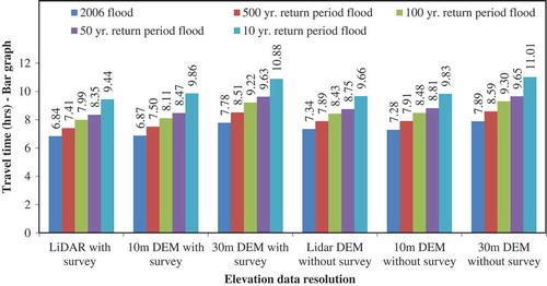
The study found that the travel time for different return period floods varied based on the resolution of the datasets used in the hydraulic analysis. Travel times to reach the City of Painesville and Fairport Harbor for four different return period floods and the 2006 flood were calculated using six different elevation datasets. The graphical representation of travel time and percentage difference in travel time for various return period floods to reach the City of Painesville are shown in Figure 8. The calculated travel time was found to be highest for the most coarse elevation dataset (30-m DEM without survey) and was of decreasing order for finer elevation datasets with the exception of LiDAR data. For example, the maximum difference in calculated travel time for various return period floods was 11.03–15.01% for the 30-m DEM without integration of survey data and the minimum was 1.19–3.35% for the 10-m DEM integrated with survey data. It is interesting to note that the 10-m DEM without integrating the survey data revealed small differences in travel time to the City of Painesville when compared to the travel time computed using LiDAR data without survey. The percentage difference for the 10-m DEM without survey was 3.67–4.87%, whereas it was 10.24–11.75% for LiDAR without survey. A similar pattern was detected for the case of travel time from Harpersfield to Fairport Harbor. The graphical representation of travel time and percentage error in travel time for different return period floods to reach Fairport Harbor is shown in Figure 9. There was a maximum difference of 13.29–14.28% in calculated travel time for the 30 m DEM without integration of survey data for various return period floods. However, a minimum difference of 0.50–4.33% was detected for the 10-m DEM integrated with survey data (Fig. 9). The calculated travel time for LiDAR data without integration of survey data was relatively higher. One of the reasons for this could be the coarser elevation data in channel sections as airborne LiDAR data cannot penetrate water bodies to accurately portray the river bed elevation. Similarly, the water surface elevation and total flow area for LiDAR data without integration of survey data were also found to be higher than some other coarser elevation datasets. Consequently, the flow and computed velocity were relatively smaller, resulting in higher travel time. Therefore, we also conclude, as did earlier findings, that bathymetric data are absolutely needed for the appropriate representation of river profiles. Since bathymetric LiDAR data were not available, a detailed survey was conducted along the channel sections to modify the cross-section, and best represent the site conditions in the model. The river cross-sections after detailed survey were incorporated in the LiDAR data in channel sections. This decreased the travel time to reach the City of Painesville by 10.24–11.75% (Fig. 8) and by 2.33–6.84% to reach Fairport Harbor for various return period floods (Fig. 9).

Figure 8. Travel time and difference in travel time for different return period floods to reach the City of Painesville using different elevation datasets. Percentage decrease/increase in travel time and inundation area for different elevation datasets was computed by comparing with the results calculated using LiDAR with survey.

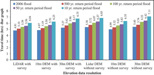
Figure 9. Travel time and percentage difference in travel time for different return period floods to reach Fairport Harbor using different elevation datasets.

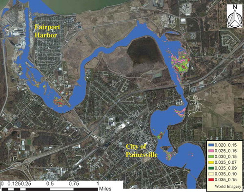
Furthermore, inundation maps were also generated for five different return period floods using six elevation datasets. The graphical representation of inundation area, including its percentage difference for different return period floods and different elevation datasets, is shown in Figure 10. It was found that the inundation area increased with the coarser resolutions of elevation datasets. For example, the inundation area for the 500-year return period flood using LiDAR data with survey was 4.10 square miles (10.62 km²), and using the 30-m DEM without survey it was 5.55 square miles (14.4 km²), with an area difference of 35.37%. The maximum difference in inundation was found to be 32.56–44.52% for the 30-m DEM without integration of survey data for various return period floods, and the minimum difference was 3.55–7.80% for the 10-m DEM when integrated with survey data (Fig. 10). The flood inundation maps of the 2006 flood period were generated using various elevation datasets to have a clear picture of inundation area difference. These flood maps were generated in HEC-GeoRAS and the difference in inundation area is shown in Figure 11. The primary reason for the inundation difference was found to be because of higher predicted water surface elevation for elevation datasets having coarse resolution (which is the 30-m DEM without integration of survey in this study). The importance of detail bathymetry data to generate inundation maps was clearly observed. When the bathymetry data (survey data) were incorporated in the DEM, a decrease in predicted inundation area was observed. The average reduction in inundation area of five different return period floods was found to be highest (17%) for the 30-m DEM and least (9%) for LiDAR (Table 5). This finding was consistent with the results presented by Merwade et al. (2008).

Table 5. Decrease in inundation area when survey data are incorporated.

Return period flood	LiDAR data	10-m DEM	30-m DEM
2006 flood	7.48%	9.73%	16.38%
500-year	7.45%	8.87%	16.40%
100-year	8.43%	10.44%	16.92%
50-year	9.02%	11.27%	17.50%
10-year	13.41%	12.30%	17.86%
Average decrease	9.16%	10.52%	17.01%

Figure 10. Inundation area and percentage difference in inundation area for different return period floods and elevation datasets. Percentage decrease/increase in travel time and inundation area for different elevation datasets was computed by comparing with the results calculated using LiDAR with survey.

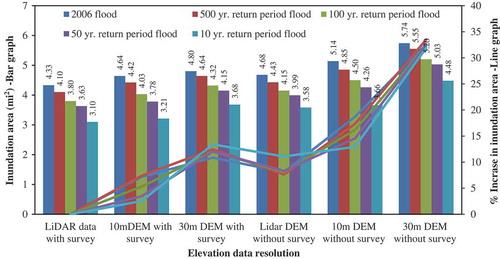
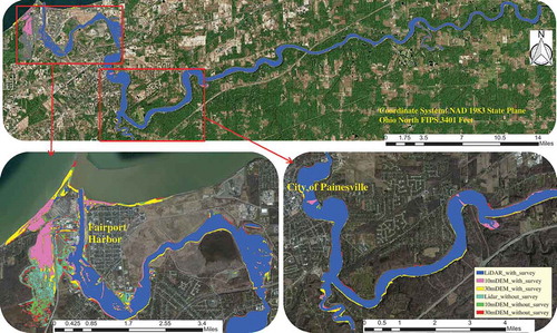
Figure 11. Difference in inundation area due to 2006 flooding in the Grand River generated using different elevation datasets. Note: The pink on the map covers all areas shaded in pink as well as blue; the yellow covers all areas in blue, pink and yellow, and the red represents the 30-m DEM without survey showing areas shaded in red and all the areas that are included in all other cases.

Also, we compared the top width and the flow area for the 2006 flood at several locations on the river. In most cases, there was a decrement in top width and flow area after the integration of bathymetry data. The decrement percentage was higher for the 30-m DEM and least for LiDAR data. Moreover, there was an increase in channel velocity and total average velocity which resulted in decreasing travel time for various return period floods when survey data were incorporated.

5.4 Effect of Manning’s roughness

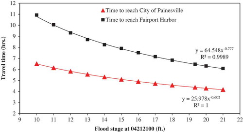
As stated earlier, the results showed the difference in travel time and inundation maps when series of different Manning’s roughness values were used. In this study, five different return period floods on the Grand River were analyzed in two different ways. First, we considered the constant value of roughness in the channel section while varying the roughness value in the floodplains. Four different roughness values (0.15, 0.10, 0.09 and 0.07) within acceptable range were chosen to see the variation. The detailed results of travel time to the City of Painesville for different values of Manning’s roughness are presented in Table 6. The lower values of Manning’s roughness in the floodplains resulted in increased travel times although the increment was not significant. The maximum increment was found to be 3.45% for the 2006 flood when the roughness value was the lowest (0.07) among the four different values (Table 6). Second, a constant value of roughness was considered in the floodplains and a varied value in channel sections. For this, four different possible roughness values (0.035, 0.030, 0.025 and 0.020) in channel sections were chosen. As the roughness value was lowered in channel sections, there was a significant decrease in travel time for different return period floods. The maximum decrement ranged from 20.72 to 22.35% when the roughness value was 0.020 at a channel section (Table 6). The main reason for the decrement was an increase in channel flow velocity due to a decrease in roughness value. The travel time to reach the City of Painesville and Fairport Harbor for the various flood stages at gage station 04212100 is shown in Figure 12. The graph shows how the flood travel time varies depending upon the nature of flood magnitude. We simply computed travel time using velocity and cross-sectional area. This is one limitation of the steady state approach.

Table 6. Travel time to City of Painesville for different Manning’s roughness (n) values.

		Percentage increase or decrease in n (channel, floodplain)^a.b
Return period flood	Travel time (h) for n = 0.035, 0.15	0.035, 0.10	0.035, 0.09	0.035, 0.07	0.030, 0.15	0.025, 0.15	0.020, 0.15
2006 flood	4.81	1.52	2.02	3.45	–7.48	–14.32	–20.72
500-year	5.10	1.04	1.55	2.75	–7.59	–14.48	–20.98
100-year	5.39	0.95	1.32	2.27	–7.61	–14.60	–21.12
50-years	5.56	0.82	1.13	2.00	–7.67	–14.74	–21.42
10-year	6.04	0.60	0.84	1.48	–7.77	–15.19	–22.35

^aIn percentage increase/decrease, the first three columns show the results when n is varied in the floodplain while constant in the channel; the last three columns show the results when n is varied in the channel while constant in the floodplain.

^bNegative sign indicates the percentage decrease.

Figure 12. Travel times for various flood stages in the Grand River to reach the City of Painesville and Fairport Harbor.

Similarly, the effect of Manning’s roughness was observed in inundation area as well. Floodplain maps were produced for different sets of roughness values in channel and floodplain regions. There was a decrease in flood inundation area for lower values of Manning’s roughness than those of the calibrated/validated values. The percentage decrease in inundation area when using different values of Manning’s roughness is shown in Figure 13. In the first case (roughness value was lowered in the floodplain region but kept constant at the channel), the decrease in inundation area was less than 1.49%. However, in the second case (roughness value was lowered in the channel but kept constant in the floodplain region), the decrease in inundation area was 8.97% (Fig. 13). The sensitivity of roughness in floodplain mapping was found to be higher in the second case. The decrease in inundation area was noticed mostly in the flat regions along the river. This does not necessarily mean a large decrement of water surface level in flat regions, but the major reason for a noticeable decrement in inundation area in flat regions was because a small drop of water surface level in flat regions results in a larger difference in inundation area. Therefore, the appropriate calibration of Manning’s roughness at channel sections is more crucial. The difference in predicted inundation area for different Manning’s roughness is shown in Figure 14. While we conducted 2D unsteady flow simulation and compared it with a 1D model, the average difference in predicted discharge was less than 5% in most of the periods (1997–1998).

Figure 13. Percentage decrease in inundation area for different values of Manning’s roughness.

Figure 14. Differences in flood inundation maps for different Manning’s roughness values.

6 Conclusion

Accurate floodplain maps are essential tools for floodplain managers and insurance actuaries to make appropriate decisions to plan rescue operations in affected areas during flooding periods. In this paper, the effects of the resolution of topographic datasets and Manning’s roughness values in the prediction of flood travel time and inundation areas have been discussed. Five different floods were considered for analysis: 10-, 50-, 100- and 500-year return period floods and the 2006 flood. These different floods were simulated in a widely recognized hydraulic model, HEC-RAS, using various topographic datasets and a wide range of Manning’s roughness. A topographic survey was carried out to represent an accurate elevation dataset in the river channel sections, assuming that LiDAR data give the correct elevation representation, especially in the floodplain. The surveyed elevation datasets were integrated with high-resolution LiDAR data. Among all the elevation datasets, the travel time was highest for the coarse data (30-m DEM without integration of survey data) and had a decreasing trend for the high-resolution data. However, the calculated travel time obtained from 10-m DEM without integration of survey data showed less difference than the result obtained from LiDAR without integration of survey. Therefore, it can be concluded that the elevation data in channel section may be better represented by the 10-m DEM than LiDAR when field survey data are not available. However, the predicted inundation area from LiDAR without survey had less area difference than that of the 10-m DEM without survey. Nevertheless, a topographic survey is required to get an actual representation of the land surfaces in channel sections.

In this study, LiDAR with the integration of survey data gave conservative travel times. Since it is always safe to make a decision based on the worst case scenario, lesser travel times would be appropriate for planning evacuation from the possible inundation areas. Similarly, the predicted area of inundation also increased as the coarser resolution of datasets was used, and the percentage difference was very high for the 30-m DEM without integration of survey. Therefore, it can be concluded that the very coarse dataset considered in this study (30-m DEM without integration of survey data) is not appropriate for the calculation of travel times and the generation of flood inundation maps. The differences in travel time and inundation area results were substantial in the 30-m DEM even after the integration of survey data. It was also found that there were decrements in travel time, inundation area, flow area and top width flow and an increment in the velocity of flow when the bathymetry data were integrated to any resolution of dataset. Therefore, when coarse datasets are used for travel time computation and generation of flood inundation maps, some factor of safety should be considered to take into account the possible errors that may be related to travel time, inundation area, flow velocity and top flow width.

The effect of Manning’s roughness was found to be more crucial in flood travel time computation and prediction of inundation area, especially in channel sections. As the value of roughness in the channel sections was decreased, there was a significant decrease in flood travel time (up to 22.35%) and decrease in inundation area (up to 8.97%). The effect of Manning’s roughness on flood travel time and inundation area was studied only for the 2006 flood event in the City of Painesville, assuming a similar effect in other flood events.

Many other uncertainties might be associated with travel time computation and floodplain mapping. From this perspective, it would be wise to use probabilistic floodplain maps as only part of flood mitigation strategies. Since flood travel time computation is essential to evacuate people from probable inundation areas, it may be appropriate to remain on the conservative side when calculating travel time for early evacuation using calibrated Manning’s roughness and higher resolution data . On the other hand, it would be better to generate flood inundation maps based on a slightly higher value of roughness and higher resolution data so that the affected areas are not underestimated. Hence, slightly underestimated results in travel time and slightly overestimated results in inundation area mapping might be helpful when planning and making flood warning decisions.

It should be noted that the calibration of Manning’s roughness for this study was performed based on unsteady flow simulation. However, the entire results for travel time and inundation maps were obtained based on the steady flow assumption in the HEC-RAS model. The steady flow assumption made in this study, particularly for the high flow period, is valid, and this is general practice in simulating flows in steady state conditions during peak flow time. This study also utilized 2D analysis of unsteady flow using HEC-RAS; however, this did not show a significant difference compared to the result (prediction of discharge) obtained from 1D HEC-RAS. The average difference in predicted discharge was insignificant. This study did not perform 2D steady flow analyses for peak flows because of the limitation of the 2D steady flow capacities of HEC-RAS. Therefore, in future, 2D steady hydraulic models could be developed to find out if there are any discrepancies compared to results obtained from 1D steady flow analysis, if discharge/stage data for all creeks and time series data for Lake Erie level can be obtained. In addition, the possibility of variation of Manning’s roughness with varying floods could be addressed in future to see probable differences in travel times and inundation area. Some errors might be associated with the calculated flows in tributaries of the Grand River, as flows in tributaries were computed using regression equations. This error might be transferred to the hydraulic model resulting in dissipation of further errors in water surface elevation and flood extents.

Disclosure statement

No potential conflict of interest was reported by the authors.

Additional information

Funding

The authors would like to acknowledge support from Ohio Sea Grant System through Ohio State University to conduct this research (R/EM-032) [Grant No. 60055607].

References

- Alho, P. and Aaltonen, J., 2008. Comparing a 1D hydraulic model with a 2D hydraulic model for the simulation of extreme glacial outburst floods. Hydrological Processes, 22 (10), 1537–1547. doi:10.1002/(ISSN)1099-1085
- Allouis, T., Bailly, J., and Feurer, D., 2007. Assessing water surface effects on LiDAR bathymetry measurements in very shallow rivers: a theoretical study. In: Second ESA space for hydrology workshop [online], Geneva, CHE, 12–14. Available from: https://www.researchgate.net/profile/Denis_Feurer/publication/268260522_Assessing_water_surface_effects_on_LiDAR_bathymetry_measurements_in_very_shallow_rivers_a_theoretical_study/links/54bcd6f30cf29e0cb04c390b.pdf
- Arcement, G.J. and Verne, R.S., 1989. Guide for selecting Manning’s roughness coefficients for natural channels and flood plains [online]. Available from: http://dpw.lacounty.gov/lacfcd/wdr/files/WG/041615/Guide%20for%20Selecting%20n-Value.pdf
- ASCE Task Committee, 1993. The ASCE task committee on definition of criteria for evaluation of watershed models of the watershed management committee Irrigation and Drainage Division, Criteria for evaluation of watershed models. Journal of Irrigation and Drainage Engineering, ASCE, 119 (3), 429–442.
- Bales, J.D. and Wagner, C.R., 2009. Sources of uncertainty in flood inundation maps. Journal of Flood Risk Management, 2.2, 139–147. doi:10.1111/j.1753-318X.2009.01029.x
- Barnes Jr., H.H., 1849. Roughness characteristics of natural streams [online]. US Geological Survey Water Supply Paper. Available from: https://pubs.usgs.gov/wsp/wsp_1849/pdf/wsp_1849.pdf
- Basha, E. and Daniela, R., 2007. Design of early warning flood detection systems for developing countries. In: Information and Communication Technologies and Development, 2007. ICTD 2007. International Conference on Information and Communication Technologies and Development, 15–16 December, Bangalore, India, 1–10.
- Bates, P.D., et al., 2004. Bayesian updating of flood inundation likelihoods conditioned on flood extent data. Hydrological Processes, 18 (17), 3347–3370. doi:10.1002/(ISSN)1099-1085
- Bates, P.D. and De Roo, A.P.J., 2000. A simple raster-based model for floodplain inundation. Journal of Hydrology, 236, 54–77. doi:10.1016/S0022-1694(00)00278-X
- Brunner, G.W., 1995. HEC-RAS River Analysis System [online]. Hydraulic Reference Manual. Version 1.0. Davis, CA: US Army Corps of Engineers, Hydrologic Engineering Center. Available from: http://www.dtic.mil/dtic/tr/fulltext/u2/a311952.pdf
- Brunner, G.W., 2002. HEC-RAS river analysis system: user’s manual. Davis, CA: US Army Corps of Engineers, Institute for Water Resources, Hydrologic Engineering Center.
- Castellarin, A., et al., 2009. Optimal cross-sectional spacing in Preissmann scheme 1D hydrodynamic models. Journal of Hydraulic Engineering, 135 (2), 96–105. doi:10.1061/(ASCE)0733-9429(2009)135:2(96)
- Chow, V.T., Maidment, D.R., and Mays, L.W., 1988. Applied hydrology. New York: McGraw-Hill.
- Cook, A. and Merwade, V., 2009. Effect of topographic data, geometric configuration and modeling approach on flood inundation mapping. Journal of Hydrology, 377 (1), 131–142. doi:10.1016/j.jhydrol.2009.08.015
- Cook, A.C., 2008. Comparison of one-dimensional HEC-RAS with two-dimensional FESWMS model in flood inundation mapping. Dissertation. Purdue University West Lafayette.
- Costabile, P., et al., 2015. Flood mapping using LIDAR DEM. Limitations of the 1D modeling highlighted by the 2-D approach. Natural Hazards, 77 (1), 181–204. doi:10.1007/s11069-015-1606-0
- Crosetto, M. and Tarantola, S., 2001. Uncertainty and sensitivity analysis: tools for GIS-based model implementation. International Journal of Geographical Information Science, 15 (5), 415–437. doi:10.1080/13658810110053125
- Di Baldassarre, G., 2012. Flood trends and population dynamics. In: EGU General Assembly Conference Abstracts, 22–27 April, Vienna, Austria.
- Di Baldassarre, G. and Montanari, A., 2009. Uncertainty in river discharge observations: a quantitative analysis. Hydrology and Earth System Sciences, 13 (6), 913. doi:10.5194/hess-13-913-2009
- Domeneghetti, A., et al., 2013. Probabilistic flood hazard mapping: effects of uncertain boundary conditions. Hydrology and Earth System Sciences, 17 (8), 3127–3140. doi:10.5194/hess-17-3127-2013
- Dottori, F., Baldassarre, G.D., and Todini, E., 2013. Detailed data is welcome, but with a pinch of salt: accuracy, precision, and uncertainty in flood inundation modeling. Water Resources Research, 49 (9), 6079–6085. doi:10.1002/wrcr.20406
- Ebner, A.D., et al., 2006. Flood of July 27–31, 2006, on the Grand River near Painesville, Ohio. Reston, VA: US Geological Survey, Open-File Report 2007–1164.
- Fread, D.L., 1974. Numerical properties of implicit four-point finite difference equations of unsteady flow [online]. Washington, DC: Office of Hydrology. Available from: http://www.nws.noaa.gov/oh/hrl/hsmb/docs/hydraulics/papers_before_2009/hl_51.pdf
- Gupta, H.V., Sorooshian, S., and Yapo, O.P., 1999. Status of automatic calibration for hydrologic models: comparison with multilevel expert calibration. Journal of Hydrologic Engineering, 4 (2), 135–143. doi:10.1061/(ASCE)1084-0699(1999)4:2(135)
- Guthrie, J.D., et al., 2008. Stewart.StreamStats: a water resources web application. Reston, VA: US Department of the Interior, US Geological Survey.
- Hicks, F.E. and Peacock, T., 2005. Suitability of HEC-RAS for flood forecasting. Canadian Water Resources Journal, 30 (2), 159–174. doi:10.4296/cwrj3002159
- Holtzclaw, E., Leite, B., and Myrick, R., 2005. Floodplain modeling applications for emergency management and stakeholder involvement a case study. New Braunfels, TX: Georgia Institute of Technology.
- Horritt, M.S. and Bates, P.D., 2001. Effects of spatial resolution on a raster based model of flood flow. Journal of Hydrology, 253 (1), 239–249. doi:10.1016/S0022-1694(01)00490-5
- Horritt, M.S. and Bates, P.D., 2002. Evaluation of 1D and 2D numerical models for predicting river flood inundation. Journal of Hydrology, 268 (1–4), 87–99. doi:10.1016/S0022-1694(02)00121-X
- Jung, H.C., et al., 2011. Analysis of the relationship between flooding area and water height in the Logone floodplain. Physics and Chemistry of the Earth, Parts A/B/C, 36 (7–8), 232–240. doi:10.1016/j.pce.2011.01.010
- Kalyanapu, A.J., Burian, S.J., and McPherson, T.N., 2009. Effect of land use-based surface roughness on hydrologic model output. Journal of Spatial Hydrology, 9 (2), 51–71.
- King, R.O., 2009. National flood insurance program: background, challenges, and financial status. Washington, DC: Congressional Research Service, Library of Congress.
- Koltun, G.F. and Roberts, J.W., 1990. Techniques for estimating flood-peak discharges of rural, unregulated streams in Ohio. Department of the Interior, US Geological Survey, 89, 4126.
- Krimm, R.W., 1996. Reducing flood losses in the United States. In: Proceedings of International Workshop on Floodplain Risk Management, 11–13 November, Hiroshima.
- Krzysztofowicz, R., Karen, S.K., and Dou, L., 1994. Reliability of flood warning systems. Journal of Water Resources Planning and Management, 120 (6), 906–926. doi:10.1061/(ASCE)0733-9496(1994)120:6(906)
- Leedal, D., et al., 2010. Visualization approaches for communicating real‐time flood forecasting level and inundation information. Journal of Flood Risk Management, 3 (2), 140–150. doi:10.1111/jfrm.2010.3.issue-2
- Liggett, J.A. and Jean, A.C., 1975. Numerical methods of solution of the unsteady flow equations. Unsteady Flow in Open Channels, 1 (89), 182.
- Lowe, A.S., 2003. The federal emergency management agency’s multi-hazard flood map modernization and the national map. Photogrammetric Engineering & Remote Sensing, 69 (10), 1133–1135. doi:10.14358/PERS.69.10.1133
- Marks, K. and Bates, P., 2000. Integration of high-resolution topographic data with floodplain flow models. Hydrological Processes, 14 (11–12), 2109–2122. doi:10.1002/(ISSN)1099-1085
- Merwade, V., et al., 2008. Uncertainty in flood inundation mapping: current issues and future directions. Journal of Hydrologic Engineering, 13 (7), 608–620. doi:10.1061/(ASCE)1084-0699(2008)13:7(608)
- Merwade, V., Cook, A., and Coonrod, J., 2008. GIS techniques for creating river terrain models for hydrodynamic modeling and flood inundation mapping. Environmental Modelling & Software, 23 (10–11), 1300–1311.
- Merz, B.A., Thieken, H., and Gocht, M., 2007. Flood risk mapping at the local scale: concepts and challenges. In: Flood risk management in Europe. Dordrecht: Springer, 231–251.
- Moriasi, D., et al., 2007. Model evaluation guidelines for systematic quantification of accuracy in watershed simulations. Transactions of the ASABE, 50 (3), 885–900. doi:10.13031/2013.23153
- Nash, J.E. and Sutcliffe, J.V., 1970. River flow forecasting through conceptual models part I—A discussion of principles. Journal of Hydrology, 10 (3), 282–290. doi:10.1016/0022-1694(70)90255-6
- Oegema, B.W. and McBean, E., 1987. A. Uncertainties in flood plain mapping. In: Application of frequency and risk in water resources. Dordrecht: Springer, 293–303.
- Ohio Department of Administrative Services, 2007. Ohio Statewide Imagery Program [online]. Available from: http://ogrip.oit.ohio.gov/
- Ostheimer, C.J., 2012. Development of a flood-warning system and flood-inundation mapping in Licking county, Ohio. Reston, VA: US Geological Survey, No. FHWA/OH-2012/4.
- Pappenberger, F., et al., 2005. Uncertainty in the calibration of effective roughness parameters in HEC-RAS using inundation and downstream level observations. Journal of Hydrology, 302 (1–4), 46–69. doi:10.1016/j.jhydrol.2004.06.036
- Pappenberger, F., et al., 2006. Influence of uncertain boundary conditions and model structure on flood inundation predictions. Advances in Water Resources, 29 (10), 1430–1449.
- Parhi, P.K., Sankhua, R.N., and Roy, G.P., 2012. Calibration of channel roughness for Mahanadi River, (India) using HEC-RAS model. Journal of Water Resource and Protection, 4 (10), 847. doi:10.4236/jwarp.2012.410098
- Perry, C.A., 2000. Significant floods in the United States during the 20th century-USGS measures a century of floods. Reston, VA: US Geological Survey, No. 024-00.
- Pilgrim, D.H., 1976. Travel times and nonlinearity of flood runoff from tracer measurements on a small watershed. Water Resources Research, 12 (3), 487–496.
- Re, M., 2011. Great natural catastrophes worldwide 1950–2010. Munich, Germany: Münchener Rückversicherungs-Gesellschaft, Geo Risks Research, NatCatSERVICE.
- Samuels, P.G., 1990. Cross-section location in 1D models. In: W.R. White, ed. Proceedings of International Conference on River Flood Hydraulics. Chichester: John Wiley, 339–350.
- Sanders, B.F., 2007. Evaluation of on-line DEMs for flood inundation modeling. Advances in Water Resources, 30 (8), 1831–1843.
- Smemoe, C., Nelson, J., and Zundel, A., 2012. Developing a probabilistic flood plain boundary using HEC-1 and HEC-RAS. In: World Water and Environmental Resources Congress 2003, 23–26 June 2003, Philadelphia, PA. doi:10.1061/40685(2003)286
- Tayefi, V., et al., 2007. A comparison of one‐and two‐dimensional approaches to modelling flood inundation over complex upland floodplains. Hydrological Processes, 21 (23), 3190–3202. doi:10.1002/(ISSN)1099-1085
- Timbadiya, P.V., Patel, P.L., and Porey, P.D., 2011. Calibration of HEC-RAS model on prediction of flood for lower Tapi River, India. Journal of Water Resource and Protection, 3 (11), 805. doi:10.4236/jwarp.2011.311090
- USACE (US Army Corps of Engineers), 2000. Revised report on Great Lakes open-coast flood levels [online]. Detroit, MI: USACE. Available from: https://www.michigan.gov/documents/deq/wrd-nfip-great-lakes-flood-levels-part1_564793_7.pdf
- Whitehead, M.T. and Ostheimer, C.J., 2009. Development of a flood-warning system and flood-inundation mapping for the Blanchard river in Findlay, Ohio. Reston, VA: US Geological Survey, No. 2008-5234.