A continuous modelling approach for design flood estimation on sub-daily time scale

ABSTRACT

Design flood estimation is an essential part of flood risk assessment. Commonly applied are flood frequency analyses and design storm approaches, while the derived flood frequency using continuous simulation has been getting more attention recently. In this study, a continuous hydrological modelling approach on an hourly time scale, driven by a multi-site weather generator in combination with a $k$-nearest neighbour resampling procedure, based on the method of fragments, is applied. The derived 100-year flood estimates in 16 catchments in Vorarlberg (Austria) are compared to (a) the flood frequency analysis based on observed discharges, and (b) a design storm approach. Besides the peak flows, the corresponding runoff volumes are analysed. The spatial dependence structure of the synthetically generated flood peaks is validated against observations. It can be demonstrated that the continuous modelling approach can achieve plausible results and shows a large variability in runoff volume across the flood events.

KEYWORDS:

• derived flood frequency
• continuous modelling
• temporal disaggregation
• flood hazard
• synthetic flood events

Editor A. Castellarin Associate editor E. Volpi

1 Introduction

Flooding is associated with severe negative consequences to society, the economy and human health. For flood risk assessment and management, information about possible extreme floods, e.g. about an event with a return period of 100 years, is essential (e.g. EU 2007). Therefore, event characteristics need to be derived to serve as a basis for inundation mapping, risk zoning or the design of flood defence infrastructure. While estimates usually refer to the discharge magnitude, the severity of a flood is also defined by the duration and runoff volume of a flood event (Mediero et al. 2010, Grimaldi et al. 2012b, Lamb et al. 2016, Brunner et al. 2017

There are different approaches for design flood estimation. Following the classification of Rogger et al. (2012a), they can be divided into statistical methods, deterministic methods and a combination of the two, which is also referred to as a “derived flood frequency” approach. Flood frequency analysis (FFA), where the design flood is estimated by fitting a theoretical extreme value distribution to observed gauging data, is a commonly applied statistical approach and well established (Robson and Reed 1999, Blöschl et al. 2013). Further, deterministic design storm approaches (DSA) are applied, where predefined design rainfall events are transformed to corresponding discharge using a deterministic rainfall–runoff model. Typically, the critical rainfall duration needs to be identified for the catchment and different temporal rainfall patterns can be tested (Grimaldi et al. 2013). As a combination of statistical and deterministic methods, derived flood frequency analysis based on the continuous simulation of flood flows is the subject of recent research (Haberlandt et al. 2011, Hundecha and Merz 2012, Rogger et al. 2012a, Grimaldi et al. 2012b, Breinl 2016, Arnaud et al. 2017). The continuous modelling approach (CMA) is understood as the continuous hydrological simulation driven by long meteorological time series generated for example by a stochastic weather generator (Blazkova and Beven 1997, 2004, Rogger et al. 2012a, Grimaldi et al. 2013, Lamb et al. 2016). The term “derived” refers to the indirect derivation of the design flood from the resulting synthetic runoff series, typically by means of extreme value statistics (Sivapalan et al. 2005). In this study, the CMA does not include the continuous simulation on observed meteorological data, which can be a valuable method for flood estimation at ungauged locations (Viviroli et al. 2009).

Each of the three methods has its advantages and disadvantages. Flood frequency analysis is easy to apply, but restricted to gauged catchments with sufficiently long time series, though regional flood frequency analysis can be deployed also for ungauged locations (Hosking and Wallis 1997). Usually univariate frequency analysis on peak discharge is utilized (Maniak 2010). To extend the concept to further flood characteristics such as flood volume, multivariate models need to be applied, to account for their dependence (e.g. Serinaldi and Grimaldi 2011, Brunner et al. 2017). In engineering practice, design storm approaches are often used to consider flood volume, as event hydrographs are generated directly, by the transformation of design storm to discharge (Viglione and Blöschl 2009, Rogger et al. 2012a). Design storm approaches can be applied in ungauged basins, but this relies on the assumption of the identity of the return period between rainfall and resulting peak discharge, which remains questionable (Viglione et al. 2009). Further, the pre-event catchment state and the critical storm duration are usually defined rather subjectively (Boughton and Droop 2003). The latter limitations are overcome with the continuous simulation approach (Grimaldi et al. 2013). The downside, however, is that the CMA is complex and computationally intensive and therefore seldom applied in practical applications (Rogger et al. 2012a). Furthermore, by the involvement of multiple models, additional sources of uncertainties are introduced (Arnaud et al. 2017). The CMA can, however, be applied with limited observed streamflow data, or if knowledge about flood frequencies is needed at multiple locations in a catchment (Haberlandt et al. 2011). With the generation of long time series, the sampling uncertainty may be reduced, as so far unobserved meteorological conditions and catchment states are included (Rogger et al. 2012b). Additionally, continuous simulations are promising because of their potential to link physical processes, to avoid rather subjective assumptions (e.g. the pre-event catchment state and critical storm duration) and to provide full hydrograph characteristics (Lamb et al. 2016). By the inclusion of physical processes, the CMA can also be applied for impact and attribution studies of climate and land-use change (Holzmann et al. 2010, Hundecha and Merz 2012, Breinl 2016).

Recently, only a small number of studies have dealt with the comparison of continuous modelling approaches to FFA and DSA. Grimaldi et al. (2012b) compared simulated peak discharge, event durations and runoff volume between continuous simulations and a design storm approach. While spatially uniform rainfall was generated on a 5-min resolution in the study, the transformation from precipitation pursues a unit hydrograph approach without detailed process descriptions. By directly linking the methods to hydraulic simulations, the effect on inundation modelling was analysed, showing that event-based models may underestimate flood volumes (Grimaldi et al. 2013). A comprehensive comparison between FFA, DSA and CMA was presented by Rogger et al. (2012a). The meteorological input was generated by a stochastic point rainfall generator on a sub-hourly scale and combined with observed temperatures to estimate flood frequency. A recent study by Breinl (2016), with the focus on exploring the effect of differently complex weather generators, concluded that FFA and CMA can achieve comparable results on a daily scale. The CMA studies were limited to either single-site applications on sub-daily time scale (Grimaldi et al. 2012b, 2013, Arnaud et al. 2017) or multi-site applications on a daily time scale (Hundecha and Merz 2012, Falter et al. 2015, Breinl 2016, Breinl et al. 2017).

In contrast, this study aims to apply a spatially coherent continuous modelling approach at an hourly time scale for estimating low-frequency flood events (e.g. 100-year floods) in small mountainous catchments that react rather quickly. Another objective is to compare the modelling results to the flood frequency analysis of gauge data and a design storm approach. For the DSA and CMA, corresponding event volumes are also compared besides peak discharge. In this study, the CMA encompasses a daily multi-site, multi-variate weather generator and a disaggregation procedure at the hourly time scale, which provides the meteorological boundary conditions to a semi-distributed hydrological model.

This paper is organized in six sections. Firstly, the study area and data are described. Secondly, the approaches for design flood estimation are explained with a comprehensive description of the model chain for continuous simulation. In Section 4, the results of the continuous model chain are presented. The outcomes of the different approaches are compared and discussed, including their limitations, in Section 5 and, finally, a summary is provided and conclusions are drawn.

2 Study area and data

The study was conducted in the Austrian Federal Province of Vorarlberg. In total, 16 catchments with areas ranging from 25 to 1277 km² were analysed (Table 1). The settlement areas, covering about 5% of Vorarlberg, are mainly concentrated in the valley floors, making them vulnerable to flooding. The predominant land-cover types are extensively managed grasslands and deciduous and coniferous forests, which cover about 40% of the study area. The morphology varies from the flat Rhine valley, with the lowest altitude of approx. 400 m a.s.l., to high mountain reaches with an altitude above 3000 m a.s.l. in the headwater catchments of the Bregenzerach (BA) and Ill (IL) rivers. The average terrain slopes range from 6° in the northernmost pre-alpine catchment of the Leiblach (LB) River up to 28.2° in the alpine drainage area of the Lutz River at the gauge Garsella. On average, the slope is above 20°, resulting in a fast hydrological response with short runoff concentration times, especially for the small headwater catchments of the Lech (LE) and Frutz (FU). In particular, some headwater catchments and the southern tributaries of the Ill River are influenced by hydropower operations. Strongly influenced headwater catchments were not selected for this study. At the gauges Gisingen and Kennelbach, which are located at the outlets of the Ill and Bregenzerache catchments, respectively, the entire discharge used for hydropower operations within the catchments is returned to the rivers. The discharge series are at most 63 years long, starting from 1951, with the shortest series of 24 years at the gauge Bürs. Table 1 lists the study catchments together with the catchment areas and the length of the discharge time series.

Table 1. List of study catchments together with catchment area and length of the observed discharge time series

Gauge	River	Basin	Catchment area (km^2)	Length of discharge series (years)
Au	Bregenzerach	BA	149.3	63
Hopfreben	Bregenzerach	BA	40.8	57
Kennelbach	Bregenzerach	BA	825.2	63
Mellau	Bregenzerach	BA	226.9	63
Thal Martinsbrück	Rotach	BA	85.3	53
Enz	Dornbirnerach	DA	53.7	58
Hoher Steg	Dornbirnerach	DA	113.6	58
Lauterach	Dornbirnerach	DA	201.4	31
Laterns	Frutz	FU	33.4	58
Bürs	Alvier	IL	74	24
Garsella	Lutz	IL	94	50
Gisingen	Ill	IL	1277	62
Schruns	Litz	IL	98.4	55
Unterhochsteg	Leiblach	LB	109.4	38
Lech Tannbrück	Lech	LE	85.2	63
Lech	Zuersbach	LE	25.1	43

Vorarlberg is characterized by high precipitation amounts due to its location in the northern reaches of the Alps, with predominantly westerly flows and strong orographic effects. Whereas the Ill catchment is partly located in the rain shadow of high alpine ranges, the Bregenzerach and Dornbirnerach (DA) catchments experience precipitation amounts of up to 3000 mm year⁻¹ (BMLFUW 2007). Daily precipitation amounts of more than 200 mm were measured during flood events in the last decades (e.g. station Innerlaterns: 228 mm, 22 August 2005; station Schönenbach: 236 mm, 21 May 1999). In this study, 45 meteorological stations with daily time series from 1971 to 2013 were used. In contrast, data for only 23 sites starting from 2001 are available at hourly time steps. The lack of sub-daily meteorological input data is a common limitation for modelling applications (Förster et al. 2016). Data for stations without hourly data were interpolated by an inverse distance-weighting scheme (see Section 3.3.3). Figure 1 provides an overview of the study catchments, showing the locations of the river gauging stations as well as the meteorological stations.

Figure 1. The study area of Vorarlberg including catchment boundaries, gauging stations and meteorological stations

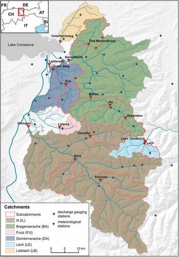
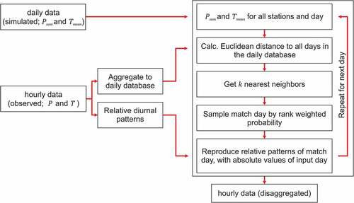
Figure 2. Flowchart of the disaggregation procedure for precipitation and temperature data

3 Methods

Three different approaches for design flood estimation were applied in this study: (1) flood frequency analysis; (2) a design storm approach; and (3) a continuous modelling approach. Besides the description of the approaches, the methodology for the spatial dependence analysis of observed and simulated peak flows and for the event separation for volume calculation is given.

3.1 Flood frequency analysis

Statistical flood frequency analysis (FFA), where a theoretical extreme value distribution is fitted to the observed gauging data, is usually applied if long enough streamflow records are available (Rogger et al. 2012a). In this study, the three-parameter generalized extreme value (GEV) distribution was used. The estimation is based on the annual maximum series (AMS). The GEV is widely used for AMS series (Coles 2001) and has been found suitable for national flood discharge mapping in Austria (Merz et al. 2008). Further, the ${\chi }^2$ goodness-of-fit test was applied. The frequency distributions were fitted using the method of L-moments (Hosking and Wallis 1997). Confidence intervals for the 100-year flood were estimated by means of a percentile confidence interval bootstrapping procedure (e.g. Burn 2003). In contrast to non-parametric bootstrapping (resampling with replacement), the randomly generated sample is derived from the parametric model distribution, which is preferable for smaller sample sizes (Kyselý 2008).

3.2 Design storm approach

The design storm approach (DSA) is based on the transformation of a defined design storm into the corresponding river runoff. This method is mostly applied in engineering hydrology when limited streamflow data are available or large return periods are of interest (Viglione and Blöschl 2009). The design storm is derived from the intensity–duration–frequency (IDF) curve for maximum rainfall intensities of the selected return period (Blöschl et al. 2013). Depending on the characteristics of the catchment, the critical intensity–duration rainfall needs to be defined. Commonly, rather simple event-based rainfall–runoff models are used to transform the design storms into streamflow (Rogger et al. 2012a, Blöschl et al. 2013, Haberlandt and Radtke 2014).

The design storms, or more precisely the IDF curves for the Austrian design storms, were provided by the Austrian Hydrographic Service. They are derived by a combination of (1) a dataset based on the maximum precipitation of an atmospheric model, and (2) a dataset generated by spatially interpolated, extreme value statistics of meteorological station data (Weilguni 2009). In order to account for the assumption of uniform rainfall intensity across the catchment, the design rainfall based on the IDF curves needs to be reduced for larger catchments (Blöschl 2009). For Austria, different empirical formulas are recommended to define the catchment-specific areal reduction factor ($\mathrm{A}\mathrm{R}\mathrm{F}$) (BMLFUW 2011). The empirical ARF considers the catchment size ($A$) and duration ($D$) of the design precipitation as follows (BMLFUW 2011):

(1) $\mathrm{A}\mathrm{R}\mathrm{F}={\mathrm{e}}^{-h{A}^{0.5}}$(1)

where $h$ is defined as:

(2) $h=D^{-0.43}$(2)

The possible temporal variability of the design events is taken into account by four different temporal patterns (DVWK 1984). These include the equally distributed intensity, also called block rainfall, and the temporal allocation of the maximum precipitation intensity (a) at the beginning of an event (start-emphasized), (b) in the middle of an event (middle-emphasized), and (c) at the end of an event (end-emphasized).

The critical intensity–duration was defined by the approximated concentration time resulting in the highest discharge. Four different formulas to calculate the concentration time were considered for each catchment: (i) Department of Public Works, (ii) Giandotti, (iii) Kirpich and (iv) Viparelli (Grimaldi et al. 2012a).

The rainfall–runoff model HQsim was used for the design storm estimation (detailed model description is given in Section 3.3.4). The pre-event conditions are defined as follows: first, the month with the highest occurrence of annual peaks is identified based on observed data. In the next step, runoff is simulated (HQsim) driven by observed hourly input. Then the dates of the 0.1, 0.5 and 0.9 quantiles of simulated streamflow of the selected month are determined. Finally, the model states (e.g. storages) of the identified dates are defined as the pre-event conditions of lower (p = 0.1), median (p = 0.5) and upper (p = 0.9) scenarios. The procedure assumes that the simulated runoff of the catchment reflects the “severity” of pre-event storage conditions. By analysing only the month of highest flood occurrence, the strong seasonality of the study area, with predominant summer floods, will be taken into account.

3.3 Continuous modelling approach

In this study, the continuous simulation of streamflow for design flood estimation includes the following steps: (1) simulation of long series of daily meteorological data using a stochastic weather generator; (2) temporal disaggregation of daily meteorological data to hourly series; and (3) deterministic modelling of streamflow by a semi-distributed rainfall–runoff model. Finally, the 100-year flood was estimated by applying flood frequency statistics to the simulated streamflow data.

3.3.1 Weather generator

For the continuous simulation, a long-term series of meteorological data is generated with a multi-site, multi-variate weather generator on a daily time step (Hundecha et al. 2009, Hundecha and Merz 2012). The two-step model is based on climate station data and is fitted for each month of the year to account for the seasonal characteristics, as well as the temporal and spatial correlations between the different stations. In the first step, the distribution of daily precipitation amounts is modelled for each site by a mixture of two distributions (gamma and generalized Pareto), with dynamically varying weights, with the objective of characterizing the extremes of daily rainfall (Vrac and Naveau 2007). The local occurrence and amount of precipitation are modelled using a multi-variate autoregressive model considering the inter-site dependencies by the autocorrelation and spatial covariance between stations. In a second step, the mean temperature is modelled conditioned on precipitation. The weather generator was applied for hydrological change attribution and flood risk studies in Germany (Hundecha and Merz 2012, Falter et al. 2015). For a more detailed technical description of the weather generator see Hundecha et al. (2009) and Hundecha and Merz (2012).

3.3.2 Disaggregation procedure

In catchments with short concentration times, peak flows can be considerably higher than the daily averages (Dastorani et al. 2013). Due to the small scale of the investigated catchments, their mostly alpine topography and, therefore, short response times, a sub-daily time step is necessary to estimate meaningful peak discharges. Since the weather generator delivers daily data, a temporal disaggregation procedure needs to be applied. As it is difficult to model hourly data directly by stochastic weather generators, the application of subsequent disaggregation techniques is a common bypass (Haberlandt et al. 2011, Pui et al. 2012). In recent years, different methods have been developed to disaggregate daily rainfall to sub-daily time steps. They include resampling techniques based upon the method of fragments (Buishand and Brandsma 2001, Sharma and Srikanthan 2006, Leander and Buishand 2009, Pui et al. 2012, Westra et al. 2013, Breinl et al. 2017), multiplicative cascade models (Olsson 1998, Güntner et al. 2001, Haberlandt and Radtke 2014, Förster et al. 2016, Müller and Haberlandt 2018), and more complex stochastic disaggregation procedures, for example based on the Bartlett-Lewis rectangular pulse model (Koutsoyiannis et al. 2003, Kossieris et al. 2016).

For the present study, a non-parametric resampling procedure was chosen to disaggregate the generated daily values. Pui et al. (2012) showed that resampling techniques can outperform more sophisticated models in terms of observed rainfall statistics, such as wet spells, intensity–frequency relationships and extreme values. Considering this, a k-nearest neighbour algorithm (k-NN) based on the method of fragments was applied to disaggregate daily data to hourly data while keeping the inter-site correlations. The applied disaggregation method follows, generally, the modelling steps proposed by Lall and Sharma (Sharma and Srikanthan 2006). In contrast to other resampling procedures (Sharma and Srikanthan 2006, Nowak et al. 2010, Pui et al. 2012, Breinl et al. 2017), the temperature is disaggregated simultaneously to the precipitation. The course of temperature during the day is thereby expressed as relative difference to daily mean temperature. Aside from the need for hourly temperature inputs, temperature can help to distinguish between long-lasting advective wet spells and intensive convective storms with short duration in the summer months. The disaggregation procedure comprises the following steps (Fig. 2):

1. An observed daily database is prepared by aggregation of hourly data to daily precipitation sums (P_sum) and mean daily temperatures (T_mean).

2. The corresponding relative diurnal patterns are prepared for the precipitation (fragments) and temperature (difference relative to T_mean).

3. For the day to disaggregate, the daily values (simulated P_sum and T_mean) of all stations are taken simultaneously.

4. All days in the observed database (Step 1) of the same month and identical wet or dry state as the day to disaggregate are selected as possible nearest neighbours.

5. The Euclidean distance between the input day and all selected comparison days is calculated for P and T.

6. The calculated distances ($\mathrm{\Delta }P$ and $\mathrm{\Delta }T$) are normalized by their data range to make them comparable.

7. The k-nearest neighbours are identified by the minimal distance ($\mathrm{\Delta }P$ + $\mathrm{\Delta }T$), while the number of neighbours $k$ is defined by the number $n$ of comparison days $k=\sqrt{n}$, according to Lall and Sharma (1996).

8. A rank-weighting scheme ($w$)$:w=\frac{1}{i}/{\sum }_{i=1}^k\frac{1}{i}$, is applied to the k-nearest neighbours, where $i$ refers to the neighbour’s index (Lall and Sharma 1996, Nowak et al. 2010).

9. The match day is randomly sampled by the weighting probability defined in Step 8.

10. The relative temporal patterns from the match day are transferred to the input daily precipitation sums and mean temperature.

11. Steps 3–10 are repeated for all input days.

3.3.3 Spatial interpolation of meteorological variables

As the generation of meteorological data is carried out at the locations of weather stations (point scale), a spatial interpolation is needed for the subsequent application of the semi-distributed rainfall–runoff model.

Many approaches of different complexity exist, such as simple Thiessen polygons, inverse distance weighting, spline interpolation or various kriging methods (Goovaerts 2000, Bavay and Egger 2014, Plouffe et al. 2015). The choice of an adequate algorithm involves a trade-off between accuracy and efficiency.

For this study, the simple inverse distance-weighting scheme including a stepwise lapse rate was chosen, since a computationally efficient resource-conserving method is needed for the long-term simulation. The spatial interpolation of meteorological point data was carried out using the MeteoIO C++ library (Bavay and Egger 2014). If the lapse rate per time step is not acceptable ($R=0.7$, MeteoIO default), fall-back default values derived from long-term means of the meteorological stations are applied ($T_{\mathrm{l}\mathrm{a}\mathrm{p}\mathrm{s}\mathrm{e}}$ = −0.575°C; $P_{\mathrm{l}\mathrm{a}\mathrm{p}\mathrm{s}\mathrm{e}}$ = 1.95% per 100 m). The identical method was applied consistently for the interpolation of missing hourly variables for the disaggregation procedure.

3.3.4 Rainfall–runoff modelling

The rainfall–runoff model HQsim (Kleindienst 1996, Senfter et al. 2009, Achleitner et al. 2012) was applied to obtain streamflow series at the gauging stations. HQsim can be classified as a semi-distributed conceptual model based on hydrological response units (HRUs). The model is forced by temperature and precipitation data. Snow and rain interception are based on a leaf area index (LAI)-dependent approach. Evapotranspiration is calculated according to the concept of Hamon’s potential evaporation taking into account water availability (Dobler and Pappenberger 2013). Snowmelt is estimated by a degree-day factor, further modified by the vegetation cover and a radiation factor. A contributing area concept is applied to divide between infiltration and surface flow in relation to soil saturation, while the movement of water to the unsaturated soil zone is parameterized by the Mulem-van Genuchten model. Groundwater reservoirs are represented by linear storages. The subsurface runoff generation is approximated by a time–area diagram for each HRU and combined with a river routing scheme using the Rickenmann (1996) flow formula to model the channel flows. A more detailed model description is given by Achleitner et al. (2009) and Dobler and Pappenberger (2013).

In this study, the water intakes of hydropower plants with installed capacity and the locations of the return structures were included in the hydrological model by means of a simple routing scheme. This did not include reservoir management plans or pumped storage operations.

For the calibration of the hydrological model, a simulated annealing algorithm was applied (Andrieu et al. 2003). For the calibration procedure, the objective function was based on two equally weighted criteria. The first criterion is the agreement between the total simulated and observed time series in terms of the Nash-Sutcliffe efficiency criterion (NSE; Nash and Sutcliffe 1970). To place the emphasis on flood events, the second criterion is the NSE of the two largest events observed (3-day window) in the calibration period.

3.4 Spatial dependence measure

As the CMA is a multi-site approach, the spatial coherence of observed and simulated discharges is of special interest. To analyse the spatial patterns of peak runoff in the study area, the spatial dependence measure proposed by Keef et al. (2009) was employed. This measure, $N_j\left(p\right)$, where $p$ refers to a quantile value or the level of extremeness, can be interpreted as a combination of the measures $P_{i,j}\left(p\right)$, which is defined as the probability that a dependent site $i$ exceeds the threshold $q_p(Q_i)$, given that the conditioning site $j$ also exceeds the threshold $q_p(Q_j)$: $P_{i,j}\left(p\right)=\mathrm{P}\mathrm{r}(Q_i>q_p\left(Q_i\right)|Q_j⟩q_p\left(Q_i\right))$. According to Schneeberger and Steinberger (2018), the two thresholds are based on block maxima of a 3-day time window of the conditioned $Q_j$ and dependent $Q_i$ runoff series. The spatial dependence measure $N_j\left(p\right)$ describes the average probability of all dependent sites $i$ that are high given that the conditioning site $j$ is also extreme:

(3) $N_j\left(p\right)=\frac{\sum _{i\ne j}\mathrm{P}\mathrm{r}\left(Q_i>q_p(Q_i)|Q_j>q_p(Q_j)\right)}{n-1}$(3)

where $n$ is the total number of analysed sites. $N_j\left(p\right)$ can be interpreted as a summary metric indicating whether a certain gauging site experiences similar peak flow occurrence or is independent of other gauging sites (Schneeberger et al. 2018).

3.5 Event separation for volume calculations

For the calculation of corresponding runoff volume to estimated peak discharge, flood events need to be separated from the continuous runoff series simulated by the CMA. Therefore, the hydrographs for all events reaching the peak flow of a $T$-year flood (±5% of the median ensemble estimate) are identified in the runoff series. The start and end of independent flood events are defined as the minimum between two independent peaks. Two peaks are considered independent if the lowest discharge reaches half of the smaller peak flow (Maniak 2010, DWA 2012). The mean annual maximum discharge serves additionally as the lower relevant runoff boundary.

4 Results of the continuous modelling approach

4.1 Generation of meteorological fields

The weather generator was calibrated by the observed time series at 45 weather stations. For this study, daily precipitation and mean temperatures were modelled by the weather generator and subsequently disaggregated to hourly values. For validation purposes, 43 years were simulated by the weather generator and compared to the station data (1971–2013). One hundred (100) realizations of 43-year periods were generated to derive an uncertainty range represented by the 5% and 95% quantiles of the precipitation and temperature estimates.

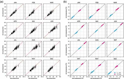
Figure 3(a) shows the validation results for extreme precipitation in terms of the 99% quantile of wet days for all 45 stations and months. In general, the modelled daily precipitation is in good agreement with the observed data. However, a few stations show underestimation in June and August, which is likely related to the challenge of capturing extreme precipitation of convective storms. A further check of the probabilities of wet days (not shown here) indicates a slight underestimation (1–3%). However, the higher observed probabilities are completely within the 90% range of the simulation results for all stations.

The characteristics of the observed daily mean temperature were well reproduced by the weather generator. Figure 3(b) presents the validation results for the simulated minimum and maximum temperatures for each station and month. Besides the good agreement of median values, the temperature modelling is also quite robust. The difference between the 5% and 95% quantiles of the 100 realizations is on average less than 2°C.

Figure 3. Validation results of the weather generator for each month and station. (a) Daily precipitation: the 99% quantile of 43 years of generated precipitation is compared with observed data (43 years). The error bars show the median of 100 realizations with the lower and upper boundaries at the 5% and 95% quantiles. (b) Mean temperature: the maximum and minimum simulated mean temperatures are compared to the corresponding observed data

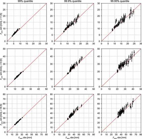
Similarly to the weather generator results, the disaggregation procedure was validated by the comparison of disaggregated and observed data. The hourly data were first aggregated to daily data and then disaggregated back to hourly time steps. While the daily precipitation amount was preserved by the disaggregation method, the hourly intensities differed from the observations. Figure 4 shows the behaviour for extreme precipitation regarding the 99%, 99.9% and 99.95% quantiles of the precipitation series. The quantiles are approximately the 230th, 23th and 12th highest values of the hourly series. The results show a good agreement between the observed and modelled precipitation intensities for durations of 1, 3 and 6 h. As expected, the uncertainty increases for higher quantiles. The slight overestimation for the 99.95% quantile occurs if sampled days for disaggregation have shorter wet spells than the events of the original data. This may also be a result of the limited available hourly data. Like the precipitation amount, the daily mean temperature was preserved by the disaggregation to hourly values. Comparing the simulated and observed minimum and maximum temperatures (hourly time steps), the root mean square error (RMSE) ranges between 0.6–1.7°C (minimum) and 0.5–2.2°C (maximum) for all stations. This is an acceptable range for the application, but can be relevant if the temperature is close to freezing point and triggers the separation of snow and rain events.

Figure 4. Validation results of the disaggregation procedure. The upper tail of the precipitation distribution of 13 years of disaggregated data is compared to observed data. The error bars represent the median and the 5% to 95% uncertainty range from 100 model realizations for each station $\left(n=45\right)$. The columns show the 99%, 99.9% and 99.95% quantiles of the wet hours, while the rows show the precipitation sums of 1, 3 and 6 h duration, respectively

4.2 Runoff modelling and design flood estimation

In the last step of the modelling chain, the generated hourly data were transformed into continuous runoff series by the rainfall–runoff model HQsim. The rainfall–runoff model was calibrated (2001–2007) and validated (2007–2013) against the river gauging data in a classical split-sample approach for all catchments (see Fig. 1). The calibration results of the rainfall–runoff model are shown in Table 2. Besides the NSE, the slightly modified Kling-Gupta efficiency (${\mathrm{K}\mathrm{G}\mathrm{E}}^{\prime }$) according to Kling et al. (2012) was also calculated. The ${\mathrm{K}\mathrm{G}\mathrm{E}}^{\prime }$ is a combined index of the correlation coefficient, bias ratio and variability ratio (Kling et al. 2012). Note, the ${\mathrm{K}\mathrm{G}\mathrm{E}}^{\prime }$ was not used in the calibration procedure. In general, the hydrological model fitted well, with an average NSE of 0.68 and 0.67 (${\mathrm{K}\mathrm{G}\mathrm{E}}^{\prime }$: 0.75 and 0.74) for the calibration and validation periods, respectively.

Table 2. Rainfall–runoff model performance and the estimated discharge of the 100-year flood event by the continuous modelling approach for all catchments. Cal.: calibration; Val.: validation

Gauge	Model performance				Discharge estimate, Q(m^3 s^−1)*
	NSE (-)		KGE (-)		Ensemble estimate (100 × 63 years)
	Cal.	Val.	Cal.	Val.	Median	5% quantile	95% quantile	10 000-year estimate
Au	0.75	0.59	0.80	0.71	261	208	334	264
Hopfreben	0.65	0.53	0.71	0.67	101	80	134	102
Kennelbach	0.73	0.69	0.75	0.71	1900	1481	2439	1945
Mellau	0.76	0.66	0.78	0.75	517	408	679	525
Thal Martinsbrück	0.44	0.58	0.54	0.68	163	129	203	168
Enz	0.75	0.74	0.77	0.72	197	151	248	198
Hoher Steg	0.85	0.80	0.84	0.78	250	199	323	255
Lauterach	0.89	0.86	0.86	0.80	337	265	426	339
Laterns	0.73	0.79	0.73	0.79	134	99	179	135
Bürs	0.64	0.70	0.82	0.83	55	45	72	57
Garsella	0.60	0.60	0.73	0.78	111	87	145	116
Gisingen	0.49	0.46	0.64	0.68	1007	796	1390	1049
Schruns	0.66	0.77	0.77	0.87	92	69	129	94
Unterhochsteg	0.67	0.72	0.75	0.76	156	121	204	159
Lech Tannbrück	0.60	0.59	0.66	0.68	120	85	165	123
Lech	0.72	0.66	0.74	0.75	30	20	41	30

*100-year return period.

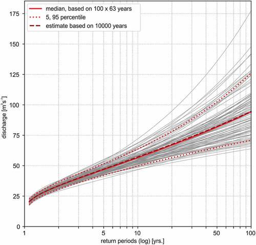
The 100-year flood was estimated by fitting the GEV distribution to the 100 realizations of time series of 63 years’ length. This length is comparable to the longest gauging observations, while in total 6300 years of simulation are enough to compute a robust median value. The 90% uncertainty range based on the sample uncertainty of 63 years was derived from the simulation ensemble. Additionally, the 100-year flood was estimated by fitting the GEV distribution to the entire synthetic series of 10 000 years of generated data. Figure 5 shows the exemplary results of the gauge Schruns, with the individual results of the 100 realizations, the median value, and the 5% and 95% quantiles. The estimates for all catchments are listed in Table 2.

Figure 5. Flood frequency curves for the gauge Schruns derived by the continuous modelling approach. The grey lines indicate the 100 realizations of the modelling procedure with its median value as well as the lower and upper bounds (5% and 95% percentiles). Further, the estimate based on 10 000 years of simulated data is shown

4.3 Comparison of observed and simulated spatial patterns of peak runoff

To ensure the validity of the continuous model chain, several aspects have to be checked. In a first step, the observed and simulated results of the weather generator, the disaggregation procedure and hydrological model were compared at individual sites. The spatial coherence of observed and simulated data of the multi-site CMA approach is assessed by the spatial dependence measure $N_j\left(p\right)$. The comparison of the spatial patterns comprised 14 of the 16 gauging stations, with 42 years of data. Due to the shorter observation length, the gauges Lauterach and Bürs were excluded from the comparison. The value of $N_j\left(p\right)$ was calculated for the observed runoff and 42 years of CMA simulations with 100 realizations. The spatial dependence measure $N_j\left(p\right)$ was analysed for quantile values between 0.9 and 0.998; $p=0.9$ roughly corresponds to 12 events per year and $p=0.998$ refers to a total of 10 events in the 42-year series.

Figure 6 shows the comparison of observed and simulated patterns for three levels of extremeness ($p=0.9,0.99,0.995$). Overall, the spatial dependence measure of observed and simulated data declines for higher levels of extremeness (see Fig. 6(a)–(c)). The mean absolute error between observed and simulated data ranges between 0.05 and 0.08 for all analysed $p$ values (percentage error: 14–26%). The northern catchments (Unterhochsteg and Thal) as well as the gauges in the east (Lech) and south (Schruns) are more independent in comparison to the Bregenzerach, Dornbirnerach and Frutz (Kennelbach, Au, Mellau, Hoher Steg, Enz and Laterns). The stronger dependence can be explained by orographic effects, which occur along the mountain ridges, and predominant weather patterns (see Section 2).

Figure 6. Spatial patterns) $N_j\left(p\right)$ of the observed and simulated peak flows for (a) $p=0.9$, (b) $p=0.99$ and (c) $p=0.995$

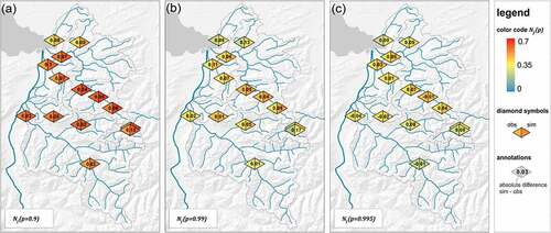
In general, the spatial dependence was reproduced well by the CMA (median of 100 realizations), although the simulations are characterized by slightly higher dependence than the observed values. One reason could be a reduction of the spatial variability by the fitting of the weather generator. Furthermore, the short time series of hourly observed data, as well as the necessary interpolation for stations without sub-daily information for the disaggregation, could have reduced the spatial variability. The possibility to reproduce the spatial dependencies between the gauging stations is a significant advantage of the presented continuous modelling approach compared to the other discussed methods, particularly when it comes to the assessment of flood risk.

5 Comparison and discussion of methods

In the following, the results of the CMA are discussed in comparison to the FFA and DSA approaches. The first part of the comparison covers the peak discharge estimation of a 100-year flood, while the second part presents the variability of runoff volumes within the identified flood events.

5.1 Peak discharge

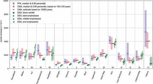
The estimations of 100-year flood peaks are displayed in Figure 7, which includes, besides the continuous modelling approach, the results of the flood frequency analysis of the observed gauging data and of the design storm approach with four different storm types. The confidence intervals are displayed for the FFA and CMA, while the range for each DSA storm type covers the lower to upper pre-event condition scenarios.

The FFA is based on long time series with roughly 60 years of measurements for most gauges (see Table 1). Despite the relatively long observational records, the FFA estimates show a considerable uncertainty range in terms of the sampling uncertainty estimated by the bootstrapping procedure. Due to relatively high precipitation amounts compared to other regions in Austria, the estimated specific discharges of the 100-year flood events are rather high. This outcome is in accordance with findings of the national flood discharge mapping in Austria by Merz et al. (2008).

Figure 7. Peak discharge of the 100-year flood event, derived by the continuous simulation (CMA), by the flood frequency analysis of observed data (FFA), and by the design storm approach with four types of temporal rainfall pattern (DSA). The ${\chi }^2$ goodness-of-fit test suggests that the GEV distribution (FFA) is not fitted adequately for the marked gauges (*)

Most estimates of the continuous simulation are in good agreement with the FFA results; however, in some cases large differences occur. The median values of 13 of the 16 estimates of the 100-year flood event (CMA) are within the FFA confidence interval, whereby the medians of 11 estimates have a relative difference $(100\times \left(\mathrm{C}\mathrm{M}\mathrm{A}-\mathrm{F}\mathrm{F}\mathrm{A}\right)/\mathrm{F}\mathrm{F}\mathrm{A}$) of ≤20% and five estimates are as close as 10% in regard to the FFA median. The absolute discharge values, as well as the percentage errors comparing the CMA results to the FFA, are given in Table 3.

Table 3. Comparison of the modelling results (RP100 discharge) and relative difference in comparison to the flood frequency analysis of the gauging data. The ${\chi }^2$ goodness-of-fit test suggests that the GEV distribution is not fitted adequately for the marked sites (*)

Gauge	RP100 discharge (m^3 s^−1)						relative difference (%)
	FFA	CMA Median	DSA Block	DSA Start	DSA Middle	DSA End	CMAMedian	DSA Block	DSA Start	DSA Middle	DSA End
Au	256*	261	318	356	465	513	2	24	39	82	100
Hopfreben	112	101	81	82	93	92	−10	−28	−27	−17	−18
Kennelbach	1335	1900	1336	1337	1795	1962	42	0	0	34	47
Mellau	443	517	393	424	548	592	17	11	−4	24	34
Thal-Martinsbrück	226	163	112	112	118	113	−28	−50	−50	−48	−50
Enz	223	197	193	189	214	215	−12	−14	−15	−4	−4
Hoher Steg	233	250	201	195	222	228	7	−14	−16	−5	−2
Lauterach	296*	337	270	268	306	312	14	−9	−9	3	5
Laterns	180	134	23	23	25	25	−26	−87	−87	−86	−86
Bürs	69*	55	39	39	42	43	−20	−43	−43	−39	−38
Garsella	106	111	81	82	94	96	5	−23	−23	−11	−10
Gisingen	708	1007	445	586	701	696	42	−37	−17	−1	−2
Schruns	100	92	58	60	68	68	−8	−42	−40	−32	−32
Unterhochsteg	189	156	204	206	223	233	−17	8	9	18	24
Lech Tannbrück	145	120	82	76	91	96	−17	−44	−48	−37	−34
Lech	55	30	24	23	26	28	−45	−55	−58	−53	−49

The CMA estimates for the gauge Lech are lower than the FFA results. In contrast, the two largest catchments (the Bregenzerache River at Kennelbach and the Ill River at Gisingen) show an approximately 40% higher estimate in comparison to the FFA. Rogger et al. (2012b) identified step changes in the frequency curve due to the exceedence of storage thresholds of the hydrological system. This could be a possible reason for larger CMA estimates in comparison to the traditional FFA. However, this effect could not be identified for the two catchments. Furthermore, the slight overestimation in the disaggregation procedure may influence the results towards higher estimates. Another reason could be the influence of hydropower reservoirs cutting peak discharges, especially for the upper Ill catchment. This effect is not considered in the hydrological model set-up, but is contained in the discharge records.

In comparison to the CMA results, the DSA results are systematically lower compared to the flood frequency approach. This may be a result of the chosen critical rainfall duration and areal reduction factor. In particular, the results of the block rainfall show low discharge estimates, with only six of the 16 estimates inside the FFA confidence interval. In contrast, the end-emphasized storms frequently result in the highest DSA estimates. This indicates that the flood events of the catchments are triggered mostly by the peak rainfall intensity, which is lowest for block rainfall. Additionally, the saturation of the hydrological storages is highest for an end-emphasized storm when the peak intensity is reached. The DSA method seems to be inappropriate for the gauge Laterns, which may be the result of an inappropriate IDF curve or inappropriate critical duration for the small catchment. For most DSA estimates, the choice of catchment state and storm type alters the peak discharge considerably (see Fig. 7). In contrast to the CMA method, where event pre-conditions and both temporal and spatial patterns of precipitation are modelled implicitly, each of the DSA realizations is based on a rather subjective a priori decision.

5.2 Flood event runoff volume

Besides the peak discharge, the hydrographs of simulated flood events and their runoff volumes are analysed. Without the application of multi-variate models, the FFA gives no direct insights into runoff volume corresponding to the estimated peak discharge. In contrast, the result of the CMA is a continuous runoff series, from which all related event characteristics can be directly derived. The hydrographs for all events reaching the peak flow of a $T$-year flood (±5% of the ensemble median estimate) are extracted from the runoff series.

Figure 8 summarizes the results for the event volume for two example catchments. As expected, the runoff volume generally rises alongside the discharge peaks with higher return periods. Nonetheless, the highest event volumes do not necessarily correspond to the largest peak flows. This can be explained by longer event durations, as depicted, for example, in Figure 8(d) and (f). As shown by Gaál et al. (2015) and Szolgay et al. (2016), mountain catchments in particular are characterized by a weak dependence between flood peaks and volumes because of their diversity of flood types (synoptic, snowmelt and flash floods).

Figure 8. Comparison of peak discharge, corresponding event volume and duration of T-year flood events for (a, c, e) Mellau at Bregenzerach and (b, d, f) Lauterach at Dornbirner Ache. The range (shaded in red) shows the variability of the CMA results in terms of 5% and 95% quantiles of all identified events. The FFA is performed on peak discharge only

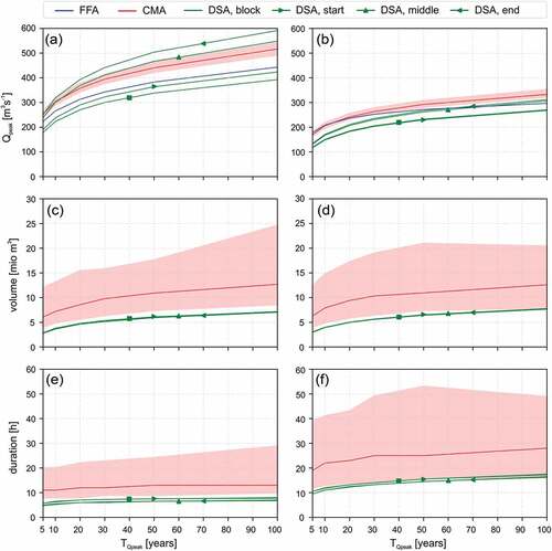
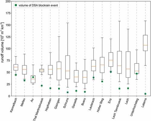
Analysis of the CMA hydrographs identifies a large variability of event volumes for roughly the same peak discharges (±5%). This variability results from different spatio-temporal precipitation and soil moisture patterns inherent in the CMA approach. In contrast, the individual hydrographs of the DSA events result in a single estimate of runoff volume, with no further information about possible variability. Generally, the DSA leads to lower event volumes. As the different storm types are based on an identical precipitation amount, only the precipitation distribution during the events differs, with marginal effects on the total runoff volume. Figure 9 shows the variability of runoff volume for the identified 100-year CMA events and the DSA block rainfall type (standardized by the catchment size). The DSA results do not fully account for the variability of possible flood events, which can lead to considerably lower possible runoff volumes, as shown by the comparison to the CMA approach. The findings are in accordance with Grimaldi et al. (2013), who showed that the use of the design storm approach may lead to an underestimation of flood volumes in comparison to a fully continuous model simulation. This is an important outcome, as the potential damage due to flooding is influenced by both the flood peak and the runoff volume during an event (Dung et al. 2015, Lamb et al. 2016).

Figure 9. Box plots of runoff volume (m³ km⁻²) corresponding to the peak discharge (±5%) of a 100-year flood event for the CMA and the DSA block rain type. The volume is standardized by the catchment area

5.3 Uncertainties and limitations

The ensemble of the CMA members with time series length comparable to observations represents the sampling uncertainty in this approach. By the generation of long time series (e.g. 10 000 years) and fitting the flood frequency distribution to the entire sample, the sampling uncertainty can be reduced in comparison to the FFA on observed data (Rogger et al. 2012b). In the CMA, a plethora of unobserved but plausible weather situations can be generated and consistently combined with various catchment conditions. This combination can result in estimating potential but so far unobserved flood situations. However, the true variability range remains unknown. In the continuous modelling approach, further assumptions about critical storm durations or pre-event catchment states can be avoided (Grimaldi and Petroselli 2015). An obvious disadvantage of the CMA method is its complexity, which accounts especially for spatially distributed approaches (Breinl 2016). As a consequence of the application of multiple models, the degrees of freedom increase, with additional sources of structural and parameter uncertainties (Arnaud et al. 2017). In this study, these include for example uncertainties of the hydrological model (Montanari 2011), the choice of the objective function (Moussa and Chahinian 2009), the uncertainty within the meteorological input data (Arnaud et al. 2011) and the uncertainty introduced by the spatial interpolation of meteorological variables (Wagner et al. 2012).

Not only the complex model chain of the CMA, but also the FFA and DSA are subject to uncertainties. Besides the debatable assumption of identity of rainfall and runoff return period (Viglione et al. 2009), the IDF curves themselves are uncertain, for example due to the length of meteorological time series, subsequent spatial interpolation procedures, or more generally the applied estimation methods (Mélèse et al. 2018). The choice of pre-event catchment state is another major source of uncertainty, which needs to be managed by the analyst (Boughton and Droop 2003, Grimaldi and Petroselli 2015). Additionally, independent of the method to transform event precipitation into discharge, some sort of calibration and validation based on streamflow samples is also needed for DSA (Rogger et al. 2012a). In this study, the identical hydrological model was applied for the CMA and DSA, including all related sources of uncertainty. On the one hand, the use of the same model ensures an identical hydrological response to the input data, while on the other hand the results are not completely independent, which weakens the significance of identical results.

Besides the length of available observation data, the FFA on runoff observations is also subject to additional uncertainties, such as the choice of the distribution function and the fitting procedure. This is also true when the FFA is applied to simulated data. However, much longer time series can be generated. The measurement uncertainty for meteorological and hydrological data is inherent in all three methods. In particular, discharge observations are usually obtained by transformation of measured water levels using rating curves, which change over time (Di Baldassarre and Montanari 2009). Nevertheless, if only peak flow is of interest and sufficiently long time series of appropriate quality are available at the site, the FFA has its advantages, as it is easy to apply in a widely standardized procedure (e.g. Robson and Reed 1999).

In this study, different sources of uncertainties were accounted for in the applied approaches. This did not allow for straightforward comparison of their uncertainty ranges. A more comprehensive uncertainty assessment, e.g. sampling uncertainty of the weather generator due to short meteorological observation series, was difficult due to computational constraints and complexity of the approaches (Rogger et al. 2012a, Grimaldi et al. 2012b). However, the comparison of the results itself can help to identify uncertainties in model inputs and assumptions and will, in the case of good agreement, increase the trustworthiness of the results (Gutknecht et al. 2006).

The traditional univariate FFA needs to be extended to a multi-variate analysis in order to estimate further flood characteristics such as flood event volume (Mediero et al. 2010). Serinaldi and Grimaldi (2011) overcame the limitation by linking the flood volume and duration to a fixed return period, based on different distribution functions. The concept was further extended to a fully joint description of discharge and volume by means of a copula approach by Brunner et al. (2017). In any case, multi-variate models need to be applied to the FFA, whereas event hydrographs are directly derived by the DSA and CMA approaches. In the case of DSA, the same limitations do apply for the estimate of volume as for peak discharges (e.g. assumption of identity of return periods, choice of pre-event conditions). Furthermore, the large variability of runoff volume for a given return period is difficult to capture, while different underlying flood generation processes are taken into account implicitly for the CMA approach. In the case of DSA, this may also result in a possible underestimation of runoff volume for flood events (Grimaldi et al. 2012b, 2013).

All three applied methods rely on the assumption of stationarity. The assumption is undermined not only by water management interventions, but also by land-cover dynamics and climate change (Milly et al. 2008). The traditional FFA can be extended to non-stationary flood frequency analysis, but it remains highly uncertain in the case of limited observational data (Serinaldi and Kilsby 2017). Inclusion of physically-based processes in the continuous modelling approach allows one to incorporate non-stationarity in design flood estimations (Breinl 2016, Lamb et al. 2016). This may include trends in meteorological input variables to address climate change (Raff et al. 2009, Hundecha and Merz 2012, Madsen et al. 2014), land-use development scenarios (Holzmann et al. 2010, Gupta et al. 2015, Rogger et al. 2017), or the co-evolution of multiple relevant drivers (Elshafei et al. 2014).

6 Conclusion

In this study, a fully continuous modelling approach to estimate low-frequency flood events (e.g. 100-year flood) was implemented in combination with a disaggregation procedure to hourly time scale and applied in 16 mountainous catchments in Austria. It was demonstrated that the CMA leads to plausible results, which are often comparable to the flood frequency analysis. The median values of 13 of the 16 peak flow estimates are inside the 5–95% confidence interval of the FFA. In comparison, the design storm approach more often resulted in an underestimation of the FFA peak flows, depending on the assumed storm type. At some stations, there were larger differences between the applied methods. However, it is hardly possible to identify the “correct” estimation, as all methods are based on the extrapolation of observed patterns in one way or another.

The results indicate that single-event hydrographs of the DSA method can lead to a considerable underestimation of event volumes. In contrast, the CMA gives insights into the variability of runoff volumes, since it includes the variability in the pre-event catchment states, as well as the temporal and spatial rainfall patterns. By forcing the hydrological model with spatially coherent, generated and disaggregated meteorological input data, the spatial dependence patterns within the study area can be well reproduced by the CMA. Therefore, not only peak estimates at single gauges, but trans-basin flood events across the study area can be derived by the CMA on an hourly time scale. The spatially coherent modelling of flood events across multiple catchments is of special importance for large-scale flood risk estimation (Falter et al. 2015, Schneeberger et al. 2017).

Acknowledgments

We would like to thank all the institutions that provided data, the Zentralanstalt für Meteorologie and Geodynamik (ZAMG), the Deutscher Wetterdienst (DWD), and particularly the Hydrographischer Dienst Vorarlberg. The simulations were conducted using the Vienna Scientific Cluster (VSC). Finally, we want to thank Korbinan Breinl and the two anonymous reviewers for their valuable comments and suggestions.

Disclosure statement

No potential conflict of interest was reported by the authors.

Additional information

Funding

This work results from the research project InsuRE II, funded by the Austrian Research Promotion Agency (FFG), within the scope of the program COMET and the project HiFlow-CMA [KR15AC8K12522] funded by the Austrian Climate and Energy Fund (ACRP 8th call).

References

- Achleitner, S., et al., 2012. Analysing the operational performance of the hydrological models in an alpine flood forecasting system. Journal of Hydrology, 412-413, 90–100. doi:10.1016/j.jhydrol.2011.07.047
- Achleitner, S., Rinderer, M., and Kirnbauer, R., 2009. Hydrological modeling in alpine catchments. Sensing the critical parameters towards an efficient model calibration. Water Science and Technology: a Journal of the International Association on Water Pollution Research, 60 (6), 1507–1514. doi:10.2166/wst.2009.488
- Andrieu, C., et al., 2003. An introduction to MCMC for machine learning. Machine Learning, 50 (1/2), 5–43. doi:10.1023/A:1020281327116
- Arnaud, P., et al., 2011. Sensitivity of hydrological models to uncertainty in rainfall input. Hydrological Sciences Journal, 56 (3), 397–410. doi:10.1080/02626667.2011.563742
- Arnaud, P., Cantet, P., and Odry, J., 2017. Uncertainties of flood frequency estimation approaches based on continuous simulation using data resampling. Journal of Hydrology, 554, 360–369. doi:10.1016/j.jhydrol.2017.09.011
- Bavay, M. and Egger, T., 2014. MeteoIO 2.4.2: a preprocessing library for meteorological data. Geoscientific Model Development, 7 (6), 3135–3151. doi:10.5194/gmd-7-3135-2014
- Blazkova, S. and Beven, K., 1997. Flood frequency prediction for data limited catchments in the Czech Republic using a stochastic rainfall model and TOPMODEL. Journal of Hydrology, 195 (1–4), 256–278. doi:10.1016/S0022-1694(96)03238-6
- Blazkova, S. and Beven, K., 2004. Flood frequency estimation by continuous simulation of subcatchment rainfalls and discharges with the aim of improving dam safety assessment in a large basin in the Czech Republic. Journal of Hydrology, 292 (1–4), 153–172. doi:10.1016/j.jhydrol.2003.12.025
- Blöschl, G., ed., 2009. Hochwässer - Bemessung, Risikoanalyse und Vorhersage. ÖWAV- Seminar, Bundesamtsgebäude Wien, 26. Mai 2009. Wien: Techn. Univ. Wien, Inst. f. Wasserbau und Ingenieurhydrologie.
- Blöschl, G., et al., eds. 2013. Runoff prediction in ungauged basins. Synthesis across processes, places and scales. Cambridge: Cambridge University Press.
- BMLFUW, 2007. Hydrologischer Atlas Österreich. 3rd ed. Wien: Bundesministerium für Land- und Forstwirtschaft, Umwelt und Wasserwirtschaft (BMLFUW).
- BMLFUW, ed., 2011. Verfahren zur Abschätzung von Hochwasserkennwerten. Leitfaden. Wien: Bundesministerium für Land- und Forstwirtschaft, Umwelt und Wasserwirtschaft (BMLFUW).
- Boughton, W. and Droop, O., 2003. Continuous simulation for design flood estimation? A review. Environmental Modelling & Software, 18 (4), 309–318. doi:10.1016/S1364-8152(03)00004-5
- Breinl, K., 2016. Driving a lumped hydrological model with precipitation output from weather generators of different complexity. Hydrological Sciences Journal, 61 (8), 1395–1414. doi:10.1080/02626667.2015.1036755
- Breinl, K., et al., 2017. A joint modelling framework for daily extremes of river discharge and precipitation in urban areas. Journal of Flood Risk Management, 10 (1), 97–114. doi:10.1111/jfr3.12150
- Brunner, M.I., et al., 2017. Flood type specific construction of synthetic design hydrographs. Water Resources Research, 53 (2), 1390–1406. doi:10.1002/2016WR019535
- Buishand, T.A. and Brandsma, T., 2001. Multisite simulation of daily precipitation and temperature in the Rhine Basin by nearest-neighbor resampling. Water Resources Research, 11 (37), 2761–2776. doi:10.1029/2001WR000291
- Burn, D.H., 2003. The use of resampling for estimating confidence intervals for single site and pooled frequency analysis/Utilisation d’un rééchantillonnage pour l’estimation des intervalles de confiance lors d’analyses fréquentielles mono et multi-site. Hydrological Sciences Journal, 48 (1), 25–38. doi:10.1623/hysj.48.1.25.43485
- Coles, S., 2001. An introduction to statistical modeling of extreme values. 4th. London: Springer.
- Dastorani, M., et al., 2013. River instantaneous peak flow estimation using daily flow data and machine-learning-based models. Journal of Hydroinformatics, 15, 1089–1098. doi:10.2166/hydro.2013.245
- Di Baldassarre, G. and Montanari, A., 2009. Uncertainty in river discharge observations. A quantitative analysis. Hydrology and Earth System Sciences, 13 (6), 913–921. doi:10.5194/hess-13-913-2009
- Dobler, C. and Pappenberger, F., 2013. Global sensitivity analyses for a complex hydrological model applied in an Alpine watershed. Hydrological Processes, 27 (26), 3922–3940. doi:10.1002/hyp.9520
- Dung, N.V., et al., 2015. Handling uncertainty in bivariate quantile estimation – an application to flood hazard analysis in the Mekong Delta. Journal of Hydrology, 527, 704–717. doi:10.1016/j.jhydrol.2015.05.033
- DVWK, ed., 1984. DVWK 113/1984. Arbeitsanleitung zur Anwendung von Niederschlag-Abfluß-Modellen in kleinen Einzugsgebieten. Hamburg: Deutscher Verband für Wasserwirtschaft und Kulturbau (DVWK).
- DWA, ed., 2012. Ermittlung von Hochwasserwahrscheinlichkeiten. Merkblatt DWA-M 552. Hennef: Deutsche Vereinigung für Wasserwirtschaft, Abwasser und Abfall (DWA).
- Elshafei, Y., et al., 2014. A prototype framework for models of socio-hydrology. Identification of key feedback loops and parameterisation approach. Hydrology and Earth System Sciences, 18 (6), 2141–2166. doi:10.5194/hess-18-2141-2014
- European Union (EU), 2007. European Union on the assessment and management of flood risks. Directive 2007/60/EC of the European Parliament and the Council. Official Journal of the European Union L288/27. Available from: https://eur-lex.europa.eu/legal-content/EN/TXT/PDF/?uri=CELEX:32007L0060&from=EN.
- Falter, D., et al., 2015. Spatially coherent flood risk assessment based on long-term continuous simulation with a coupled model chain. Journal of Hydrology, 524, 182–193. doi:10.1016/j.jhydrol.2015.02.021
- Förster, K., et al., 2016. An open-source MEteoroLOgical observation time series DISaggregation Tool (MELODIST v0.1.1). Geoscientific Model Development, 9 (7), 2315–2333. doi:10.5194/gmd-9-2315-2016
- Gaál, L., et al., 2015. Dependence between flood peaks and volumes. A case study on climate and hydrological controls. Hydrological Sciences Journal, 60 (6), 968–984. doi:10.1080/02626667.2014.951361
- Goovaerts, P., 2000. Geostatistical approaches for incorporating elevation into the spatial interpolation of rainfall. Journal of Hydrology, 228 (1–2), 113–129. doi:10.1016/S0022-1694(00)00144-X
- Grimaldi, S., et al., 2012a. Time of concentration. A paradox in modern hydrology. Hydrological Sciences Journal, 57 (2), 217–228. doi:10.1080/02626667.2011.644244
- Grimaldi, S., et al., 2013. Flood mapping in ungauged basins using fully continuous hydrologic–hydraulic modeling. Journal of Hydrology, 487, 39–47. doi:10.1016/j.jhydrol.2013.02.023
- Grimaldi, S. and Petroselli, A., 2015. Do we still need the rational formula? An alternative empirical procedure for peak discharge estimation in small and ungauged basins. Hydrological Sciences Journal, 60 (1), 67–77. doi:10.1080/02626667.2014.880546
- Grimaldi, S., Petroselli, A., and Serinaldi, F., 2012b. Design hydrograph estimation in small and ungauged watersheds. Continuous simulation method versus event-based approach. Hydrological Processes, 26 (20), 3124–3134. doi:10.1002/hyp.8384
- Güntner, A., et al., 2001. Cascade-based disaggregation of continuous rainfall time series: the influence of climate. Hydrology and Earth System Sciences, 5 (2), 145–164. doi:10.5194/hess-5-145-2001
- Gupta, S.C., et al., 2015. Climate and agricultural land use change impacts on streamflow in the upper midwestern United States. Water Resources Research, 51 (7), 5301–5317. doi:10.1002/2015WR017323
- Gutknecht, D., et al., 2006. Ein “Mehr-Standbeine”-Ansatz zur Ermittlung von Bemessungshochwässern kleiner Auftretenswahrscheinlichkeit. Österreichische Wasser- und Abfallwirtschaft, 58 (3–4), 44–50. doi:10.1007/BF03165683
- Haberlandt, U., et al. 2011. Rainfall generators for application in flood studies. In: A.H. Schumann, ed. Flood risk assessment and management. Dordrecht: Springer Netherlands, 117–147. doi:10.1007/978-90-481-9917-4_7
- Haberlandt, U. and Radtke, I., 2014. Hydrological model calibration for derived flood frequency analysis using stochastic rainfall and probability distributions of peak flows. Hydrology and Earth System Sciences, 18 (1), 353–365. doi:10.5194/hess-18-353-2014
- Holzmann, H., et al., 2010. Auswirkungen möglicher Klimaänderungen auf Hochwasser und Wasserhaushaltskomponenten ausgewählter Einzugsgebiete in Österreich. Österreichische Wasser- und Abfallwirtschaft, 62 (1–2), 7–14. doi:10.1007/s00506-009-0154-9
- Hosking, J.R.M. and Wallis, J.R., 1997. Regional frequency analysis. An approach based on L-moments. Cambridge: Cambridge University Press.
- Hundecha, Y. and Merz, B., 2012. Exploring the relationship between changes in climate and floods using a model-based analysis. Water Resources Research, 48 (4). doi:10.1029/2011WR010527
- Hundecha, Y., Pahlow, M., and Schumann, A., 2009. Modeling of daily precipitation at multiple locations using a mixture of distributions to characterize the extremes. Water Resources Research, (45. doi:10.1029/2008WR007453
- Keef, C., Tawn, J., and Svensson, C., 2009. Spatial risk assessment for extreme river flows. Journal of the Royal Statistical Society: Series C (Applied Statistics), 58 (5), 601–618. doi:10.1111/j.1467-9876.2009.00672.x
- Kleindienst, H., 1996. Erweiterung und Erprobung eines anwendungsorientierten hydrologischen Modells zur Gangliniensimulation in kleinen Wildbacheinzugsgebie. Diplomarbeit.
- Kling, H., Fuchs, M., and Paulin, M., 2012. Runoff conditions in the upper Danube basin under an ensemble of climate change scenarios. Journal of Hydrology, 424-425, 264–277. doi:10.1016/j.jhydrol.2012.01.011
- Kossieris, P., et al. 2016. A rainfall disaggregation scheme for sub-hourly time scales. Coupling a bartlett-lewis based model with adjusting procedures. Journal of Hydrology. doi:10.1016/j.jhydrol.2016.07.015
- Koutsoyiannis, D., Onof, C., and Wheater, H.S., 2003. Multivariate rainfall disaggregation at a fine timescale. Water Resources Research, 39, 7. doi:10.1029/2002WR001600
- Kyselý, J., 2008. A cautionary note on the use of nonparametric bootstrap for estimating uncertainties in extreme-value models. Journal of Applied Meteorology and Climatology, 47 (12), 3236–3251. doi:10.1175/2008JAMC1763.1
- Lall, U. and Sharma, A., 1996. A nearest neighbor bootstrap for resampling hydrologic time series. Water Resources Research, 32 (3), 679–693. doi:10.1029/95WR02966
- Lamb, R., et al., 2016. Have applications of continuous rainfall–runoff simulation realized the vision for process-based flood frequency analysis? Hydrological Processes, 30 (14), 2463–2481. doi:10.1002/hyp.10882
- Leander, R. and Buishand, T.A., 2009. A daily weather generator based on a two-stage resampling algorithm. Journal of Hydrology, 374 (3–4), 185–195. doi:10.1016/j.jhydrol.2009.06.010
- Madsen, H., et al., 2014. Review of trend analysis and climate change projections of extreme precipitation and floods in Europe. Journal of Hydrology, 519, 3634–3650. doi:10.1016/j.jhydrol.2014.11.003
- Maniak, U., 2010. Hydrologie und Wasserwirtschaft. Eine Einführung für Ingenieure. Berlin, Heidelberg: Springer-Verlag.
- Mediero, L., Jiménez-Álvarez, A., and Garrote, L., 2010. Design flood hydrographs from the relationship between flood peak and volume. Hydrology and Earth System Sciences, 14 (12), 2495–2505. doi:10.5194/hess-14-2495-2010
- Mélèse, V., Blanchet, J., and Molinié, G., 2018. Uncertainty estimation of Intensity–Duration–Frequency relationships. A regional analysis. Journal of Hydrology, 558, 579–591. doi:10.1016/j.jhydrol.2017.07.054
- Merz, R., Blöschl, G., and Humer, G., 2008. National flood discharge mapping in Austria. Natural Hazards, 46 (1), 53–72. doi:10.1007/s11069-007-9181-7
- Milly, P.C.D., et al., 2008. Climate change. Stationarity is dead. Whither water management? Science (New York, N.Y.), 319 (5863), 573–574. doi:10.1126/science.1151915
- Montanari, A., 2011. Uncertainty of hydrological predictions. In: P. Wilderer, ed. Treatise on water science. Oxford: Academic Press, 459–478.
- Moussa, R. and Chahinian, N., 2009. Comparison of different multi-objective calibration criteria using a conceptual rainfall–runoff model of flood events. Hydrology and Earth System Sciences, 13 (4), 519–535. doi:10.5194/hess-13-519-2009
- Müller, H. and Haberlandt, U., 2018. Temporal rainfall disaggregation using a multiplicative cascade model for spatial application in urban hydrology. Journal of Hydrology. 556, 847–864. doi:10.1016/j.jhydrol.2016.01.031
- Nash, J.E. and Sutcliffe, J.V., 1970. River flow forecasting through conceptual models part I — A discussion of principles. Journal of Hydrology, 10 (3), 282–290. doi:10.1016/0022-1694(70)90255-6
- Nowak, K., et al., 2010. A nonparametric stochastic approach for multisite disaggregation of annual to daily streamflow. Water Resources Research, 46 (8). doi:10.1029/2009WR008530
- Olsson, J., 1998. Evaluation of a scaling cascade model for temporal rainfall disaggregation. Hydrology and Earth System Sciences, (2), 19–30. doi:10.5194/hess-2-19-1998
- Plouffe, C.C.F., Robertson, C., and Chandrapala, L., 2015. Comparing interpolation techniques for monthly rainfall mapping using multiple evaluation criteria and auxiliary data sources: A case study of Sri Lanka. Environmental Modelling & Software, 67, 57–71. doi:10.1016/j.envsoft.2015.01.011
- Pui, A., et al., 2012. A comparison of alternatives for daily to sub-daily rainfall disaggregation. Journal of Hydrology, 470-471, 138–157. doi:10.1016/j.jhydrol.2012.08.041
- Raff, D.A., Pruitt, T., and Brekke, L.D., 2009. A framework for assessing flood frequency based on climate projection information. Hydrology and Earth System Sciences Discussions, 6 (2), 2005–2040. doi:10.5194/hessd-6-2005-2009
- Rickenmann, D., 1996. Fliessgeschwindigkeit in Wildbächen und Gebirgsflüssen. Wasser Energie Luft, 88 (11/12), 298–304.
- Robson, A. and Reed, D., 1999. Statistical procedures for flood frequency estimation. Wallingford: Institute of Hydrology.
- Rogger, M., et al., 2012a. Runoff models and flood frequency statistics for design flood estimation in Austria? Do they tell a consistent story? Journal of Hydrology, 456-457, 30–43. doi:10.1016/j.jhydrol.2012.05.068
- Rogger, M., et al., 2012b. Step changes in the flood frequency curve. Process controls. Water Resources Research, 48 (5), 147. doi:10.1029/2011WR011187
- Rogger, M., et al., 2017. Land use change impacts on floods at the catchment scale. Challenges and opportunities for future research. Water Resources Research, 53 (7), 5209–5219. doi:10.1002/2017WR020723
- Schneeberger, K., et al. 2017. A probabilistic framework for risk analysis of widespread flood events. A proof-of-concept study. Risk Analysis. doi:10.1111/risa.12863
- Schneeberger, K., Rössler, O., and Weingartner, R., 2018. Spatial patterns of frequent floods in Switzerland. Hydrological Sciences Journal, 63 (6), 895–908. doi:10.1080/02626667.2018.1450505
- Schneeberger, K. and Steinberger, T., 2018. Generation of spatially heterogeneous flood events in an alpine region—Adaptation and application of a multivariate modelling procedure. Hydrology, 5 (1), 5. doi:10.3390/hydrology5010005
- Senfter, S., et al. 2009. Flood Forecasting for the River Inn. In: E. Veulliet, S. Johann, and H. Weck-Hannemann, eds. Sustainable natural hazard management in alpine environments. Berlin, Heidelberg: Springer Berlin Heidelberg, 35–67. doi:10.1007/978-3-642-03229-5_2
- Serinaldi, F. and Grimaldi, S., 2011. Synthetic design hydrographs based on distribution functions with finite support. Journal of Hydrologic Engineering, 16 (5), 434–446. doi:10.1061/(ASCE)HE.1943-5584.0000339
- Serinaldi, F. and Kilsby, C.G., 2017. A blueprint for full collective flood risk estimation. Demonstration for European river flooding. Risk Analysis: an Official Publication of the Society for Risk Analysis, 37 (10), 1958–1976. doi:10.1111/risa.12747
- Sharma, A. and Srikanthan, S., 2006. Continuous rainfall simulation: a nonparametric alternative. In: Hydrology & water resources symposium: past, present and future 2006. Sandy Bay: Conference Design, 86–91.
- Sivapalan, M., et al., 2005. Linking flood frequency to long-term water balance. Incorporating effects of seasonality. Water Resources Research, 41 (6), 1065. doi:10.1029/2004WR003439
- Szolgay, J., et al., 2016. A regional comparative analysis of empirical and theoretical flood peak-volume relationships. Journal of Hydrology and Hydromechanics, 64 (4), 367–381. doi:10.1515/johh-2016-0042
- Viglione, A. and Blöschl, G., 2009. On the role of storm duration in the mapping of rainfall to flood return periods. Hydrology and Earth System Sciences, 13 (2), 205–216. doi:10.5194/hess-13-205-2009
- Viglione, A., Merz, R., and Blöschl, G., 2009. On the role of the runoff coefficient in the mapping of rainfall to flood return periods. Hydrology and Earth System Sciences Discussions, 6 (1), 627–665. doi:10.5194/hessd-6-627-2009
- Viviroli, D., et al., 2009. Continuous simulation for flood estimation in ungauged mesoscale catchments of Switzerland – part II. Parameter regionalisation and flood estimation results. Journal of Hydrology, 377 (1–2), 208–225. doi:10.1016/j.jhydrol.2009.08.022
- Vrac, M. and Naveau, P., 2007. Stochastic downscaling of precipitation: from dry events to heavy rainfalls. Water Resources Research, 43, 7. doi:10.1029/2006WR005308
- Wagner, P.D., et al., 2012. Comparison and evaluation of spatial interpolation schemes for daily rainfall in data scarce regions. Journal of Hydrology, 464-465, 388–400. doi:10.1016/j.jhydrol.2012.07.026
- Weilguni, V., 2009. Bemessungsniederschläge in Österreich. In: G. Blöschl, ed. Hochwässer - Bemessung, Risikoanalyse und Vorhersage. ÖWAV- Seminar, Bundesamtsgebäude Wien, 26. Mai 2009. Wien: Techn. Univ. Wien, Inst. f. Wasserbau und Ingenieurhydrologie, 71–84.
- Westra, S., et al., 2013. A conditional disaggregation algorithm for generating fine time-scale rainfall data in a warmer climate. Journal of Hydrology, 479, 86–99. doi:10.1016/j.jhydrol.2012.11.033