Propagation of uncertainties in interpolated rainfields to runoff errors

ABSTRACT

Conditional daily rainfields were generated using collocated raingauge radar data by a kriging interpolation method, and disaggregated into hourly rainfields using variants of the method of fragments. A geographic information system (GIS)-based distributed rainfall–runoff model was used to convert the hourly rainfields into hydrographs. Using the complete radar rainfall as input, the rainfall–runoff model was calibrated based on storm events taken from nested catchments. Performance statistics were estimated by comparing the observed and the complete radar rainfall simulated hydrographs. Degradation in the hydrograph performance statistics by the simulated hourly rainfields was used to identify runoff error propagation. Uncertainty in daily rainfall amounts alone caused higher errors in runoff (depth, peak, and time to peak) than those caused by uncertainties in the hourly proportions alone. However, the degradation, which reduced with runoff depth, caused by the combined uncertainties was not significantly different from that caused by the uncertainty of amounts alone.

KEYWORDS:

• rainfield
• disaggregation
• conditional simulation
• uncertainty
• runoff errors
• radar rainfall

Editor R. Woods Associate editor E. Volpi

1 Introduction

It is well established in the literature that spatial and temporal rainfall variability is paramount for better assessing the hydrological response of a catchment (e.g. Segond et al. 2007, Zoccatelli et al. 2015), and that it constitutes a major source of hydrological uncertainty. There have been significant inroads on this subject matter, including the use of radar to measure rainfall. Rainfall radar has improved our understanding of the spatial and temporal variability, but has its own shortcomings (e.g. beam blocking and ground clutter sources of errors), and should be used in combination with raingauge network data (e.g. Cole and Moore 2009). Berndt et al. (2014) investigated merging of radar and raingauge data using different geostatistical interpolation techniques. Using different high resolutions and raingauge densities, conditional merging was their preferred technique. Also, radar rainfall is not widely available, and has short record length, of less than 10 years in many regions of the world. However, point daily rainfall measurements of over 100 years in record length are very common worldwide, and there are also a few pluviometers measuring rainfall by the minute. In general, the gauge network density is not sufficient to capture the spatial variability of rainfall. Averaging rainfall over the catchment, particularly using a single raingauge, leads to inaccuracies in the generated hydrograph, which in turn affect the calibrated parameters of a rainfall–runoff model (e.g. Shah et al. 1996).

A typical approach to examining the influence of spatial rainfall is through the use of different levels of rainfall complexity involving radar, and the combination of radar and raingauge network data, in a rainfall–runoff model (e.g. Cole and Moore 2009). At the catchment scale, the influence of spatial variability of runoff could depend on several factors, including the initial moisture conditions, catchment attributes and the runoff generation mechanism (e.g. Merz and Blöschl 2003, Emmanuel et al. 2015). As a result, there are mixed results in the literature. Some conclude that the effects of spatially variable rainfall could be obscured by the averaging effects of runoff routing, while others have established that omitting the spatial variability could result in considerable loss of model efficiency (e.g. Zoccatelli et al. 2010, Tarolli et al. 2013, Emmanuel et al. 2015).

Many regions around the world are devoid of radar rainfall measurements and modellers resort to interpolation of the limited gauged data. However, interpolation results are affected by the raingauge network density, and complex topography compounds the problem. Simple deterministic interpolation methods include Thiessen polygon, inverse distance weighting (IDW), and polynomial and spline interpolation. Different forms of kriging (simple, ordinary, universal and external drift) based on correlogram functions are considered more advanced (e.g. Velasco-Forero et al. 2009). Cross-validation methods are usually used to evaluate the performance of the interpolation methods (e.g. Buytaert et al. 2006). Only a few researchers have used simulated streamflow, at the daily time scale though, to evaluate rainfall interpolation methods (Haberlandt and Kite 1998).

There is a limited number of studies looking into the propagation of spatio-temporal rainfall errors to simulated runoff. Sharif et al. (2002) used a generated radar rainfield of one storm event and distributed hydrological simulations to analyse the propagation of errors from rainfall to runoff. They concluded that the magnitude of errors in runoff (volume and peak) was nearly double that of rainfall volume errors for a 21.2-km² catchment, runoff errors amplifying as the total rainfall volume became smaller. Olsson (2006) considered five rainfall sources and used one as the true source, its associated runoff generated by a rainfall–runoff model also considered the true runoff. He observed discharge bias of up to 79% for catchments ranging between 134 and 2133 km² using a 1-day simulation time scale.

In the literature, temporal disaggregation of daily rainfall to fine time scales is limited to point time series (Glasbey et al. 1995, Cowpertwait et al. 1996, Gyasi-Agyei 2005, 2011). However, simultaneous disaggregation of multi-site point daily rainfall time series, taking into account a form of spatial correlation, has been done (e.g. Koutsoyiannis et al. 2003, Dominguez-Mora et al. 2014). Spatial disaggregation is normally associated with cases where rainfield data of a bigger spatial scale are regenerated into smaller sized grids (e.g. Gagnon et al. 2002).

Approaches based on the method of fragments (MOF) have been used for disaggregating daily rainfall to fine time scales (e.g. Gyasi-Agyei 2012, Pui et al. 2012, Westra et al. 2012, Li et al. 2018). For these approaches, sub-daily fragment vectors, which are ratios of the fine time scale values to the daily ones, are sampled from a pool of at-site records with different sampling methodologies.

It needs to be acknowledged there are different sources of uncertainty in hydrological modelling. For example, Nandakumar and Mein (1997) assessed the errors in simulated runoff from a rainfall–runoff model due to errors in both the input data and model parameters. They indicated that a 10% bias in rainfall may cause up to 35% bias in predicted runoff. Renard et al. (2010) presented a methodology for predicting total uncertainty in runoff and how to decompose it into input and model structural uncertainties using Bayesian inference schemes. Using a Monte Carlo approach, Dimitriadis et al. (2016) estimated the uncertainty induced by each input parameter of hydraulic freeware models.

This paper presents a scheme for generating hourly rainfields at 1-km² grid scale conditioned on scattered point daily and limited fine time scale records within and/or outside the catchment boundary. It uses a daily interpolation scheme to generate daily rainfields from point data. The daily rainfields are then disaggregated using grid-scale hourly proportions to hourly rainfields. A primary objective is to assess the propagation of the simulated rainfield errors to runoff errors, without regard to the heterogeneity in the infiltration parameters and model structure uncertainty. The paper is organized as follows: Section 2 presents the study area and the data used in the paper; this is followed by the daily and hourly proportion simulation methodology, then discussion of rainfall spatial organization assessment and the details of the rainfall–runoff model (Section 3). The penultimate section (4) discusses the results, after which the summary and the concluding remarks are presented (Section 5).

2 Study area and data

The study area is a square region, with easting coordinates from 400 km to 550 km and northing coordinates from 6820 km to 6970 km, that encloses the Logan catchment (3088 km²) located in southeast Queensland, Australia. Within the square region there are 266 daily rainfall gauges (DGS) and 32 automatic weather stations (AWS). However, only 40 DGS and five AWS are located within the Logan catchment (Fig. 1). For each day, only raingauges with complete datasets were considered, resulting in different numbers of daily raingauges of between 121 and 266 per wet day. A 1500 S-band Doppler-type rainfall radar is located near the outlet of the Logan catchment. Both the AWS and radar data are of 6-min temporal resolution but aggregated to 1-h time scale. Also, the radar data have a spatial unit of 1 km². Since the daily rainfall was monitored over a 24-h period ending at 09:00 h, the 6-min volume scans of the radar data were aggregated over the same sampling daily time scale. The radar data are available from 1 January 2009 to 30 June 2015, but with considerable days of missing data. Correction of the radar data using observed raingauge data has been carried out by the Australian Bureau of Meteorology,¹ and commercial datasets were obtained. However, there were discrepancies when raingauge collocated radar data were compared with raingauge data, but this could be due to scaling effects as the radar data have a spatial scale of 1 km², while the raingauge catches only a 200-mm diameter area. Nevertheless, the quality of the radar data may affect the calibration results.

Figure 1. Locations of the radar, temperature (temp), daily rainfall gauge (DGS) and automatic weather (AWS) stations, and the drainage network (blue lines) with support area (minimum area for channel initiation) of 5 km² of the Logan catchment; sub-catchments are demarcated by the green boundaries with an outlet black triangle and a number

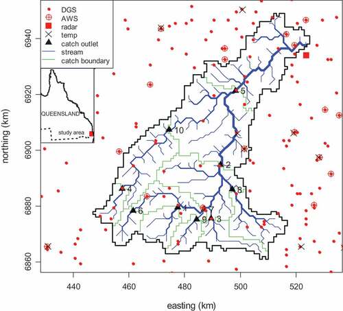
The climate of the region is subtropical, with an average temperature of 26.5°C, and annual mean rainfall of about 990 mm with an average of 124 wet days per year. In general, the summer months from December to February are hot and humid, while winter months from June to August are moderately dry. According to the Köppen-Geiger climate classification (Peel et al. 2007), the region falls under Cfa (temperate, without dry season and hot summer). Maximum daily temperature has significant effects on the sub-daily rainfall characteristics (Gyasi-Agyei 2013). Within the study area there are 15 temperature stations, but only two are located within the Logan catchment. For each day, the IDW method was used to interpolate the maximum daily temperature values over the 1 km × 1 km radar grids, and those within the catchment averaged as the representative value.

Topographic information required by the distributed rainfall–runoff model were obtained from a digital elevation model (DEM). The 30 m × 30 m pixel size DEM available was averaged over 1 km × 1 km grid resolution to conform to the rainfall radar grid, and also to speed up simulation runs. The approach of the single flow direction of steepest descent to one of the eight neighbours, after filling depressions to create the best artificial paths, implemented in GRASS software (called from R function rgrass7; Bivand 2017), was adopted to develop the flow directions. The flow direction raster was then used to derive a raster consisting of accumulated areas of each pixel. An arbitrary support area (minimum area for channel initiation) of 5 km² was used to delineate the drainage network (Fig. 1). There are 10 discharge measuring stations (Table 1), consisting of six headwater catchments (93–232 km²) and four larger nested catchments (446–2513 km²), but their available discharge data² vary in time and have missing data.

Table 1. Basic features of the catchments and the mean and maximum pixel distance (km) from daily gauge stations (DGS) and automatic weather stations (AWS). MDO: maximum distance to catchment outlet; EC: elongation coefficient; NE: number of rainfall–runoff events

Catchment no.	MDO (km)	Area (km^2)	EC	No. of DGS	No. of AWS	DGS (km)		AWS (km)		NE
						mean	max	mean	max
1	22.31	154	0.63	0	0	6.6	12	11.2	15	0
2	67.36	1360	0.62	18	2	4.6	12	11.2	21.2	0
3	30.14	153	0.46	1	0	6.2	9.2	12.7	18.4	0
4	16.9	93	0.64	4	0	2.1	4.1	13	19.9	11
5	101.57	2513	0.56	31	3	4.5	12	11.7	22.4	15
6	15.49	98	0.72	0	0	6.5	10.8	13.2	20.2	9
7	47.46	553	0.56	7	1	4.8	12	9.4	20.2	11
8	28.21	232	0.61	5	0	3.5	7.1	16.1	21.2	14
9	17.56	109	0.67	2	0	4	7.3	10.1	14	3
10	52.94	446	0.45	7	0	3.7	9.4	11	21.4	4
11	137.44	3088	0.46	40	5	4.3	12	11.2	22.4	-

The elongation coefficient, defined as the ratio of the diameter of a circle of equivalent area to the maximum catchment length, for the catchments varies. Schumm (1956, p. 612) used the elongation coefficient to classify catchments as “circular” (0.9–1), “oval” (0.8–0.9), “less elongated” (0.7–0.8), “elongated” (0.5–0.7), and “more elongated” (<0.5). This parameter is important as highly elongated catchments tend to result in increased travel time, thus attenuating the hydrograph. For each pixel, the overland flow distance to the channel network and also to the catchment outlet was computed for use by the distributed rainfall–runoff model. Table 1 presents some basic features of the catchments. All the catchments are “elongated”, with one being “more elongated”. Table 1 also shows the number of DGS and AWS stations within the catchments, and the mean and maximum distances of the catchment pixels from the gauging stations.

Not all catchments have flow records without missing data for each storm event. Therefore, for each storm event only catchments without missing flow data were considered, labelling an event on a catchment as a catchment event. However, catchment events are referred to as events for simplicity. Storm events are separated by a minimum of 24 dry hours, but could span several wet days. Baseflow was separated from the total hydrograph using the constant-baseflow method (Chin 2013, p. 483), and the surface runoff hydrograph was modelled in this paper. The distribution of the 67 events selected is shown in Table 1, noting that there were no good data for catchments 1–3. To show the characteristics of the selected events, rainfall amounts for each hour were averaged over the pixels to obtain a catchment average time series. Dry proportion was then estimated as the fraction of time that there was no rainfall. Table 2 shows that the essential characteristics span a broad spectrum of rainfall and runoff, demonstrating that the events varied considerably. Altogether 72 unique daily rainfields generated the 67 selected storm events.

Table 2. Rainfall and runoff statistics for the 67 selected catchment events

Statistics	Rainfall					Runoff
	Depth (mm)	Duration (h)	Intensity (mm h^−1)		Proportion dry (-)	Depth (mm)	Duration (h)	Peak (m^3 s^−1)	Time to peak (h)
			Ave.	Max.
Minimum	1.3	7.0	0.05	0.45	0.000	1.0	32.0	2.5	9.0
First quarter	22.6	24.0	0.71	4.56	0.014	4.1	63.0	15.0	35.0
Median	38.8	37.0	1.28	6.93	0.130	8.4	87.0	40.9	46.0
Mean	55.5	42.4	1.40	8.39	0.196	19.1	90.6	110.3	52.4
Third quarter	87.4	58.5	1.75	11.97	0.298	14.8	109.0	124.3	65.5
Maximum	178.1	156.0	3.73	21.72	0.735	109.6	215.0	1071.3	171.0

3 Methodology

3.1 Daily rainfields

The model presented by Gyasi-Agyei (2018), which was built on the earlier work of Gyasi-Agyei and Pegram (2014) and Gyasi-Agyei (2016), was adopted to generate the daily rainfields from point daily rainfall records. It is an ordinary kriging-based interpolation on quantile-quantile (Q-Q) transformation of the daily rainfall data into normal scores which follows the standard Gaussian distribution. The details of the parameter estimation of the daily rainfield model are given in Gyasi-Agyei (2018). However, the major processes involved in its application are given below.

The raingauge collocated daily rainfall amounts greater than zero for the day of interest are transformed into probabilities using one of seven common two-parameter distributions (log-logistic, kappa, generalized Pareto, Gumbel, log-normal, Weibull and gamma) that can capture rightly skewed data such as daily rainfall amounts (e.g. Buishand 1978, Groisman et al. 1999, Shoji and Kitaura 2006). Other researchers have suggested a higher number of parameter distributions to be more appropriate. For example, Wilks (1998) suggested using the three-parameter mixed exponential distribution, and Hanson and Vogel (2008) the four-parameter kappa distribution. The best distribution for wet days is selected based on the p value of the Anderson-Darling statistic. The selected distribution is zero inflated to account for zeros in the daily records before transforming the probabilities into the normal scores w[s_k] as:

(1) $w\left[s_k\right]=\begin{array}{c}{\mathrm{\Phi }}^{-1}\left[F_R\left(r\left[s_k\right]\right)(1-p_0)+p_0\right],r\left[s_k\right]>0\\ {\mathrm{\Phi }}^{-1}\left[p_0.exp\left(-\frac{d[s_k]}{\bar{d}}\right)\right],r\left[s_k\right]=0\end{array}$(1)

where F_R(r[s_k]) is the probability generated from the selected distribution (F_R) from the rainfall amount r[s_k] at station k with coordinates s_k ; p₀ is the probability of no rain, defined as the number of raingauges of zero reading over the total number of raingauges; d[s_k] is the distance of a zero reading raingauge from the nearest wet raingauge; $\bar{d}$ is the average of d; and $\mathrm{\Phi }$ is the cumulative normal distribution N(0,1). Inversion of Equation (1)(1) $w\left[s_k\right]=\begin{array}{c}{\mathrm{\Phi }}^{-1}\left[F_R\left(r\left[s_k\right]\right)(1-p_0)+p_0\right],r\left[s_k\right]>0\\ {\mathrm{\Phi }}^{-1}\left[p_0.exp\left(-\frac{d[s_k]}{\bar{d}}\right)\right],r\left[s_k\right]=0\end{array}$(1) leads to the rainfall amount for a simulated normal score as:

(2) $r\left[s_k\right]=\begin{array}{c}{F_R}^{-1}\left[\left\{\mathrm{\Phi }\left(w\left[s_k\right]\right)-p_0\right\}/(1-p_0)\right],\mathrm{\Phi }\left(w\left[s_k\right]\right)\ge p_0\\ 0,\mathrm{\Phi }\left(w\left[s_k\right]\right)<p_0\end{array}$(2)

The sample correlogram $\tilde{R}\left(i,j\right)$ of the raingauge collocated data is estimated as:

(3) $\tilde{R}\left(i,j\right)=\frac{1}{N_h}\sum _{k=1}^{N_h}w[s_k]w[s_k+h]-m_0{m}_{+h},\mathrm{\forall }(s_k,s_k+h):h\in \left[i\pm 1,j\pm 1\right]$(3)

where N_h is the number of contributing raingauge pairs separated by distance h that falls within the bounded region of [i ± 1, j ± 1]; m₀ and m_+h are the means of the pair of tail w[s_k] and head w[s_k+h] values. The Yao and Journel (1998) “round-trip” fast Fourier transform approach with intermediate smoothing processes is applied to the sample correlogram. Analysis of radar rainfall data in South Africa (Gyasi-Agyei and Pegram 2014) and in Australia (Gyasi-Agyei 2016) indicated that a three-parameter (L_u, L_v, θ) two-dimensional (2D) exponential distribution expressed as:

(4) $\begin{array}{rl}& R_{\mathrm{\Theta }}(x,y)=R_{\mathrm{\Theta }}(u,v)\\ & =exp\left\{-{\left[{\left(\frac{u}{L_u}\right)}^2+{\left(\frac{v}{L_v}\right)}^2\right]}^{\frac{1}{2}}\right\},\\ & u=y\left(\theta \right)+x\mathrm{c}\mathrm{o}\mathrm{s}\left(\theta \right)\\ & v=y\mathrm{c}\mathrm{o}\mathrm{s}\left(\theta \right)-x\mathrm{s}\mathrm{i}\mathrm{n}\left(\theta \right)\end{array}$(4)

fitted the correlogram very well. In Equation (4)(4) $\begin{array}{rl}& R_{\mathrm{\Theta }}(x,y)=R_{\mathrm{\Theta }}(u,v)\\ & =exp\left\{-{\left[{\left(\frac{u}{L_u}\right)}^2+{\left(\frac{v}{L_v}\right)}^2\right]}^{\frac{1}{2}}\right\},\\ & u=y\left(\theta \right)+x\mathrm{c}\mathrm{o}\mathrm{s}\left(\theta \right)\\ & v=y\mathrm{c}\mathrm{o}\mathrm{s}\left(\theta \right)-x\mathrm{s}\mathrm{i}\mathrm{n}\left(\theta \right)\end{array}$(4) , x and y are the horizontal and vertical separation distances from the centre; u and v are the separation distances along the major and minor axes, respectively, of the elliptical contour; θ is the angle between the major axis and the horizontal direction; anisotropy is the ratio of the major axis length (L_u) to the minor axis length (L_v). Note that, in real applications, only the raingauge collocated data are available. However, Gyasi-Agyei (2016) established linkages between the observed (referred to as complete) radar parameters that are required and the raingauge collocated parameters of Equation (4)(4) $\begin{array}{rl}& R_{\mathrm{\Theta }}(x,y)=R_{\mathrm{\Theta }}(u,v)\\ & =exp\left\{-{\left[{\left(\frac{u}{L_u}\right)}^2+{\left(\frac{v}{L_v}\right)}^2\right]}^{\frac{1}{2}}\right\},\\ & u=y\left(\theta \right)+x\mathrm{c}\mathrm{o}\mathrm{s}\left(\theta \right)\\ & v=y\mathrm{c}\mathrm{o}\mathrm{s}\left(\theta \right)-x\mathrm{s}\mathrm{i}\mathrm{n}\left(\theta \right)\end{array}$(4) .

For the complete radar, the Gumbel copula was used to model the joint distribution of L_u and L_v, its parameter varying with the maximum temperature of the day with a stronger dependence at lower temperatures. The copula margins follow the Box-Cox power exponential distribution (Rigby and Stasinopoulos 2004). However, the values of L_u and L_v of the raingauge collocated data and the maximum temperature of the day were used as covariates for predicting the margin distribution parameters within the framework of GAMLSS (generalized additive models for location, scale and shape), using the R package gamlss (Stasinopoulos and Rigby 2007). The correlogram direction, being independent, is modelled with a second-order harmonic distribution.

With the complete radar correlogram parameters, ordinary kriging (Cressie 1993) was performed to produce the Gaussian mean and standard deviation for each grid cell. Then the joint sequential simulation of multi-Gaussian fields methodology proposed by Gómez-Hernández and Journel (1993) was used to simulate random fields of the normal score conditioned on the raingauge (collocated) data before converting into rainfall through the Q-Q transformation of Equation (2)(2) $r\left[s_k\right]=\begin{array}{c}{F_R}^{-1}\left[\left\{\mathrm{\Phi }\left(w\left[s_k\right]\right)-p_0\right\}/(1-p_0)\right],\mathrm{\Phi }\left(w\left[s_k\right]\right)\ge p_0\\ 0,\mathrm{\Phi }\left(w\left[s_k\right]\right)<p_0\end{array}$(2) . This task was performed using the R package gstat (Pebesma 2004).

At this stage we are able to generate daily rainfields from point daily rainfall data. The next section discusses how to generate pixel-wise hourly proportions (fragments) for disaggregating the gridded daily rainfall amounts into hourly rainfields conditioned on the observed daily and limited hourly data.

3.2 Generation of hourly rainfields

There are in total 32 AWS stations within the 150 km × 150 km region, with only five located within the Logan catchment. Only those AWS stations that recorded rain were used in the analysis, noting that radar collocated hourly data were used in lieu. Including AWS stations with all zero readings may yield all zero hourly proportions for sites where the daily raingauges may suggest otherwise. Note in passing that zero daily rain would assign zero rain for all the hourly time intervals anyway. All the AWS data were scaled by their daily totals to obtain proportions of rain that occurred during the hourly intervals to obtain scaled storm profiles. In essence, the hourly proportional approach is a variant of the MOF. Gyasi-Agyei (2012) used observed scaled storm profiles for disaggregating point daily rainfall time series to sub-hourly time scale in different climatic zones. He prepared a pool of observed scaled storm profiles and used some rules to select the appropriate one for the given day.

Six options for deriving the hourly proportions were considered in this study:

1. for each pixel, use the actual radar proportions – the ORI option;

2. for each pixel, select the nearest AWS station, and this is equivalent to IDW using only one neighbour – the IDW1 option;

3. for each hour, the observed proportions are interpolated independently over the 1 km × 1 km grid of the whole region using the IDW method and a maximum of three neighbours – the IDW3 option;

4. for each pixel, select the AWS station that has the minimum absolute difference of the pixel and the AWS daily amounts – the DEP option;

5. for each pixel, rank the AWS by distance (1 for closest) and absolute difference of amounts as in option 4, average the two ranks and select the AWS with the minimum average rank – the COM option; and

6. for each pixel, the scaled storm profile is randomly selected from the available AWS stations – the RAN option.

Multiplication of the pixel-wise hourly proportions to the generated pixel-wise daily total gives the hourly rainfields. This is a case of spatio-temporal daily rainfall disaggregation into hourly rainfields conditioned on DGS and AWS. Options 4–6 performed poorly during the initial analysis, so they were discarded. It is not surprising that options 4–6 were not ideal because, unlike options 1–3 they lack the spatial pattern of rainfall. Combination of the first three options for determining the disaggregation proportions with the original pixel daily amounts and simulated daily amounts leads to six versions of hourly rainfields to serve as input to the rainfall–runoff model:

1. ORI-ORI: actual daily amount + ORI option;

2. SIM-ORI: simulated daily amount + ORI option;

3. ORI-IDW1: actual daily amount + IDW1 option;

4. SIM-IDW1: simulated daily amount + IDW1 option;

5. ORI_IDW3: actual daily amount + IDW3 option;

6. SIM-IDW3: simulated daily amount + IDW3 option.

These six rainfields are different versions of rainfall input into the rainfall–runoff model, noting that ORI-ORI is referred to as the complete or the observed rainfall.

3.3 Spatial rainfall organization statistics

The spatial organization of the rainfields was examined using two groups of statistics. The first group of statistics are as presented by Zanon et al. (2010), which were developed upon the work of Woods and Sivapalan (1999), Viglione et al. (2010) and Zoccatelli et al. (2010). They are based on the mean and variance of rainfall weighted by the flow distance to the catchment outlet. Both of these indices use the weight function, w(x,y,t), defined as:

(5) $w(x,y,t)=\frac{P(x,y,t)}{A^{-1}{\int }_{A}P(x,y,t)\mathrm{d}A}$(5)

where P(x,y,t) is the rainfall at location x, y and time t, and A is the catchment area. The first spatial pattern parameter is the normalized time distance at time t, θ₁(t), defined as:

(6) ${\theta }_1(t)=\frac{{\int }_{A}w(x,y,t)\tau (x,y)\mathrm{d}A}{A{\tau }_m}$(6)

and the second is the normalized time dispersion parameter, θ₂(t), defined as:

(7) ${\theta }_2(t)=\frac{{\left\{{\int }_{A}w(x,y,t){\left[\tau (x,y)-{\theta }_1(t){\tau }_m\right]}^2\mathrm{d}A\right\}}^{0.5}}{{\left\{{\int }_A{\left[\tau (x,y)-{\tau }_m\right]}^2\mathrm{d}A\right\}}^{0.5}}$(7)

where θ_m is the mean travel time, and θ(x,y) is the travel time to the catchment outlet.

When the rainfall distribution is either homogeneous or concentrated close to the mean, θ₁(t) takes on values close to 1. A value of θ₁(t) < 1 signifies that rainfall is distributed near the catchment outlet, leading to the hydrograph passing the outlet quicker than in the case of spatially uniform rainfall. The opposite case, where θ₁(t) > 1, implies rainfall is concentrated towards the headwater portion of the catchment, and the hydrograph is delayed compared with the spatially uniform rainfall case. With regards to θ₂(t), a value of 1 indicates spatially uniform rainfall and θ₂(t) < 1 suggests a concentration of, or unimodal, rainfall anywhere in the catchment. A value of θ₂(t) > 1 may suggest multimodal peaks, and the rainfall may be concentrated at both the headwaters and the catchment outlet. On the same day, rainfall could be highly variable across the catchment and that could significantly affect the generation of runoff.

Emmanuel et al. (2015) presented the second group of spatial statistics, which are essentially comparing the catchment width function and the rainfall width function. The catchment width function is defined as the proportion of the catchment area at a given distance from the outlet (equivalent to spatially uniform rainfall), whereas the rainfall width function is the proportion of rainfall falling on the catchment at a given distance from the outlet. A cumulative distribution plot of these functions is used to estimate the required statistics. Statistic VG is defined as the absolute maximum distance between the cumulative plots and HG is the corresponding horizontal difference scaled by the maximum distance to the outlet of the catchments; VG takes on values close to zero when the rainfall displays insignificant spatial distribution, whereas a higher value is an indication that the rainfall is distributed on a small part of the catchment. For cases where the rainfall is uniformly distributed or concentrated near the catchment centre, HG takes on values close to zero. A negative value of HG is for the case where rainfall is distributed downstream and a positive value indicates it is distributed upstream. We used VHG, the diagonal deviation, which is the square root of the sum of squares of VG and HG.

3.4 The rainfall–runoff model

A simplified GIS-based distributed rainfall–runoff model was adopted. The rainfall is partitioned into infiltration, f(t) (mm h⁻¹), and rainfall excess, u(t) (mm h⁻¹), at the pixel scale (1 km × 1 km spatial resolution) using two models; the first one is the Philip two-parameter model (Philip 1957), expressed as:

(8) $f(t)=\frac{1}{2}S{t}^{-1/2}+C$(8)

where S (mm h^−1/2) is the sorptivity, which is a function of the soil suction potential; and C (mm h⁻¹) is the constant infiltration. For the second infiltration model, an initial loss (IL) (mm) is accounted for before the beginning of the surface runoff, and constant continuing loss (CL) (mm h⁻¹) occurs from the onset of surface runoff to the end of the rainfall event. This model is expressed mathematically as:

(9) $f(t)=\begin{array}{c}u(t)\mathrm{f}\mathrm{o}\mathrm{r}\underset{0}{\overset{t}{\int }}u(t)\mathrm{d}t\le \mathrm{I}\mathrm{L}\\ \begin{array}{c}\left[\mathrm{I}\mathrm{L}-\underset{0}{\overset{t-dt}{\int }}u(t)\mathrm{d}t\right]/\mathrm{d}t\mathrm{f}\mathrm{o}\mathrm{r}\underset{0}{\overset{t-dt}{\int }}u(t)\mathrm{d}t<\mathrm{I}\mathrm{L}\mathrm{a}\mathrm{n}\mathrm{d}\underset{0}{\overset{t}{\int }}u(t)\mathrm{d}t>\mathrm{I}\mathrm{L}\\ max\left[u(t)-\mathrm{C}\mathrm{L},0\right]\mathrm{f}\mathrm{o}\mathrm{r}\underset{0}{\overset{t-dt}{\int }}u(t)\mathrm{d}t>\mathrm{I}\mathrm{L}\mathrm{a}\mathrm{n}\mathrm{d}\underset{0}{\overset{t}{\int }}u(t)\mathrm{d}t>\mathrm{I}\mathrm{L}\end{array}\end{array}$(9)

Although the catchment is heterogeneous in terms of surface cover, soils and infiltration properties in general, the assumption of homogeneous infiltration model parameters does not defeat the purpose of examining the runoff response from different versions of rainfall input, be it the observed radar or hourly rainfields simulated from collocated radar data.

The surface runoff produced at the pixel level is routed to the catchment outlet, following the pixel-wise direction of steepest descent, using the Hayami kernel function, K(t). It is an analytical solution of the diffusive wave equation and a special case where both the convective (celerity) parameter V (km h⁻¹) and the diffusivity parameter D (km² h⁻¹) are considered constant over the catchment during the rainfall event. The mathematical expression is given as (Moussa 1996):

(10) $K_i(t)=\frac{L_i}{2{\left(\pi D\right)}^{1/2}{t}^{3/2}}exp\left[\frac{V{L}_i}{4D}\left(2-\frac{L_i}{Vt}-\frac{Vt}{L_i}\right)\right]$(10)

where L_i (km) is the distance of pixel i from the catchment outlet, and t is time in hours. For given net rainfall intensities of the pixels, u_i(t) (mm h⁻¹), the catchment outflow discharge, Q(t) (m³ s⁻¹), is given by the convolution integral as:

(11) $Q(t)=\frac{{10}^{-3}\mathrm{\Delta }A}{3600}\sum _{i=1}^N{\int }_0^t{u}_i(t)K_i(t-\tau )\mathrm{d}\tau$(11)

where ΔA is the area (m²) of a pixel and N is the number of pixels of the catchment. It was observed that the simulated hydrographs were lagging behind the observed, so a lag time, Lag (h), to shift the hydrograph some hours was introduced. The lag time could vary depending on the spatial and temporal distribution of the rainfall event, and the catchment initial moisture spatial distribution. This leads to the rainfall–runoff model having five parameters, which were calibrated for each event separately by minimizing the sum of square deviations between the observed and the simulated hydrograph from the complete radar data. The shuffled complex evolution (SCE) method of Duan et al. (1992), implemented in R function sceua (Skøien et al. 2014) was used for the parameter identification. With the calibrated parameters, the other rainfall data versions were run through the rainfall–runoff model to obtain their respective hydrographs. All six simulated hydrographs of the rainfall input versions for each event were then evaluated against the observed hydrograph. A simulation time step of 5 min was used. Therefore, the rainfall intensities were repeated within the hour at an interval of 5 min and the flow data were interpolated at the same time step.

4 Results and discussion

4.1 Rainfields

The numbers of the 72 daily rainfields following the various two-parameter distributions are: five for log-logistic, seven for kappa, eight for generalized Pareto, one for Gumbel, four for log-normal, 24 for Weibull, and 23 for gamma. This demonstrates that the marginal distribution of the wet amounts of daily rainfall varies considerably. Also, the number of operational daily raingauges within the square region for the 72 wet days varied between 190 and 243.

We first compare some statistics of the marginal distribution of the observed (complete radar) and raingauge collocated simulated rainfields, and the spatial correlation within the square region. Figure 2 shows that the dry proportion (the ratio of pixels with rainfall amount <1 mm to the total number of pixels) was preserved very well. This is also true for the mean amounts, as the values lie very close to the line of perfect agreement. However, the rainfall variance values seem to be underestimated for some wet days. This is largely due to the fewer than 250 raingauge stations used, a raingauge density of 1 per 90 km², which is not adequate to capture the higher moments properly. The daily raingauge network density should be better than one raingauge per 16 km² to capture the spatial variability properly (Gyasi-Agyei and Pegram 2014). It needs to be stressed that the raingauge collocated rainfall amount distribution is not necessarily the same as that of the complete radar due to the low network density.

Figure 2. Comparison of the observed (OBS) and the average simulated (SIM) dry (amounts < 1mm) proportions, mean and variance of the 72 daily rainfields of the square region. The solid line is for perfect agreement

Figure 3 presents a comparison of the correlograms of three wet days. The correlogram values $C\left(\overline{h_j}\right)$ were estimated as:

(12) $C\left(\overline{h_j}\right)=\frac{1}{{\sigma }^2{N}_j}\sum _{i=1}^{N_j}\left(r[s_i].r[s_i+h]\right)-m_{{ }_j}^2,\mathrm{\forall }(s_j,s_j+h):h\in (h_j,h_j+2)$(12)

Figure 3. Comparison of the observed (OBS) and simulated (SIM) correlogram of the square rainfield. SIM indicates the 20 individual simulations and SIM-AVE represents the average values at the lag distances

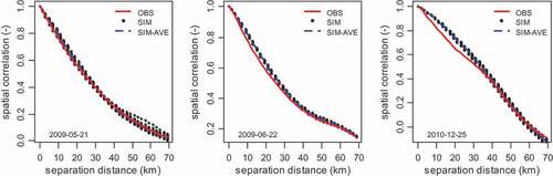
where r[s_i] is the rainfall amount at location s_i; σ² is the rainfield variance; N_j is the number of paired sites within the separation distance h; and m_j and $\overline{h_j}$ are the average of r and h of all N_j paired sites, respectively. It is observed that the correlograms were preserved quite well and there were no significant variations of the 20 simulation runs. Also of note are the different correlograms for different wet days. However, it is noted that only the expected spatial structure was analysed, and no information on the higher-order statistics (e.g. variance, skewness) is provided.

Adjustment of the raingauge collocated rainfall amount distribution is required in future studies to better reflect the spatial structure of the complete radar rainfield. Koutsoyiannis et al. (2011) argued that a power-law-type 2D spatial structure may be more appropriate for rainfall, and future work will look into this. It is yet to be seen how the errors in the simulated daily rainfields are propagated to the runoff errors of the events.

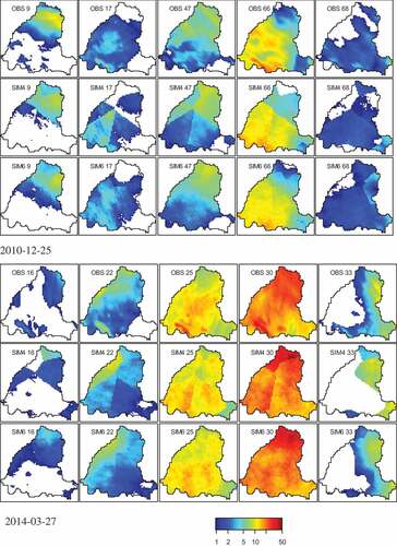
Table 2 shows some rainfall and runoff statistics of the 67 selected events. Two storm events of 25–27 December 2010 (from 9am 2010-12-24 to 9am  2010-12-27) and 27–28 March 2014 (from 9am 2014-03-26 to 9am  2014-03-28) have been selected for discussion of the results before looking into the aggregated results of all the 67 events. These events have data for, respectively, six and five catchments of different size and shape. Hereafter they are referred to as the event of 2010-12-25 and 2014-03-27, respectively. Figure 4 compares the event total rainfall amounts of the complete radar and the first three simulated rainfields. The observed radar image exhibits a narrow band of supercells at the southwest corner, particularly over catchments 1 and 6, where there are no raingauges so rainfall amounts could not be detected. It is not certain whether it is an artefact of the radar data processing. Interpolation methods have great difficulty mimicking such occurrences where there are no raingauges, highlighting the need for an increase in raingauge network density. Selected hourly rainfields of the two events of the complete radar and those of SIM-IDW1 and SIM-IDW3 are presented in Figure 5. While both options simulated the rainfields very well, SIM-IDW1 shows artefacts of sharp transition lines. It is clear that the beginning and the end of the storms are well captured. This is also true for the dry patches.

Figure 4. Comparison of the event total rainfall amounts (mm) of the complete radar (OBS) and the first three simulated (SIM) rainfields. Top row: the event of 2010-12-25 and bottom row: the event of 2014-03-27

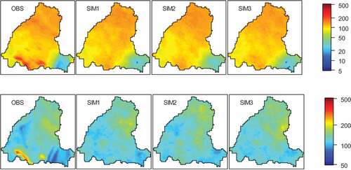
Figure 5. Comparison of hourly rainfields (mm) of the complete hourly radar (OBS) and of the first simulated rainfields using SIM-IDW1 (middle row) and SIM-IDW3 (bottom row). The numbers indicate the hours since 09:00 h on 24 December 2010 and 26 March 2014

The spatial statistics of the total rainfall amounts of the 67 events are shown in Figure 6. There is a resemblance between the spatial organization of the simulated and the observed rainfields as the correlations of the normalized time distance and the normalized time dispersion parameters are in excess of 0.91. Also, the points are well distributed on both sides of the line of perfect agreement, though there is evidence of underestimation of some events. For the statistics comparing the width function VHG (Fig. 6, top right), the correlation is 0.85 and the points are scattered around the line of perfect agreement. Clearly, the events exhibit significantly different spatial structure as θ₁ less than 1 suggests rainfall is distributed near the catchment outlet, around 1 suggests fairly uniformly distributed and above 1 suggests it is concentrated towards the headwater portion. Values of θ₂ spread on either side of 1 suggest some events are concentrated anywhere within the catchment, and some are multimodal (Zanon et al. 2010). These observations are also supported by the values of VG and HG presented as VHG in Figure 6.

Figure 6. Comparison of the event total rainfall amount spatial statistics for the complete radar (OBS) and the simulated (SIM) rainfields of the 67 events. The lines of perfect agreement are shown as dashed (red) lines

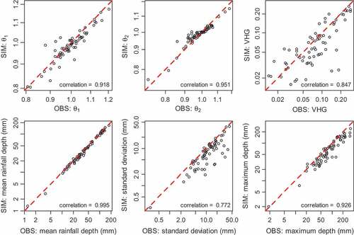
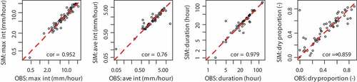
The events’ average rainfall amounts are very well reproduced, but there is a problem with the maximum rainfall amounts. With interpolation methods, it is difficult to model the maximums if they are not captured by the installed raingauges. Occurrence of supercells, such as shown in Figures 4 and 5, and dry patches that do not pass over the raingauges will lead to underestimation of the maximum, and perhaps overestimation of the minimum. This will lead to underestimation of the standard deviation as shown in Figure 6 (second row, second column). Also, rainfall intensities for each hour were averaged over the pixels to obtain a catchment average time series for each event, considering intensities less than 0.1 mm h⁻¹ as dry. Figure 7 compares the statistics of the generated time series of the observed and the simulated rainfall. The time series statistics are satisfactorily reproduced.

Figure 7. Comparison of the statistics for the 67 events of the observed and the simulated rainfall. The lines of perfect agreement are shown as dashed (red) lines

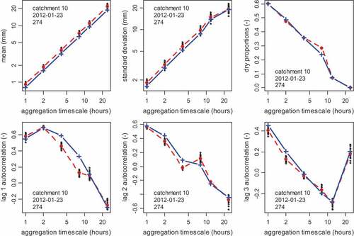
The event of 2012-01-23 on catchment 10 was caused by seven continuous wet days, the longest wet spell, so it was used to assess the reproduction of continuous rainfall time series statistics at aggregation levels of 1, 2, 4, 8, 12 and 24 h. Due to space consideration, the statistics of only pixel number 274 are shown in Figure 8. There is not much difference between the values of the 20 simulation runs. For this pixel, all statistics were preserved reasonably well, although there is a slight overestimation of the mean and variance, and underestimation of the autocorrelations. The sudden increase in the lag-3 autocorrelation at 24-h aggregation level could be an artefact due to the limited number of sampling points at this time scale. The next section assesses how the uncertainties in the simulated rainfields affect the simulated hydrographs.

Figure 8. Statistics of different levels of aggregation time scale of pixel 274 for catchment 10 event of 2012-01-23, which has the longest rainfall duration of seven continuous wet days. Solid (blue) lines with crosses are the complete radar; black dots are the 20 simulation runs, and the dashed (red) lines are the average of the 20 simulation runs

4.2 Runoff

Table 3 presents the average values of the rainfall–runoff model calibrated parameters of each catchment using the complete radar rainfall. For each event, the average of 20 simulated hydrographs derived from the six rainfall versions using the calibrated parameters was compared against the observed hydrograph. Performance statistics of absolute percentage error in runoff depth (ERD), peak discharge (EPD) and time to peak (ETP), and the Nash-Sutcliffe efficiency (NSE), were used to assess the simulated hydrographs. These performance statistics are defined as:

(13) $\mathrm{E}\mathrm{R}\mathrm{D}=100\left(\frac{\left|D^o-D^s\right|}{D^o}\right)$(13)

(14) $\mathrm{E}\mathrm{P}\mathrm{D}=100\left(\frac{\left|Q_p^o-Q_p^s\right|}{Q_p^o}\right)$(14)

(15) $\mathrm{E}\mathrm{T}\mathrm{P}=100\left(\frac{\left|T_p^o-T_p^s\right|}{T_p^o}\right)$(15)

(16) $\mathrm{N}\mathrm{S}\mathrm{E}=1-\frac{\sum _{i=1}^n{(Q_i^o-Q_i^s)}^2}{\sum _{i=1}^n{(Q_i^o-Q_m^0)}^2}$(16)

Table 3. Catchment average and standard deviation (SD) of the calibrated parameters. IL: initial loss; CL: continuing loss; V: celerity; D: diffusivity

Catchment no.	IL (mm)		CL (mm h^−1)		V (km h^−1)		D (km^2 h^−1)		Lag (h)
	Mean	SD	Mean	SD	Mean	SD	Mean	SD	Mean	SD
4	21.3	13.1	2.33	2.87	1.42	1.20	9.8	7.1	13.3	3.6
5	28.9	26.3	5.42	4.75	1.89	0.90	15.0	9.5	15.8	5.9
6	12.8	8.1	1.40	1.19	0.64	0.47	6.6	7.8	11.5	5.9
7	22.4	18.5	3.82	4.58	1.52	0.78	8.6	5.7	12.0	7.1
8	19.2	24.6	3.16	3.71	1.65	1.23	12.3	10.3	15.6	3.6
9	31.3	22.0	6.12	6.58	1.20	0.30	9.1	4.6	13.1	0.9
10	47.4	54.0	3.06	3.71	1.35	0.91	10.7	9.8	18.8	5.5

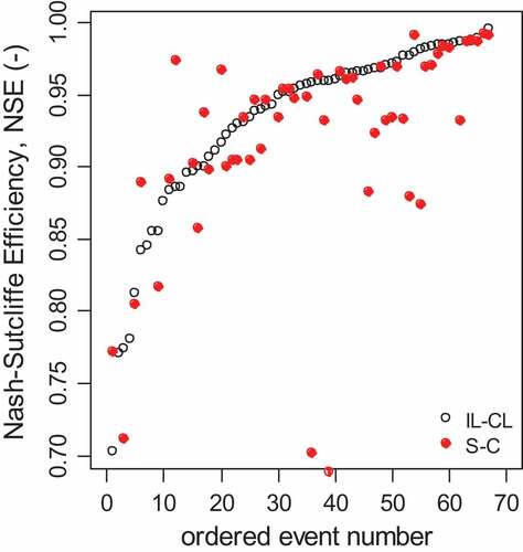
where D, Q_p, T_p, Q_m and Q_i are the runoff depth, peak, time to peak, mean discharge and discharge at time step i, respectively. Superscript o refers to the observed and s the simulated rainfield hydrographs. The NSE takes on values from −∞ to 1, 1 being a perfect match, and less than 0 indicates that the observed mean is a better predictor than the model. The NSE values shown in Figure 9 indicate that the infiltration model IL-CL outperformed S-C in 69% of the 67 events analysed. Hence, only the IL-CL infiltration model is considered in the ensuing.

Figure 9. Comparison of the Nash-Sutcliffe efficiency (NSE) performance statistics of the two infiltration models: initial loss – continuing loss (IL-CL), and Philip sorptivity – constant infiltration (S-C). Event numbers are ordered in increasing NSE value for the IL-CL model to improve readability

The uncertainties in rainfall propagated in runoff errors were analysed at three different levels:

• AMOUNT: due to the daily totals simulation only being obtained by using the simulated daily totals and the complete radar hourly proportions at each pixel, compare hydrographs of ORI-ORI and SIM-ORI;

• PROP: due to the hourly proportions only being obtained by using the complete radar daily totals at each pixel combined with the two options for generating the hourly proportions, compare hydrographs of ORI-ORI, ORI-IDW1 and ORI-IDW3; and

• AMOUNT+PROP: due to a combination of the AMOUNT and PROP sources of uncertainties, compare hydrographs of ORI-ORI, SIM-IDW1 and SIM-IDW3.

4.2.1 Individual events

Figure 10 exhibits the simulated hydrographs of the selected events that had the highest number of catchments with flow data. Due to the inability to capture the supercell during the event of 2014-03-25 within the headwater catchments 1 and 6, catchment 7 (encompassing these catchments) recorded the worst performance in reproducing the observed hydrographs. Using SIM-IDW1, catchment 7 registered ERD of 43.9%, EPD of 26.5%, ETP of 2.9% and NSE of 0.83. Values for catchment 10 were 12.5%, 61.8%, 4.3% and 0.83, respectively, while the averages of the four remaining catchments were 9.3%, 11.3%, 4.3% and 0.92, respectively. These values are not significantly different from those of SIM-IDW3.

Figure 10. Comparison of the observed and simulated hydrographs of the different catchments using the calibrated parameters and the different rainfall sources. Time in hours since 09:00 h on 24 December 2010 and 26 March 2014

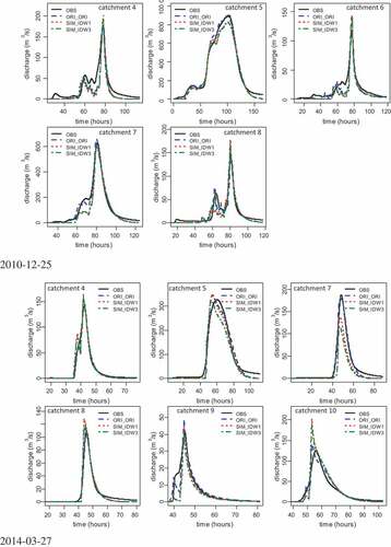
The exercise in this paper is to ascertain how much the performance statistics are degraded by using the different simulated rainfall versions. Hence the performance statistics are reported relative to those of the complete radar. For the 2014-03-25 event, the average values of all the catchments using the complete radar were ERD of 4.7%, EPD of 10.8%, ETP of 3.4% and NSE of 0.97. Compared with these results, using SIM-IDW1 resulted in increases in values of ERD (10.9%), EPD (11.4%) and ETP (0.6%), while NSE reduced to 0.89. With regard to the event of 2010-12-25, catchment average changes in the performance statistics were ERD of 6.7%, EPD of 6.3%, and ETP of −0.3%, with the NSE reduced by 0.03 from 0.93, which showed better performance than for the previous event. Assessing the effects of rainfall variability on runoff using individual events could lead to misinterpretation of results (Mandapaka et al. 2009), so combined events were examined, as described in the next section.

4.2.2 Combined events

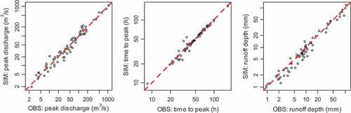
The statistics of the observed hydrographs were compared with those simulated using the SIM-IDW1 rainfall version, as shown in Figure 11 for all 67 events. Underestimation of the runoff depth is demonstrated for some events, particularly those with depths less than 20 mm. This is primarily due to the fact that smaller rainfall events are more sensitive to the infiltration parameters, which are subject to the initial moisture conditions. However, the peaks and times to peak seem to be very well predicted, and are scattered nearly evenly on both sides of the line of perfect agreement.

Figure 11. Comparison of variables of the observed and simulated hydrographs using rainfall source SIM-IDW1 for all 67 catchment events. The lines of perfect agreement are shown as dashed (red) lines

In order to remove the influence of the spatial pattern of just one event, the events were grouped into four classes of the observed runoff depth (ORD). Rainfall and runoff characteristics given in Table 4 were checked, but only the ORD could give a reasonable classification. Table 5 presents the groups’ average performance statistics of the simulated hydrographs using the complete radar rainfall version (ORI-ORI). In general, the fit of the rainfall–runoff model using the complete radar data was good, with an average value of NSE over 0.93. The average ERD was under 8%, the highest ORD group yielding the lowest ERD value of 5.8%. For the EPD, the two lowest ORD groups recorded 13.1%, while the highest ORD group registered below 10%, with the overall average being 11.8. A similar trend was observed for the ETP, where the highest ORD recorded 1.5% and the lowest ORD gave 5%, with an overall average of 3.7%.

Table 4. Average statistics of the selected events by runoff depth group

Observed runoff depth			Rainfall					Runoff
Group	Range (mm)	No. of events	Depth (mm)	Duration (h)	Average intensity (mm h^−1)	Max intensity (mm h^−1)	Proportion dry (-)	Depth (mm)	Duration (h)	Peak (m^3 s^−1)	Time to peak (h)
1	0–5	20	26.0	29.3	1.0	6.7	0.277	2.7	76.8	19.2	42.6
2	5–10	20	33.5	32.3	1.2	7.0	0.152	7.8	85.8	56.5	42.3
3	10–20	13	83.7	41.7	2.1	10.3	0.158	12.8	88.9	140.6	55.2
4	20–110	14	103.9	76.9	1.5	11.0	0.189	62.1	120.9	310.4	78.5

Table 5. Average performance statistics of the simulated hydrographs using rainfall source ORI-ORI (the complete radar). NSE: Nash-Sutcliffe efficiency; ERD: error in runoff depth; EPD: error in peak discharge; ETP: error in time to peak

Group	Performance statistic
	NSE	ERD (%)	EPD (%)	ETP (%)
1	0.940	8.3	13.1	5.0
2	0.923	9.1	13.1	4.0
3	0.949	6.4	11.0	3.3
4	0.919	5.8	9.5	1.5
all	0.931	7.7	11.8	3.7

Since the exercise is the evaluation of the simulated rainfields against the complete radar rainfields, the changes in the performance statistics relative to the complete radar results were examined (Table 6). Uncertainties in the total daily rainfall amounts alone (where the hourly proportions were preserved and given by the rainfall source SIM-ORI) caused a reduction of 0.066 in NSE, and an increase of 11.6% in ERD, 10.9% in EPD and 0.7% in ETP.

Table 6. Total rainfall amount error and the difference between the performance statistics using the different versions of rainfall and ORI-ORI (complete radar); negative means reduction and positive means increase

Group	Total rainfall amount error (%)	NSE (-)					ERD (%)
		SIM- ORI	ORI- IDW1	SIM- IDW1	ORI- IDW3	SIM- IDW3	SIM- ORI	ORI- IDW1	SIM- IDW1	ORI- IDW3	SIM- IDW3
1	9.8	−0.121	−0.114	−0.112	−0.118	−0.159	16.2	11.6	11.2	11.1	20.9
2	6.2	−0.040	−0.046	−0.074	−0.066	−0.113	7.9	3.8	11.0	6.4	17.4
3	6.0	−0.089	−0.050	−0.073	−0.032	−0.085	15.6	6.2	9.8	4.9	13.1
4	4.0	−0.005	−0.019	−0.029	−0.018	−0.028	6.3	−0.6	5.4	0.9	6.2
All	6.8	−0.066	−0.062	−0.076	−0.065	−0.103	11.6	5.8	9.7	6.5	15.4
		EPD (%)					ETP (%)
1	9.8	20.5	10.3	16.5	9.3	19.4	1.3	1.2	3.2	3.5	4.0
2	6.2	5.6	−1.2	2.2	0.5	7.9	1.0	1.6	2.0	0.8	3.4
3	6.0	12.0	10.2	13.5	6.4	9.8	−0.1	−0.4	0.4	1.1	1.6
4	4.1	2.9	3.2	6.8	3.0	5.6	0.1	0.1	0.2	0.0	0.1
All	6.8	10.9	5.5	9.8	4.8	11.3	0.7	0.8	1.7	1.5	2.6

We needed to first identify which of the two hourly proportion options is better by comparing the results of ORI-IDW1 and ORI-IDW3, and also SIM-IDW1 and SIM-IDW3 given in Table 6. Using the complete radar daily amounts (i.e. comparing ORI-IDW1 and ORI-IDW3), IDW3 generated 0.003 lower in NSE, and an increase of 0.7% in ERD, a decrease of 0.7% in EPD, and an increase of 0.7% in ETP as compared with IDW1 in relative deviation terms. Where both the amounts and proportions were simulated (i.e. comparing SIM-IDW1 and SIM-IDW3), IDW3 yielded a decrease of 0.027 in NSE, 5.7% increase in ERD, 1.5% increase in EPD and an increase of 0.9% in ETP in comparison with IDW1 in relative deviation terms. Interpolation using hourly proportions of three nearest neighbours could smooth the proportions with a potential reduction in the peak intensities of the hyetograph. This is due to the fact that, for a moving storm, the rainfall peak intensities occur at different locations at different times. This could significantly affect the properties of the generated runoff, more so for convective storm events. Hence IDW1 is preferred over IDW3, and the following discussions are based on this hourly proportion option only.

For the uncertainties in the hourly proportions alone, the values of the changes in the performance statistics (comparing ORI-ORI and ORI-IDW1) were 0.062 reduction in NSE, 5.8% increase in ERD, 5.5% increase in EPD and 0.8% increase in ETP. These results show that uncertainties in daily rainfall amount caused double the reduction in ERD and EPD compared with those resulting from the uncertainties in hourly proportions alone. However, the combined uncertainties of the daily rainfall amounts and the hourly proportions (comparing ORI-ORI and SIM-IDW1) caused a reduction of 0.076 in NSE, and increases of 9.7% in ERD, 9.8% in EPD and 1.7% in ETP. Therefore, the combined uncertainties caused less change than the addition of the values of the two sources of uncertainty. ETP changes are very small and can be neglected. It is noticed in Table 6 that the degradation in the performance statistics reduces as the observed runoff depth increases. These results corroborate the findings of Sikorska et al. (2018) that, given a total daily rainfall amount, the exact distribution of rainfall intensities may not be necessary to estimate runoff peaks of the largest annual and seasonal floods if the effective daily rainfall duration is properly identified. Müller-Thomy et al. (2018) also noted that estimation of the total daily amount has a higher influence on the simulated runoff than the intra-daily distribution in both space and time.

It is observed in Figure 11 that the hydrograph statistics were better predicted for runoff depths of 20 mm and greater. This is clearly demonstrated in Figure 12, which shows the rainfall depth error and runoff error statistics against the observed runoff depth. The average error values for the larger events (runoff depths of 20 mm and greater) were rainfall depth error of 4%, runoff depth error of 5.4%, runoff peak error of 6.8%, and 0.2% for the runoff time to peak error. For the smaller events the statistics were 7.5%, 10.8%, 10.4% and 2.1%, respectively, for the error in rainfall depth and runoff depth, peak and time to peak. Rainfall depth and runoff depth errors in the smaller events are nearly twice those of the larger events, while the scaling factor for the runoff peak is about 1.5. The time to peak scaling factor is about 10 times, although the errors are small enough to be neglected. On average, rainfall depth error (6.8%) caused about 1.5 times the error in runoff depth (9.7%) and peak (9.8%). Using simulated radar rainfall of one event over a 21.2 km² catchment, Sharif et al. (2002) observed error scaling factors between runoff (depth and peak) and rainfall depth of nearly double.

Figure 12. Variation of the simulated rainfall and runoff error statistics with the observed runoff depth using rainfall source SIM-IDW1. Circles (black): catchments < 200 km² (23 events); triangles (red): catchments between 200 and 500 km² (18 events); and crosses (blue): catchments > 500 km² (26 events)

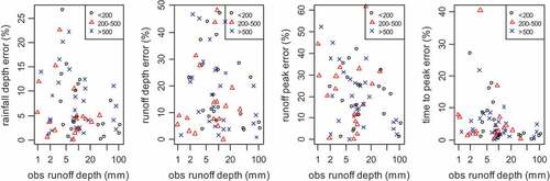
While the rainfall–runoff model fitted slightly better with the larger catchments, it is not clear whether catchment size plays any role in the changes of the performance statistics as a result of the different versions of rainfall, as catchments 7 (553 km²) and 9 (109 km²) exhibit the worst degradation in the performance statistics. This is supported by Figure 12, where the errors split into three classes of catchment area did not display any trend as the class points are very well mixed. Perhaps the result would be much clearer if catchments of sizes below 50 km² were included in the analysis. However, the presented methodology captures the basic spatial and temporal properties of rainfall very well. It is noted that the runoff response of smaller scale catchments is dominated by rainfall variability, whereas for larger scale catchments rainfall volume and the river network aggregation of flows are the overriding factors (e.g. Mandapaka et al. 2009).

5 Summary and concluding remarks

Hydrologists and water engineers are quite often confronted with modelling of catchments having no or a limited number of raingauges located within them. Moreover, the sub-daily modelling time scale makes the long records of daily rainfall data not directly useful. This paper proposes a methodology that uses the available point daily rainfall data on a larger region encompassing the catchment of interest to develop daily rainfields at 1-km² grid scale. The daily rainfield generation model was based on ordinary kriging interpolation. An established relationship between raingauge and radar correlograms for the region was used to infer the appropriate spatial structure for a given day. Raingauge data were replaced with collocated radar data, which were used to simulate the hourly rainfields. A joint sequential simulation of multi-Gaussian fields methodology was employed to simulate radar-like daily rainfields conditioned on the observed point daily records of the day. Options for obtaining the pixel-wise hourly proportions were presented, and multiplication with the pixel-wise daily amounts yielded hourly rainfields.

Sixty-seven storm events from seven nested catchments (93–2513 km²) within the 3088-km² Logan catchment, Queensland, Australia, that had no missing radar rainfall and discharge data were studied. A GIS-based distributed rainfall–runoff model was used to generate and transport runoff to the catchment outlet. The rainfall–runoff model parameters were calibrated by minimizing the sum of square deviations between the observed and simulated hydrographs using the complete radar data. Four performance statistics were used to evaluate simulated hydrographs. With the calibrated parameters, hydrographs were generated using six different rainfall versions, which are combinations of the complete radar pixel-wise daily amounts and hourly proportions, and the simulated ones. Hydrographs from the complete radar data were considered as the true hydrographs, and the degradation in the performance statistics as a result of using the simulated rainfields was used to identify rainfall error propagation to runoff error as a result of the uncertainties relating to pixel-wise proportional assignment only, daily rainfields only, and a combination of both.

Analysis of spatial rainfall variability statistics indicated that the events used in the analysis exhibit significant differences in their spatial structure. Therefore, the performance statistics were averaged over the events within each observed runoff depth class to remove the influence of a particular spatial structure.

The following conclusions can be drawn from the study:

• There is a great difficulty for interpolation methods to capture narrow bands of supercells in regions without raingauges, and the value of a dense gauge network cannot be overstated.

• Assigning the nearest hourly proportions to the pixels appeared marginally to be better than inverse distance weighting interpolation method with three neighbours.

• Uncertainties in daily rainfield simulation alone reduced NSE by 0.066, with 11.6%, 10.9% and 0.7% increases in runoff depth, peak and time to peak errors, respectively.

• Uncertainties in the best hourly proportional option alone caused a 0.062 reduction in NSE, and increases of 5.8%, 5.5% and 0.8% in runoff depth, peak and time to peak errors, respectively. Therefore, the uncertainties in daily rainfall amount alone caused double the reduction in runoff depth and peak errors compared with those resulting from the uncertainties in hourly proportions alone. In essence, the total daily rainfall amount and duration are more important than the intra-daily distribution of rainfall intensities on the statistics of the simulated runoff (Müller-Thomy et al. 2018, Sikorska et al. 2018).

• Degradations caused by the combined uncertainties in the daily rainfield amounts and hourly proportions in the performance statistics were less than the addition of the separate sources alone; only 0.076 reduction in NSE, 9.7% increase in runoff depth error, 9.8% increase in runoff peak error and 1.7% increase in runoff time to peak. However, the degradation values decreased with increasing observed runoff depth.

• Runoff depth and peak errors are on average 1.5 times the error in rainfall depth, which is close to nearly double as identified by Sharif et al. (2002).

• Since catchments analysed were greater than 90 km² in area, there was no evidence that catchment size plays a role in the changes in the performance statistics as a result of the different versions of rainfall. However, the rainfall–runoff model fitted better with the data from the larger catchments.

The methodology presented allows quantification of errors in runoff as a result of the uncertainties in simulated rainfields, isolating all other errors in the runoff generation and transport. Although the quality of the radar rainfall may have some impact on the results, the methodology has a wider implication for comparing alternatives of rainfall input into hydrological models. However, there are limitations from the simplicity of the rainfall–runoff model, and the assumption of uniform model parameters over the catchment. It is expected that spatially fully distributed models will perform better in showing the impacts of spatial rainfall heterogeneity compared with lumped or semi-distributed ones. Testing a couple of different types of rainfall–runoff models will lessen the dependence of the results on one model. Future work will consider different spatial structures, and also improve upon the raingauge marginal distributions. It is intended to use the presented modelling approach to perform spatio-temporal disaggregation of the long-term daily rainfall data into hourly rainfields. This will allow proper assessment of the preservation of spatio-temporal higher-order statistics, especially joint statistics of zero/non-zero rainfall, in long time series of gridded rainfall data.

Acknowledgements

Constructive comments by Hannes Müller and an anonymous reviewer that helped improve the paper are gratefully acknowledged.

Disclosure statement

No potential conflict of interest was reported by the author.

Notes

¹ http://www.bom.gov.au/australia/radar/about/calculating_rainfall_accumulations.shtml.

² https://water-monitoring.information.qld.gov.au/.

References

- Berndt, C., Rabiei, E., and Haberlandt, U., 2014. Geostatistical merging of rain gauge and radar data for high temporal resolutions and various station density scenarios. Journal of Hydrology, 508, 88–101. doi:10.1016/j.jhydrol.2013.10.028
- Bivand, B., 2017. rgrass7: interface between grass 7 geographical information system and R. R package version 0.1-10. Available from: https://CRAN.R-project.org/package=rgrass7 [Accessed 10 January 2018].
- Buishand, T.A., 1978. Some remarks on the use of daily rainfall models. Journal of Hydrology, 36, 295–308. doi:10.1016/0022-1694(78)90150-6
- Buytaert, W., et al., 2006. Spatial and temporal rainfall variability in mountainous areas: a case study from the South ecuadorian andes. Journal of Hydrology, 329 (3–4), 413–421. doi:10.1016/j.jhydrol.2006.02.031
- Chin, D.A., 2013. Water-resources engineering: international edition. 3rd. Harlow, England: Pearson Intl.
- Cole, S.J. and Moore, R.J., 2009. Distributed hydrological modelling using weather radar in gauged and ungauged basins. Advances in Water Resources, 32 (7), 1107–1120. doi:10.1016/j.advwatres.2009.01.006
- Cowpertwait, P.S.P., et al., 1996. Stochastic point process modelling of rainfall. Single-site fitting and validation. Journal of Hydrology, 175, 17–46. doi:10.1016/S0022-1694(96)80004-7
- Cressie, N., 1993. Statistics for spatial data. New York: John Wiley and Sons.
- Dimitriadis, P., et al., 2016. Comparative evaluation of 1D and quasi-2D hydraulic models based on benchmark and real-world applications for uncertainty assessment in flood mapping. Journal of Hydrology, 534, 478–492. doi:10.1016/j.jhydrol.2016.01.020
- Dominguez-Mora, R., et al., 2014. Time and spatial synthetic hourly rainfall generation in the Basin of Mexico. International Journal of River Basin Management, 12 (4), 367–375. doi:10.1080/15715124.2013.842574
- Duan, Q., Sorooshian, S., and Gupta, V.K., 1992. Effective and efficient global optimization for conceptual rainfall–runoff models. Water Resources Research, 28 (4), 1015–1031. doi:10.1029/91WR02985
- Emmanuel, I., et al., 2015. Influence of rainfall spatial variability on rainfall–runoff modelling: benefit of a simulation approach? Journal of Hydrology, 531, 337–348. doi:10.1016/j.jhydrol.2015.04.058
- Gagnon, P., et al., 2002. Spatial disaggregation of mean areal rainfall using gibbs sampling. Journal of Hydrometeorology, 13, 324–337. doi:10.1175/JHM-D-11-034.1
- Glasbey, C.A., Cooper, G., and McGechan, M.B., 1995. Disaggregation of daily rainfall by conditional simulation from a point-process model. Journal of Hydrology, 165, 1–9. doi:10.1016/0022-1694(94)02598-6
- Gómez-Hernández, J.J. and Journel, A.G., 1993. Joint sequential simulation of multi-Gaussian fields. In: A. Soares, ed. Geostatistics Troía ’92. Switzerland: Springer Nature, Vol. 1, 85–94.
- Groisman, P.Y., et al., 1999. Changes in the probability of heavy precipitation: important indicators of climatic change. Climate Change, 42, 243–283. doi:10.1023/A:1005432803188
- Gyasi-Agyei, Y., 2005. Stochastic disaggregation of daily rainfall into one-hour time scale. Journal of Hydrology, 309, 178–190. doi:10.1016/j.jhydrol.2004.11.018
- Gyasi-Agyei, Y., 2011. Copula-based daily rainfall disaggregation model. Water Resources Research, 47, 7. doi:10.1029/2011WR010519
- Gyasi-Agyei, Y., 2012. Use of observed scaled daily storm profiles in a copula based rainfall disaggregation model. Advances in Water Resources, 45, 26–36. doi:10.1016/j.advwatres.2011.11.003
- Gyasi-Agyei, Y., 2013. Evaluation of the effects of temperature changes on fine timescale rainfall. Water Resources Research, 49 (7), 4379–4398. doi:10.1002/wrcr.20369
- Gyasi-Agyei, Y., 2016. Assessment of radar based locally varying anisotropy on daily rainfall interpolation. Hydrological Sciences Journal, 61 (10), 1890–1902. doi:10.1080/02626667.2015.1083652
- Gyasi-Agyei, Y., 2018. Realistic sampling of anisotropic correlogram parameters for daily rainfall interpolation. Journal of Hydrology, 556, 1064–1077. doi:10.1016/j.jhydrol.2016.10.014
- Gyasi-Agyei, Y. and Pegram, G., 2014. Interpolation of daily rainfall networks using simulated radar fields for realistic hydrological modelling of spatial rain field ensembles. Journal of Hydrology, 519, 777–791. doi:10.1016/j.jhydrol.2014.08.006
- Haberlandt, U. and Kite, G.W., 1998. Estimation of daily space-time precipitation series for macroscale hydrological modelling. Hydrological Processes, 12 (9), 1419–1432. doi:10.1002/(ISSN)1099-1085
- Hanson, L.S. and Vogel, R. 2008. The probability distribution of daily rainfall in the United States. In: R.W. Babcock and R.W. Walton, eds., Proceedings of the world environment and water resources congress, 12–16 May. Honolulu, Hawaii, USAReston, VA: American Society of Civil Engineers.
- Koutsoyiannis, D., Onof, C., and Wheater, H.S., 2003. Multivariate rainfall disaggregation at a fine timescale. Water Resources Research, 39 (7), 1173. doi:10.1029/2002WR001600
- Koutsoyiannis, D., Paschalis, A., and Theodoratos, N., 2011. Two-dimensional Hurst-Kolmogorov process and its application to rainfall fields. Journal of Hydrology, 398 (1–2), 91–100. doi:10.1016/j.jhydrol.2010.12.012
- Li, X., et al., 2018. Three resampling approaches based on method of fragments for daily-to-subdaily precipitation disaggregation. International Journal of Climatology, 38 (Suppl.1), e1119–e1138. doi:10.1002/joc.5438
- Mandapaka, P.V., et al., 2009. Dissecting the effect of rainfall variability on the statistical structure of peak flows. Advances in Water Resources, 32, 1508–1525. doi:10.1016/j.advwatres.2009.07.005
- Merz, R. and Blöschl, G., 2003. A process typology of regional floods. Water Resources Research, 39 (12), 1340. doi:10.1029/2002WR001952
- Moussa, R., 1996. Analytical Hayami solution for the diffusive wave flood routing problem with lateral inflow. Hydrological Processes, 10, 1209–1227. doi:10.1002/(ISSN)1099-1085
- Müller-Thomy, H., Wallner, M., and Förster, K., 2018. Rainfall disaggregation for hydrological modeling: is there a need for spatial consistence? Hydrology and Earth System Sciences, 22, 5259–5280. doi:10.5194/hess-22-5259-2018
- Nandakumar, N. and Mein, R.G., 1997. Uncertainty in rainfall–runoff model simulations and the implications for predicting the hydrologic effects of land use change. Journal of Hydrology, 192 (1–4), 211–232. doi:10.1016/S0022-1694(96)03106-X
- Olsson, J., 2006. Spatio-temporal precipitation error propagation in runoff modelling: a case study in central Sweden. Natural Hazards and Earth System Sciences, 6, 597–609. doi:10.5194/nhess-6-597-2006
- Pebesma, E.J., 2004. Multivariable geostatistics in S: the gstat package. Computers & Geosciences, 30, 683–691. doi:10.1016/j.cageo.2004.03.012
- Peel, M.C., Finlayson, B.L., and McMahon, T.A., 2007. Updated world map of the Köppen-Geiger climate classification. Hydrology and Earth System Sciences, 11 (5), 1633–1644. doi:10.5194/hess-11-1633-2007
- Philip, J.R., 1957. The theory of infiltration: 4. Sorptivity and algebraic infiltration equations. Soil Science, 84, 257–264. doi:10.1097/00010694-195709000-00010
- Pui, A., et al., 2012. A comparison of alternatives for daily to sub-daily rainfall disaggregation. Journal of Hydrology, 470, 138–157. doi:10.1016/j.jhydrol.2012.08.041
- Renard, B., et al., 2010. Understanding predictive uncertainty in hydrologic modeling: the challenge of identifying input and structural errors. Water Resources Research, 46, W05521. doi:10.1029/2009WR008328
- Rigby, R.A. and Stasinopoulos, D.M., 2004. Smooth centile curves for skew and kurtotic data modelled using the Box-Cox power exponential distribution. Statistics in Medicine, 23 (19), 3053–3076. doi:10.1002/sim.1861
- Schumm, S.A., 1956. Evolution of drainage systems and slope in badlands at perth Amboy, New Jersey. Bulletin of the Geological Society of America, 67, 597–646. doi:10.1130/0016-7606(1956)67[597:EODSAS]2.0.CO;2
- Segond, M.L., Wheater, H.S., and Onof, C., 2007. The significance of spatial rainfall representation for flood runoff estimation: a numerical evaluation based on the Lee catchment, UK. Journal of Hydrology, 347 (1–2), 116–131. doi:10.1016/j.jhydrol.2007.09.040
- Shah, S.M.S., O’Connell, P.E., and Hosking, J.R.M., 1996. Modelling the effects of spatial variability in rainfall on catchment response. 2. Experiments with distributed and lumped models. Journal of Hydrology, 175 (1–4), 89–111. doi:10.1016/S0022-1694(96)80007-2
- Sharif, H.O., et al., 2002. Numerical simulations of radar rainfall error propagation. Water Resources Research, 38, 8. doi:10.1029/2001WR000525
- Shoji, T. and Kitaura, H., 2006. Statistical and geostatistical analysis of rainfall in central Japan. Computers & Geosciences, 32, 1007–1024. doi:10.1016/j.cageo.2004.12.012
- Sikorska, A.E., Viviroli, D., and Seibert, J., 2018. Effective precipitation duration for runoff peaks based on catchment modelling. Journal of Hydrology, 556, 510–522. doi:10.1016/j.jhydrol.2017.11.028
- Skøien, J.O., et al., 2014. Rtop: an R package for interpolation of data with a variable spatial support, with an example from river networks. Computers & Geosciences, 67, 180–190. doi:10.1016/j.cageo.2014.02.009
- Stasinopoulos, D.M. and Rigby, R.A., 2007. Generalized additive models for location scale and shape (GAMLSS) in R. Journal of Statistical Software, 23 (7). doi:10.18637/jss.v023.i07
- Tarolli, M., et al., 2013. Rainfall space–time organization and orographic control on flash flood response: the Weisseritz event of August 13, 2002. Journal of Hydrologic Engineering, 18 (2), 183–193. doi:10.1061/(ASCE)HE.1943-5584.0000569
- Velasco-Forero, C.A., et al., 2009. A non-parametric automatic blending methodology to estimate rainfall fields from rain gauge and radar data. Advances in Water Resources, 32, 986–1002. doi:10.1016/j.advwatres.2008.10.004
- Viglione, A., et al., 2010. Generalised synthesis of space-time variability in flood response: 1. Analytical framework. Journal of Hydrology, 394 (1–2), 198–212. doi:10.1016/j.jhydrol.2010.05.047
- Westra, S., et al., 2012. Continuous rainfall simulation: 1. A regionalized subdaily disaggregation approach. Water Resources Research, 48 (1), W01535. doi:10.29/2011WR010489
- Wilks, D.S., 1998. Multi-site generalization of a daily stochastic precipitation model. Journal of Hydrology, 210, 178–191. doi:10.1016/S0022-1694(98)00186-3
- Woods, R. and Sivapalan, M., 1999. A synthesis of space-time variability in storm response: rainfall, runoff generation, and routing. Water Resources Research, 35 (8), 2469–2485. doi:10.1029/1999WR900014
- Yao, T. and Journel, A.G., 1998. Automatic modeling of (cross) covariance tables using fast Fourier transform. Mathematical Geology, 30 (6), 589–615. doi:10.1023/A:1022335100486
- Zanon, F., et al., 2010. Hydrological analysis of a flash flood across a climatic and geologic gradient the September 18, 2007 event in Western Slovenia. Journal of Hydrology, 394 (1–2), 182–197. doi:10.1016/j.jhydrol.2010.08.020
- Zoccatelli, D., et al., 2015. The relative role of hillslope and river network routing in the hydrologic response to spatially variable rainfall fields. Journal of Hydrology, 531, 349–359. doi:10.1016/j.jhydrol.2015.08.014
- Zoccatelli, D., et al., 2010. Which rainfall spatial information for flash flood response modelling? A numerical investigation based on data from the Carphatian range, Romania. Journal of Hydrology, 394 (1–2), 148–161. doi:10.1016/j.jhydrol.2010.07.019