Temporal and spatial changes of blue water and green water in the Taihang Mountain Region, China, in the past 60 years

ABSTRACT

Appropriate allocation of limited freshwater resources to humans and ecosystems is an important issue hampering sustainable development in mountainous regions. The Taihang Mountain Region (TMR), including the Yellow and Hai river basins, is an important water source area for the North China Plain. The distributed hydrological model Water and Energy transfer Processes in Large river basins (WEP-L) was used to simulate the water cycle processes and to summarize the temporal and spatial changes in the blue and green water in the TMR from 1956 to 2015. The results show that in the period 2011–2015 the annual average blue water decreased by 7.31 × 10⁹ m³, while the annual average green water increased by 13.60 × 10⁹ m³ compared to 1956–1960. At the inter-annual time scale, the blue water exhibited a downward trend while the green water exhibited an upward trend. The amount of seasonal blue water in the TMR is ranked in descending order: summer, autumn, spring and winter, while for green water, the rank is summer, spring, autumn and winter. The amounts of blue and green water are higher on the windward than on the leeward slopes. The blue water yield is generally higher in forests and grasslands than in farmland, while the green water exhibits the opposite response. A greater emphasis should be placed on the widening gap between blue water and green water due to climate warming, and on soil and water conservation measures.

KEYWORDS:

• Taihang Mountain Region
• blue water
• green water
• competitive water use
• temporal and spatial distribution

Editor A. Castellarin; Guest Editor Y. Chen

1 Introduction

Renewable freshwater is indispensable and crucial for the socio-economic system and the Earth’s ecosystems (Postel et al. 1996, Vörösmarty et al. 2000, 2010). However，only 2.5% of the Earth’s water is freshwater, most of it stored in glaciers or deep groundwater; thus, only a relatively small amount can be easily utilized (Oki and Kanae 2006). With the growing demands of the population and ecosystems for freshwater, the appropriate allocation of limited water resources to ensure sustainable development at the maximum level is one of the most important issues that cannot be ignored.

Land-use/land-cover patterns in mountainous areas have important impacts on the water resource regulation and allocation. On the one hand, mountainous areas are key water sources for the plains areas and provide valuable freshwater sources for cities where most of the water is consumed. On the other hand, mountainous areas with high vegetation cover are natural ecological barriers and are, for the most part, responsible for regulating the climate (increasing air humidity, absorbing CO₂, water conservation, etc.), maintaining biodiversity, supplying ecological products, and for many other functions. However, land-use/land-cover changes in mountainous areas represent a double-edged sword for water resources regulation. Although a greater vegetation cover enhances the ecological value, the increase in freshwater consumption results in a decrease in the available water crucial to human society. In contrast, vegetation removal increases the available runoff and results in a series of adverse effects, such as soil erosion, reduction in ecological diversity and degradation of ecosystems. Therefore, certain questions need to be addressed. What drives the changes in the water cycle in mountainous regions under the influence of climate change and human activities? What impact will these changes have on the coordinated development of regional economies and ecosystems? In view of the above questions, research focusing on competitive water use in mountainous areas is still required.

Based on the concept proposed by the Swedish scientist Malin Falkenmark (Falkenmark 1997), freshwater resources may be classified as green water or blue water. The former is crucial for sustaining ecosystems and crop production, while the latter supports socio-economic development. This concept systematically integrates the water cycle processes and human activities (Falkenmark 1999), and has constantly been improved upon (Rockström 1999, Falkenmark and Rockström 2006, Falkenmark et al. 2009, Falkenmark and Rockström 2010); the basic meaning behind the concept has been extensively accepted, with notable progress.

Green water has been studied at the global scale (Gerten et al. 2005, Yang and Zehnder 2007, Hoff et al. 2010, Mekonnen and Hoekstra 2010), the watershed scale (Sun and Ren 2013, Zhang et al. 2014), and areas of several square kilometres (Liu et al. 2009, Glavan et al. 2013). Other studies have been conducted on the assessment of blue and green water (Schuol et al. 2008), and the distribution of blue and green water (Zuo et al. 2015). Some scholars (Abbaspour et al. 2009, Xu 2013, Zang et al. 2015) have studied the impacts of climate change, and land-use/land-cover change (LUCC) on changes in blue and green water. The consumption of blue and green water in grain production (Rost et al. 2008, Liu and Yang 2010) and the blue and green water footprint (Siebert and Döll 2010, Zhuo et al. 2016) are also the focus of intense research, as are studies on water security (Schmitz et al. 2013, Veettil and Mishra 2016). The research tools include the simple water balance model, the global crop water model (GCWM) (Siebert and Döll 2008), the GIS-based environmental policy integrated climate model (GEPIC) (Liu et al. 2007a), the process-based dynamic global vegetation and water balance model, Lund-Potsdam-Jena (LPJ; Rost et al. 2008), and the Soil and Water Assessment Tool (SWAT; Arnold and Allen 1996). Although significant progress has been made, there is still a lack of research on the changes in blue and green water and on the water conflict between humans and ecosystems in mountainous areas.

China is a mountainous country, with 69% of its land comprising mountains, hills and highlands. In addition, China faces severe water shortages, with a per capita water resource of 2200 m³, which represents one-quarter of the worlds’ average (Liu et al. 2007b). Several important cities, such as Beijing, Tianjin and Shijiazhuang, are located in the North China Plain. However, the per capita water resource of these cities is 501 m³ (Xia et al. 2007), less than one-quarter of the national average (i.e. 1/16th of the world’s average). The critical shortage of water resources has aggravated the water conflict between humans and ecosystems, resulting in a series of ecological and environmental problems, including drying up of rivers, ecological degradation and groundwater recession in the North China Plain (Xia et al. 2004).

The Taihang Mountain region (TMR), also called the “water tower” of the North China Plain, is situated in the transitional zone of the North China Plain and the Loess Plateau. In recent decades, the water cycle in the Taihang Mountains has undergone a series of changes due to climate change (temperature increase and precipitation decrease) and human activities (urban expansion and vegetation rehabilitation) (Xu 2013, Feng et al. 2016). The quantitative assessment of freshwater allocation and its spatio-temporal changes with regard to humans and ecosystems can provide not only a scientific basis for coordinated development in the TMR, but also useful information for other similar mountainous regions worldwide.

In order to describe in detail the competitive water use by humans and ecosystems, it is necessary to limit the concept of green water to a certain extent. In this study, blue water is defined as river runoff and green water is defined as the evapotranspiration (ET) from the vegetation to the atmosphere (i.e. rainwater used efficiently by the vegetation). Physically-based, distributed hydrological models (PBDHM), which have the advantage of a better description of the mechanisms of hydrological and land surface processes, are regarded as a powerful tool for analysing the water conflict between the two systems, as well as for assessing the blue and green water spatio-temporally. During recent years, PBDHMs have been developed rapidly due to advances in techniques in geographic information systems (GIS), remote sensing (RS) and global positioning systems (GPS). Several representative models have been proposed, such as the VIC model (Liang et al. 1994), the WetSpa model (Wang et al. 1996), the geomorphology-based hydrological model (GBHM; Yang et al. 1998), the distributed time-variant gain model (DTVGM; Xia et al. 2005), the Water and Energy transfer Processes in Large river basins (WEP-L; Jia et al. 2006) and the Liuxihe model (Chen et al. 2011). The WEP-L model, in which contour bands are used to describe the effects of topography in large basins, is well suited to represent the vertical characteristics of the water cycle processes in mountainous areas. Therefore, we employed the WEP-L model in this study.

In this study, we simulated the hydrological processes in the TMR from 1956 to 2015 and summarized the temporal and spatial evolution of the blue water and green water. The highlights of this study are the following:

(1) The physically-based distributed hydrological model WEP-L is used and validated for water cycle simulations in the TMR to assess the amounts of blue water and green water, and to determine the changes in blue water and green water in the past 60 years.

(2) The inter-annual, seasonal and spatial changes in precipitation, blue water and green water in the past six decades, including the change trends and abrupt change points, are studied. Moreover, the water cycle differences between windward slope and leeward slope are revealed.

(3) To validate the green water processes, MODIS vegetation index data and ET products derived from remote sensing data are used, and a time series analysis is conducted.

2 Study area and methods

2.1 Study area

The TMR (127 800 km²) (Figs 1 and 2) is located at the eastern margin of the second step of China’s terrain and is regarded as the eastern boundary of the Loess Plateau, with the Shanxi Plateau to the west and the North China Plain to the east. The TMR stretches over 400 km from the Xishan Mountains of Beijing in the north to the Wangwu Mountains in the transboundary region of Henan and Shanxi provinces in the south. The area is situated in the transitional zone between a semi-humid and a semi-arid region, and extends from 34°36′N, 110°10′E to 40°47′N, 116°35′E. It spreads across the four provincial administrative units of Beijing, Hebei, Shanxi and Henan and contains two first-class water resources regions, the Haihe River Basin Part (HRBP) (86 500 km²) and the Yellow River Basin Part (YRBP) (41 300 km²). The main vegetation type of the eastern part near the North China Plain consists of broad-leaved deciduous forest, while the western part near the Loess Plateau consists of a forest-steppe zone and a steppe zone.

Figure 1. Location of the study area: (a) details of the Taihang Mountain Region (TMR) showing the Yellow and Haihe river basin parts, and (b) the sub-basins studied and the selected meteorological and hydrological stations.

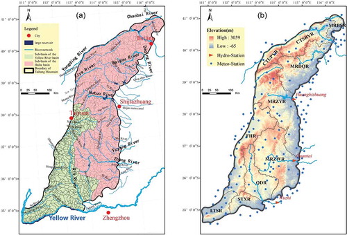
Figure 2. Land cover in the TMR in (a) 1980, (b) 1995, (c) 2005 and (d) 2010.

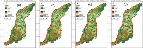
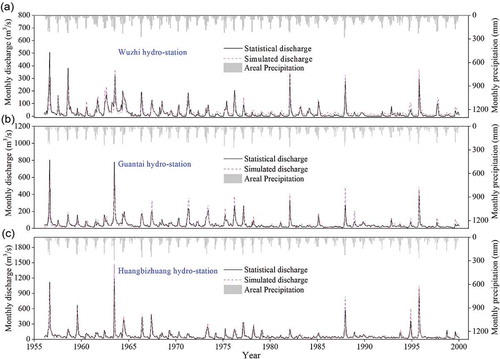
Figure 3. Verification of simulated monthly discharges at (a) Wuzhi station, (b) Guantai station and (c) Huangbizhuang station.

The TMR has a temperate monsoon climate. The southeast monsoon brings warm moist air flows supplied by the Pacific; therefore, the summer in this area is hot and rainy. The winter is cold and dry because of the Siberian cold current from the northwest direction. The annual average precipitation ranges from 400 to 600 mm, with uneven distribution throughout the year.

The main river systems from north to south are: the Yellow River stem and its tributaries – the Qin and Dan rivers; and the Haihe River tributaries – the Chaobai, Yongding, Daqing, Hutuo, Fuyang and Zhang rivers.

2.2 Data description

The digital elevation model (DEM) data was obtained from the Consultative Group for International Agricultural Research-Consortium for Spatial Information (CGIAR-CSI) Shuttle Radar Topography Mission (SRTM) 90-m DEM database (http://srtm.csi.cgiar.org/). The measured daily meteorological data from 1956 to 2015, including precipitation, air temperature, relative humidity, wind velocity and sunshine duration, were obtained from the National Meteorological Science Data Sharing Service Platform (http://data.cma.cn), which has 164 stations.

The land-use and land-cover data for 1980, 1995, 2005, 2010 and 2014 were derived from the data center for Resources and Environmental Sciences, Chinese Academy of Sciences (RESDC) (http://www.resdc.cn). The soil data were obtained from the second national general soil survey with a resolution of 1:100 000. The monthly maximum MODIS normalized difference vegetation index (NDVI) datasets, with a spatial resolution of 500 m, from 2000 to 2015 were provided by the geospatial data cloud site at the Computer Network Information Center of the Chinese Academy of Sciences (http://www.gscloud.cn). The global 8 km × 8 km ET datasets derived from remote sensing data were provided by the Numerical Terradynamic Simulation Group at the University of Montana, USA (http://www.ntsg.umt.edu/project/global-et.php). For more details on the ET data products, one may refer to the literature (Zhang et al. 2009, 2010, 2015). The statistical discharge (i.e. the naturalized river discharge) series were derived from the monitoring data of the hydrological stations and the statistics of the water consumption related to rivers and reservoirs.

2.3 WEP-L model

The WEP-L model was developed based on the WEP model (Water and Energy transfer Processes) (Jia et al. 2001) for water cycle simulations in large-scale basins. To ensure the rapidity and accuracy of the overall hydrological process simulations, the advantages of the water cycle hydrological model and land surface model – the Soil–Vegetation–Atmosphere Transfer System (SVATS) model – are integrated into the model for the coupled water cycle–energy transfer simulations. The varying source area (VSA) theory is integrated for a dynamic simulation of surface water, groundwater and soil water.

The WEP-L model uses elevation contours in the sub-basins as its basic calculation unit and different time steps as the calculation interval. The model is suitable for fine-scale simulations of water cycle processes, and has great potential for water resources assessment under various meteorological and underlying surface conditions, due to its physical foundation of the hydrological and eco-hydrological mechanisms and the flexibility of using parameters based on the characteristics of the study area. The WEP-L model has been applied successfully in several basins (Jia et al. 2005, 2009, 2012).

The soil and water conservation measures in the TMR mainly include increases in the vegetation cover (afforestation of the wasteland, planting of grass), terracing of sloping land and the construction of silting dams. Based on land-use data of different phases, the WEP-L model uses a linear interpolation to obtain land-use information for each year to describe inter-annual changes in the land use/land cover. The model divides the land use/land cover into five groups: water bodies, impervious areas, soil–vegetation, irrigated farmland and non-irrigated farmland. The leaf area index (LAI), vegetation fraction (VEG), depression storage depth and the Manning roughness of the five subgroups are determined and calibrated separately. In this sense, the impacts of the increases in vegetation cover and the terracing of sloping land on the runoff generation and flow can be characterized.

In the model, it is assumed that the silting dams have functions that are similar to those of reservoirs, and the following procedure is carried out:

Step 1. Based on the survey and information provided by the water authorities, information on the location and storage capacity of a silting dam is obtained; then the upper critical threshold of the storage capacity of a silting dam is determined for each contour band.

Step 2. If and only if the inflow exceeds the given threshold, the excess water can flow out and the discharge routing can be computed.

Step 3. The upper threshold parameter of the storage capacity is calibrated similarly to the other parameters (e.g. depression storage depth and Manning roughness) to improve the accuracy of the model simulation.

The Nash-Sutcliffe efficiency coefficient (NSE; Nash and Sutcliffe 1970) and the percent bias (PBIAS; Gupta et al. 1999) are used to evaluate the model performance. The equations for the two coefficients are expressed as follows:

(1) $\mathrm{N}\mathrm{S}\mathrm{E}=1-\frac{\sum _{i=1}^n{(Q_{\mathrm{o}\mathrm{b}\mathrm{s}}^i-Q_{\mathrm{s}\mathrm{i}\mathrm{m}}^i)}^2}{\sum _{i=1}^n{(Q_{\mathrm{o}\mathrm{b}\mathrm{s}}^i-\overline{Q_{\mathrm{o}\mathrm{b}\mathrm{s}}})}^2}$(1)

(2) $\mathrm{P}\mathrm{B}\mathrm{I}\mathrm{A}\mathrm{S}=\frac{\sum _{i=1}^n(Q_{\mathrm{o}\mathrm{b}\mathrm{s}}^i-Q_{\mathrm{s}\mathrm{i}\mathrm{m}}^i)}{\sum _{i=1}^n{Q}_{\mathrm{o}\mathrm{b}\mathrm{s}}^i}$(2)

where $O_{\mathrm{o}\mathrm{b}\mathrm{s}}^i$ (m³/s) is the observed runoff, $Q_{\mathrm{s}\mathrm{i}\mathrm{m}}^i$ (m³/s) is the simulated runoff, and $\overline{Q_{\mathrm{o}\mathrm{b}\mathrm{s}}}$ (m³/s) is the average of the observed values.

2.4 Trend test and abrupt change point analysis

In this study, the nonparametric Mann-Kendall test (Kendall 1975), which is widely used to assess the significance of trends in hydro-meteorological time series data and for many other variables (Xu et al. 2003, 2005, Zhang et al. 2008), is used to analyse the change trends of the blue and green water series. The nonparametric Pettitt test (Pettitt 1979), an effective tool to detect the abrupt change point of a time series (Ma et al. 2008, Zuo et al. 2012), is chosen to assess the change points of the precipitation, blue water and green water.

2.5 Sensitivity analysis of blue and green water to climate change

Based on the WEP-L model, eight scenarios (Table 1) are designed for a quantitative analysis of the elastic coefficients of the blue and green water to precipitation and temperature changes. The equations for the elastic coefficients are:

(3) $P_{\mathrm{b}\mathrm{l}\mathrm{u}\mathrm{e}}=\frac{\mathrm{\Delta }{W}_{\mathrm{b}\mathrm{l}\mathrm{u}\mathrm{e}}^{\mathrm{\Delta }\mathrm{p}}/{\bar{W}}_{\mathrm{b}\mathrm{l}\mathrm{u}\mathrm{e}}}{\left|\mathrm{\Delta }p\right|/\bar{p}}$(3)

(4) $P_{\mathrm{g}\mathrm{r}\mathrm{e}\mathrm{e}\mathrm{n}}=\frac{\mathrm{\Delta }{W}_{\mathrm{g}\mathrm{r}\mathrm{e}\mathrm{e}\mathrm{n}}^{\mathrm{\Delta }\mathrm{p}}/{\bar{W}}_{\mathrm{g}\mathrm{r}\mathrm{e}\mathrm{e}\mathrm{n}}}{\left|\mathrm{\Delta }p\right|/\bar{p}}$(4)

(5) $T_{\mathrm{b}\mathrm{l}\mathrm{u}\mathrm{e}}=\frac{\mathrm{\Delta }{W}_{\mathrm{b}\mathrm{l}\mathrm{u}\mathrm{e}}^{\mathrm{\Delta }\mathrm{T}}/{\bar{W}}_{\mathrm{b}\mathrm{l}\mathrm{u}\mathrm{e}}}{\left|\mathrm{\Delta }T\right|/\bar{T}}$(5)

(6) $T_{\mathrm{g}\mathrm{r}\mathrm{e}\mathrm{e}\mathrm{n}}=\frac{\mathrm{\Delta }{W}_{\mathrm{g}\mathrm{r}\mathrm{e}\mathrm{e}\mathrm{n}}^{\mathrm{\Delta }\mathrm{T}}/{\bar{W}}_{\mathrm{g}\mathrm{r}\mathrm{e}\mathrm{e}\mathrm{n}}}{\left|\mathrm{\Delta }T\right|/\bar{T}}$(6)

Table 1. Scenarios for the sensitivity analysis.

Scenario no.	Δp	ΔT
S1	−10%	-
S2	−5%	-
S3	5%	-
S4	10%	-
S5	-	−2°C
S6	-	−1°C
S7	-	1°C
S8	-	2°C

where $\bar{p}$ (mm) and $\bar{T}$ (°C) are the annual average precipitation and temperature from 1956 to 2015; ${\bar{W}}_{\mathrm{b}\mathrm{l}\mathrm{u}\mathrm{e}}$ (mm) is the annual average blue water; ${\bar{W}}_{\mathrm{g}\mathrm{r}\mathrm{e}\mathrm{e}\mathrm{n}}$ (mm) is the annual average green water; $\mathrm{\Delta }p$ (mm) is the precipitation increment by percentage; $\mathrm{\Delta }T$ (°C) is the temperature increment; $\mathrm{\Delta }{W}_{\mathrm{b}\mathrm{l}\mathrm{u}\mathrm{e}}^{\mathrm{\Delta }\mathrm{p}}$ (mm) and $\mathrm{\Delta }{W}_{\mathrm{g}\mathrm{r}\mathrm{e}\mathrm{e}\mathrm{n}}^{\mathrm{\Delta }\mathrm{p}}$ are the blue water and green water increments with $\mathrm{\Delta }p$; $\mathrm{\Delta }{W}_{\mathrm{b}\mathrm{l}\mathrm{u}\mathrm{e}}^{\mathrm{\Delta }\mathrm{T}}$ (mm) and $\mathrm{\Delta }{W}_{\mathrm{g}\mathrm{r}\mathrm{e}\mathrm{e}\mathrm{n}}^{\mathrm{\Delta }\mathrm{T}}$ (mm) are the blue water and green water increments with $\mathrm{\Delta }T$, respectively.

3 Results

3.1 Calibration and performance of the WEP-L model

There is no hydraulic connection between the two catchments in the TMR, hence two distributed hydrological models are established; 1634 sub-basins and 7351 basic calculation units (contours) are set according to the terrain, including 1634 sub-basins and 5096 contours in the Haihe River Basin and 507 sub-basins and 2435 contours in the Yellow River Basin. The division of the sub-basins is shown in Figure 1.

The parameters in the WEP-L model can be divided into three categories (Jia et al. 2001): (a) the soil and aquifer parameters: the saturated soil moisture content, residual soil moisture content, field capacity, moisture–suction relationship, thickness of soil layer and aquifers, saturated hydraulic conductivity, specific yield of the unconfined aquifer, and the relationship between the hydraulic conductivity and the soil moisture; (b) the parameters of runoff yield and flow concentration: the maximum depression storage depth of various surfaces and Manning’s roughness coefficients for the overland flow and the river channel; and (c) the vegetation parameters: the vegetation fraction, LAI, maximum canopy interception depth, root depth, canopy resistance and aerodynamic resistance.

The parameters of the four soils (sand, loam, clay loam and clay) in the TMR are shown in Table 2; the maximum depression storage depths and Manning’s roughness of various land-use types are shown in Table 3; and the vegetation parameters are shown in Table 4. The calibrated parameters include the soil saturated hydraulic conductivity, Manning’s roughness coefficients and the hydraulic conductivity of unconfined aquifers; the remaining parameters are described in the literature (Jia et al. 2001, 2006, 2012).

Table 2. Soil parameters of the TMR main soil types.

Parameter	Sand	Loam	Clay loam	Clay
Thickness of three soil layers (m)	0.20–1.40	0.20–1.40	0.20–1.40	0.20–1.40
Saturated moisture content (%)	0.41	0.46	0.40	0.40
Field capacity (%)	0.17	0.28	0.37	0.39
Residual soil moisture content (%)	0.08	0.12	0.17	0.25
Saturated hydraulic conductivity (m/s)	2.50 × 10^−3	7.00 × 10^−4	2.00 × 10^−4	3.00 × 10^−4
Suction at wet front (cm)	6.1	8.9	12.5	17.5

Table 3. Maximum depression storage depth (MDSM) and Manning’s roughness of overland flow (MROF) in the TMR. IF: irrigated farmland; NIF: no-irrigated farmland; SP: sloping cultivated land; BS: bare soil; UA: urban area; WB: water body.

Land-use type	Forest	Grassland	Paddy	IF	NIF	SP	BS	UA	WB
MDSD (mm)	6–20	3–13	10–15	8–10	8–12	1.5–4	1–3	2	0
MROF (mm)	0.3	0.1	0.2	0.2	0.2	0.1	0.05	0.02	0.01

Table 4. Vegetation parameters in the TMR.

Parameter	Maximum	Minimum	Average
Vegetation fraction	0.80	0.20	0.48
Leaf area index, LAI	2.85	0.08	1.105

The criteria for the model calibration and verification are to maximize the NSE of the simulated and statistical monthly average discharge and to minimize the absolute value of the PBIAS. The calibration of the WEP-L model is performed using the “trial and error” approach; the parameters are adjusted until the simulated hydrological processes cannot be further improved. The results are shown in Table 5.

Table 5. Performance of the WEP-L model in the TMR in calibration and validation periods. NSE: Nash-Sutcliffe efficiency criterion; PBIAS (%): percent bias.

Period	Station	River	NSE	PBIAS
Calibration (1956–1979)	Wuzhi	Qin	0.75	5.90
	Guantai	Zhang	0.79	−5.62
	Huangbizhuang	Hutuo	0.82	−3.06
Validation (1980–2000)	Wuzhi	Qin	0.68	4.91
	Guantai	Zhang	0.73	9.86
	Hubizhuang	Hutuo	0.75	5.02

Because only runoff data for three hydro-stations (located on the three major tributaries in the TMR) from 1956 to 2000 are available, the model calibration and verification are performed for the corresponding sub-basins of the Wuzhi station (located on the Qin River stem), Guantai station (located on the Zhang River stem) and Huangbizhuang station (located on the Hutuo River stem).The monthly runoff data simulated by the WEP-L model are validated by statistical runoff data. The results indicate a good accuracy of the model simulation, with PBIAS of less than 10% and NSE greater than 0.7 (see Table 5, Fig. 3).

3.2 Quantitative assessment of blue water and green water

Table 6 shows the average annual amounts of annual precipitation, green water and blue water in the TMR for the period 1956–2015. The average annual precipitation in the whole TMR is 549.36 mm, while the average annual green water is 143.07 mm, which is 1.55 times bigger than that of the blue water (92.47 mm). In the YRBP (western TMR), the average annual precipitation, blue water and green water are 567.93, 74.26 and 161.49 mm, respectively, while in the HRBP (eastern TMR), the corresponding values are 540.49, 101.17 and 134.28 mm, respectively (Table 6).

Table 6. Average annual precipitation, blue water and green water at the sub-basin and basin level in the TMR for the period 1956–2015.

Sub-basin*	Precipitation (mm)	Blue water (mm)	Green water (mm)
FHR	515.95	57.48	137.64
LTSR	566.86	82.14	238.18
STXR	643.25	99.81	213.49
QDR	607.41	82.30	132.76
MRBSR	566.05	106.05	136.25
CTSRYR	435.15	60.05	147.31
CTURYR	441.44	78.23	124.40
MRDQR	563.15	130.77	130.56
MRZYR	542.24	107.75	123.04
MRZWR	584.49	95.35	144.23
YRBP	567.93	74.26	161.49
HRBP	540.49	101.17	134.28
TMR	549.36	92.47	143.07

* see Figure 1.

According to the northeast-to-southwest direction of the TMR (Fig. 1), the sub-basins CTUPYR, CTSRYR and FHR (Fig. 1) are located on leeward slopes, while the remaining seven sub-basins are located on windward slopes. It is observed that the precipitation and the blue water amounts are lower on the leeward slopes than on the windward slopes. Moreover, the amount of blue water and precipitation is generally higher in the HRBP than in the YRBP.

The inter-decadal variation in precipitation, temperature, blue water and green water in the TMR is shown in Table 7. Generally speaking, the precipitation has decreased, the temperature has risen, the blue water has decreased, and the green water has increased over the past 60 years. However, the changes in the four variables are not strictly consistent. The temperature has an increasing trend for the entire period, while the precipitation exhibits a decreasing trend prior to 2000 and an increasing trend in 2000–2015.

Table 7. Changes in precipitation, temperature, blue water and green water in the TMR in the past six decades.

Period	Precipitation (mm)	Temperature (ºC)	Blue water (mm)	Green water (mm)	Ratio (green/blue)
1956–1960	620.12	9.70	130.51	116.75	0.89
1961–1970	592.12	9.75	117.09	117.46	1.00
1971–1980	548.39	9.88	91.77	133.33	1.45
1981–1990	535.54	10.01	83.44	133.60	1.60
1991–2000	511.84	10.58	87.41	111.88	1.28
2001–2010	520.67	10.90	73.22	192.20	2.62
2011–2015	555.08	10.89	73.28	223.19	3.05
1956–2015	549.36	10.24	92.47	143.07	1.55

During the six decades, the blue water has decreased by about half (from 130.51 to 73.28 mm), while the green water has doubled (from 116.75 to 223.19 mm). The ratio of green water to blue water in (Table 7, last column) indicates that the amount of green water was lower in the 1970s, after which its amount was higher.

Based on the temporal changes in precipitation, temperature, blue water and green water, it is suggested that there are strong relationships between blue water and precipitation, as well as between green water and temperature.

3.3 Annual changes in the blue water and green water

The annual changes in precipitation, blue water and green water are also evaluated. As shown in Figure 4(a), the amount of blue water in the TMR ranges from 50.77 to 248.03 mm and the amount of green water from 82.76 to 234.25 mm. Figure 4(b) and (c) shows the data for the YRBP and HRBP, respectively. The WEP-L model divides the river runoff (blue water in this study) into surface runoff, interflow and groundwater, and, by definition, the groundwater is part of the blue water. Therefore we analysed the proportion of groundwater in the blue water in the TMR. Between 1956 and 2015, the ratios of groundwater to blue water in the TMR, YRBP and HRBP were 59%, 52% and 62%, respectively.

Figure 4. Annual blue water and green water in (a) the whole TMR, (b) the YRBP and (c) the HRBP (see Fig. 1(b) for locations).

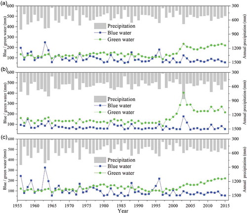
In general, three observations can be made at the inter-annual scale: (1) the blue water decreases and the green water increases, which is in accordance with the results at the inter-decadal scale; (2) the greater the precipitation, the higher the amount of both blue water and green water; and (3) the fluctuations of the blue water series are stronger than those of the green water.

Specifically, the time series of the blue and green water can be divided into three phases. In the period from 1956 to 1973, there is a small difference between the amounts of blue water and green water. However, in the second period (1974–1997), the amount of green water is generally higher than that of blue water, except for some years with extremely heavy precipitation, such as 1988, 1995 and 1996. Then, after 1997, the amount of green water is clearly higher.

The spatial distribution of blue and green water in the eastern and western TMR is not exactly the same. The blue water has a larger extent in the HRBP, while the green water has a larger extent in the YRBP.

Figure 5 shows the annual changes in blue water and green water at the sub-basin scale in the TMR. The annual average precipitation and the blue water are generally lower on the leeward slopes than on the windward slopes.

Figure 5. Annual blue water and green water in the 10 sub-basins of the TMR: (a)–(d) the YRBP, and (e)–(j) the HRBP (see Fig. 1(b) for sub-basin locations).

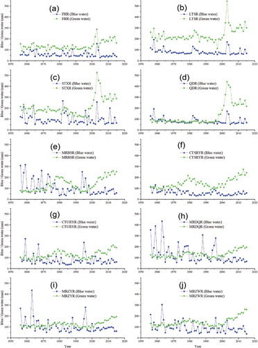
A comparison of the blue water yield for different land-use types (Fig. 2) illustrates that the blue water yield is generally higher in forest and grassland than in farmland, while the distribution of green water is the opposite. For instance, the MRZYR sub-basin is covered mainly by forest and grassland, and the amount of blue water is 107.75 mm, with precipitation of 542.24 mm (Table 6). In contrast, although the precipitation is 584.49 mm, the blue water in the MRZWR sub-basin, with a large proportion of farmland, is only 95.35 mm. The amount of green water in the LTSR and STXR sub-basins is 238.18 and 213.49 mm, respectively, while for the QDR and FHR sub-basins, which have less cultivated land than the former sub-basins, the amount of green water is 137.64 and 132.76 mm, respectively.

This phenomenon is a result of the cultivation measures that are widely adopted to supply sufficient water and soil nutrients for crop production, such as land formation, ridge building, and soil and water conservation measures. All these measures increase the water entrapment due to ET and regional roughness (resulting in less blue water), increase the soil infiltration and soil moisture, and enhance the regional potential ET and integrated ET (resulting in more green water).

3.4 Seasonal changes in blue water and green water

In the TMR, the spring and autumn last for a relatively short period and spring temperatures are higher than autumn temperatures, with less precipitation in spring than in autumn. The seasonal average precipitation and temperatures in the YRBP, HRBP and TMR as a whole, in the period 1956–2015, are shown in Table 8. The seasonal changes in precipitation, blue water and green water in the period 1956–2015 are shown in Figure 6 for the TMR and Figure 7 for the YRBP and HRBP.

Table 8. Seasonal average precipitation and temperature in the recent 60 years (1956–2015) in the TMR.

Basin	Annual	Spring	Summer	Autumn	Winter
Precipitation (mm)
YRBP	567.93	98.79	310.02	138.73	20.39
HRBP	540.49	74.93	348.22	103.76	13.58
TMR	549.36	82.64	335.87	115.06	15.78
Temperature (°C)
YRBP	11.63	12.75	23.61	11.74	−1.59
HRBP	9.57	10.75	22.33	9.74	−4.53
TMR	10.24	11.39	22.74	10.39	−3.58

Figure 6. Seasonal precipitation, blue water and green water in the TMR in (a) spring, (b) summer, (c) autumn and (d) winter.

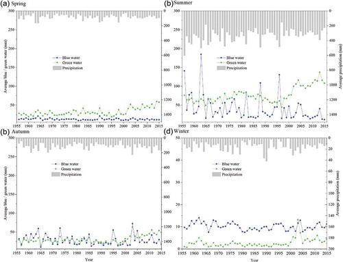
Figure 7. Seasonal blue water and green water in (a) the YRBP in spring, summer and autumn, (b) the YRBP in winter, (c) the HRBP in spring, summer and autumn and (d) the HRBP in winter.

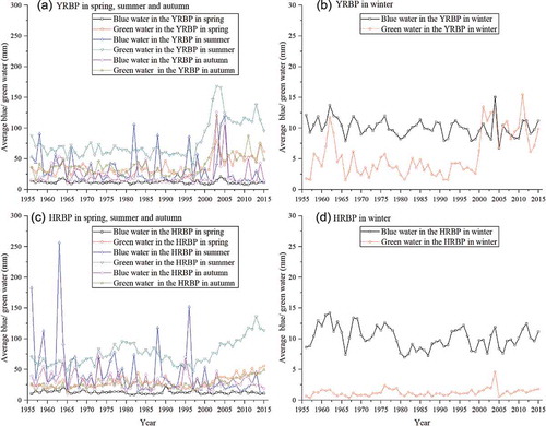
The ranking of the amount of seasonal average blue water in descending order is summer, autumn, spring and winter, and the ranking for the green water is summer, spring, autumn and winter. Apart from some years when the precipitation is excessive, the amount of green water is higher, but the result is opposite in the winter. However, it is worth pointing out that no less than 10% of the blue water and not more than 2% of the green water are produced in the TMR in the winter, and the amount of green water is much lower in the HRBP than in the YRBP in the winter.

Considering the regional cold and dry climate, the relatively low temperature (below 0°C) inhibits water exchange between the soil and the atmosphere and reduces the regional potential evaporation, resulting in less green water. Although there is less precipitation in the winter, the runoff can be recharged by soil water and groundwater. Hence, it is reasonable that the winter precipitation, accounting for 2.87% of the annual average amount, contributes 11.06% of the annual average blue water in the TMR.

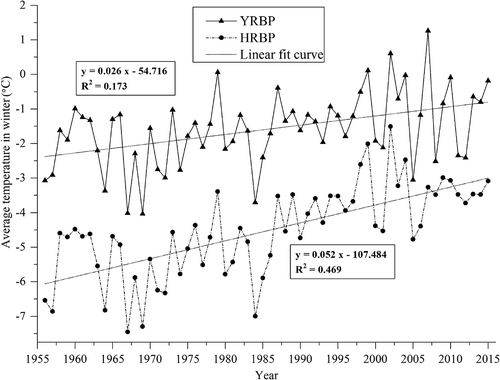
As shown in Figure 8, the trend of the average winter temperatures in the TMR has been increasing over the most recent 60 years. The ascending gradients in the YRBP and HRBP are 0.026 and 0.052°C/year, respectively. In addition, the fact that the average temperature in the HRBP (−4.53°C, located at a higher latitude) is lower than the average temperature in the YRBP (−1.59°C, located at a relatively lower latitude) explains the difference in the amounts of green water in the two regions in the winter.

Figure 8. Average winter air temperature in the YRBP and HRBP.

3.5 Results of change trend and abrupt change analysis

The results of the Mann-Kendall and Pettitt tests are shown in Table 9. A statistically significant downtrend at the p = 0.01 significance level is observed for the annual blue water in the TMR and in eight of the 10 sub-basins. For the entire TMR region, the rate of blue water change is −0.72 mm/year, whereas the values for the 10 sub-basins vary from −1.30 to −0.20 mm/year. There are significant positive trends (α = 0.01) for the annual green water time series: this shows significant positive trends (α = 0.01/0.05) in all of the 10 sub-basins with regard to the slope (0.83–2.37 mm/year). However, the results indicate that the intensity of the blue water in the YRBP is higher, while the intensity of the green water in the HRBP is higher. At the 0.01 significance level, the change points of the blue water time series in the TMR occur in the period 1975–1985, close to the change points of the annual average precipitation, while the change points of the green water occur close to 1997–2001, except for the MRBSR sub-basin.

Table 9. Mann-Kendall and Pettitt test results for precipitation (P), blue water (BW) and green water (GW). P_b: probabilities associated with the Pettitt test. A positive value of slope β means an upward trend and a negative value means a downward trend.

Sub-basin	Variable	Mann-Kendall test			Pettitt test
		Z statistic	Significance	Slope, β (mm/year)	Change point (year)	Pb	Significance
FHR	P	–1.72	-	–1.39	1977	0.527	-
	BW	–2.82	**	–0.27	1985	0.080	-
	GW	3.23	**	0.83	1999	6.8 × 10^−6	**
LTSR	P	–1.06	-	–0.88	1989	0.842	-
	BW	–3.95	**	–0.40	1985	0.014	*
	GW	3.16	*	1.06	2000	1.0 × 10^−5	**
STXR	P	–1.69	-	–1.74	1985	0.477	-
	BW	–1.52	-	–0.43	1985	0.495	-
	GW	1.96	*	1.33	1997	5.6 × 10^−7	**
QDR	P	–1.80	-	–1.53	1977	0.442	-
	BW	–3.97	**	–0.41	1985	0.014	*
	GW	3.73	**	2.08	1997	1.5 × 10^−7	**
MRBSR	P	–1.57	-	–1.45	1979	0.514	-
	BW	–3.05	**	–0.99	1979	0.020	*
	GW	4.31	**	2.37	1972	1.9 × 10^−4	**
CTSRYR	P	–0.93	-	–0.60	2006	0.746	-
	BW	–3.57	**	–0.51	1979	3.7 × 10^−4	**
	GW	5.36	**	1.70	2002	5.5 × 10^−4	**
CTURYR	P	–0.28	-	–0.25	2011	0.951	-
	BW	–0.96	-	–0.20	1969	0.693	-
	GW	4.89	**	1.14	2001	7.1 × 10^−4	**
MRDQR	P	–2.10	*	–2.13	1979	0.378	-
	BW	–3.71	**	–1.30	1979	0.010	**
	GW	4.47	**	1.07	2001	1.6 × 10^−4	**
MRZYR	P	–0.81	-	–0.75	1977	1.037	-
	BW	–2.18	*	–0.54	1979	0.095	-
	GW	4.13	**	0.87	2001	1.5 × 10^−4	**
MRZWR	P	–1.96	*	–1.80	1977	0.152	-
	BW	–2.67	**	–0.71	1977	0.028	*
	GW	4.81	**	1.39	2001	5.7 × 10^−5	**
YRBP	P	–2.06	*	–1.48	1985	0.454	-
	BW	–3.46	**	–0.34	1985	0.029	*
	GW	3.34	**	1.32	1997	3.2 × 10^−7	**
HRBP	P	–1.52	-	–1.28	1978	0.559	-
	BW	–3.24	**	–0.88	1979	0.01	**
	GW	4.77	**	1.25	2001	9.7 × 10^−5	**
TMR	P	–1.80	-	–1.39	1977	0.388	-
	BW	–3.38	**	–0.72	1979	0.017	*
	GW	4.60	**	1.49	1999	7.8 × 10^−6	**

Note: ** and * indicate significance levels of p = 0.01 and p = 0.05, respectively; - means p > 0.05.

The Mann-Kendall and Pettitt test results (see Table 10) for the statistical runoff (i.e. blue water) at the three stations are consistent with the results for the simulated blue water: (a) the change points in the annual statistical runoff are estimated to have occurred in 1976, 1977 and 1979, respectively; and (b) the rates of change in the statistical runoff at the three hydro-stations in the period 1956–2000 are −0.73, −0.87 and −0.90 mm/year, respectively.

Table 10. Mann-Kendall test and Pettitt test results for the statistical runoff data series (1956–2000) at three hydro-stations.

Station	Variable	Mann-Kendall test			Pettitt test
		Z	Significance	Slope, β (mm/year)	Change point (year)	Pb	Significance
Wuzhi	BW	–3.68	**	–0.73	1976	0.009	**
Guantai	BW	–4.12	**	–0.87	1977	3.2 × 10^−4	**
Huangbizhuang	BW	–3.78	**	–0.90	1979	0.017	*

All of the above results demonstrate that the blue water changes depend largely on the precipitation time series, whereas there is temporal hysteresis in the response of the green water to the precipitation change.

3.6 Elastic coefficients

The results of the elastic coefficients (Equations (3)–(6)) of the blue water and green water in response to the precipitation and temperature changes are shown in Table 11. In general, the elastic coefficients of the blue water for the precipitation changes in the TMR are about three times those of the green water, and the elastic coefficients of the blue water for the temperature changes are about twice those of the green water. The blue water is impacted by climate change to a higher degree. However, the responses of blue water and green water to changes in precipitation and temperature are different for the YRBP and HRBP (Table 11).

Table 11. Elastic coefficients of the blue and green water in response to precipitation and temperature changes in the TMR. S1–S7 represent the scenarios described in Table 1, and Avg represents the average of the absolute values of the coefficients P_blue and P_green, T_blue and T_green in the respective rows.

	S1		S2		S3		S4		Avg
	Pblue	Pgreen	Pblue	Pgreen	Pblue	Pgreen	Pblue	Pgreen	Pblue	Pgreen
YRBP	−0.91	−0.48	−0.98	−0.55	0.63	0.47	0.90	0.46	0.86	0.49
HRBP	−1.99	−0.55	−2.05	−0.54	2.17	0.53	2.25	0.52	2.12	0.54
TMR	−1.71	−0.53	−1.78	−0.55	1.77	0.51	1.90	0.49	1.79	0.52
	S5		S6		S7		S8		Avg
	Tblue	Tgreen	Tblue	Tgreen	Tblue	Tgreen	Tblue	Tgreen	Tblue	Tgreen
YRBP	0.32	−0.18	0.36	−0.22	−0.20	0.21	−0.22	0.14	0.28	0.19
HRBP	0.43	−0.18	0.41	−0.18	−0.39	0.18	−0.38	0.17	0.40	0.18
TMR	0.41	−0.18	0.41	−0.19	−0.35	0.19	−0.35	0.15	0.38	0.18

There is a positive correlation between precipitation and blue water and green water change. A higher amount of precipitation (scenarios S3 and S4) simultaneously leads to an increase in blue water and green water, while less precipitation (S1 and S2) decreases the blue water and green water. However, the elastic coefficients vary in the western and eastern parts of the TMR. In the YRBP (the western part of the TMR), the elastic coefficients are higher than in the HRBP (eastern part of the TMR). The fact that the elastic coefficients are higher for the blue water than the green water illustrates the greater fluctuations of the inter-annual responses of the blue water under the same climate scenarios.

Unlike the positive correlations between precipitation and the blue and green water, it may be seen from Table 11 that the effects of the temperature changes on the blue water and green water are the opposite of those for precipitation. The blue water increases and the green water decreases under scenarios S5 and S6, with temperature decreases. However, the blue water decreases and the green water increases under scenarios S7 and S8, with higher temperatures. The absolute value of the coefficient T_green (column Avg) is smaller than that of the T_blue, which confirms that the change rate of the green water is more steady. It should also be noted that T_green is slightly bigger for the YRBP than for the HRBP.

4 Discussion

4.1 Impacts of climate change and human activities

The effects of climate change in the TMR include the attenuation of precipitation and an increase in temperature, although the change differs in the YRBP and HRBP. Because the precipitation is the total input of the terrestrial water cycle, there is no doubt that a decrease in precipitation results in the reduction of the blue water and the green water. However, the impact of the temperature change is that the green water increases and the blue water decreases. This occurs because the rising temperature in the TMR accelerates the water cycle processes and the coupled energy cycle processes, which enhances the vertical exchange of vapour and energy in the atmosphere and at the land surface. As a result, the saturated vapour pressure (water holding capacity of the atmosphere) and the potential evapotranspiration increase, and the runoff generative process is inhibited. In addition, the sensitivity analysis of the blue water and green water changes as a result of the precipitation and temperature changes (Table 11) supports the results.

The mechanism of the effect of the LUCC on the water cycle processes is relatively complex. Broadly speaking, a higher vegetation cover may increase the entrapment, increase the soil infiltration and soil moisture, and enhance the regional evaporative capacity and integrated ET under the same climate conditions. Dense vegetation may not only increase the regional roughness and then attenuate the flood peak but also increase the baseflow by higher soil moisture.

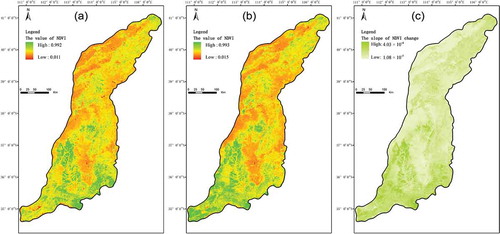
The vegetation changes in the TMR result in the blue water decrease and green water increase. Figure 9 shows the changes in the four main types of land use/land cover in the research region. Urban areas have clearly expanded and agricultural land and grassland have been converted to each other to some extent. Forest land has increased and benefited from the implementation of some policies (e.g. conversion of farmland to forests for soil and water conservation). To determine the changes in the vegetation due to this conversion, a linear regression method was used and the slope of the maximum NDVI (MODIS dataset, 500 m × 500 m) in March of 2000 and 2015 was calculated. The spatial distribution of the NDVI in 2010 and 2015 and the annual average slope from 2000 to 2015 are shown in Figure 10(a), (b) and (c), respectively. The positive gradient of the NDVI (Fig. 10(c)) and the similar spatial distributions indicate that the quantity of vegetation in the TMR has improved since 2000. This improvement results in an increase in the green water and decrease in the blue water due to greater canopy interception, higher regional roughness values, and longer concentration time. These results illustrate why the gap between the blue water and green water has further expanded since 2000, which is shown in Figure 5.

Figure 9. Land-use/land-cover statistics in five periods.

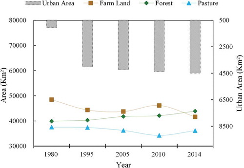
Figure 10. Distribution and slope of NDVI in the TMR in (a) March 2010 and (b) March 2015. (c) Change in slope of NDVI (year⁻¹) from 2000 to 2015.

In this study, the impacts of climate change and human activities on the changes in the blue water and green water have been qualitatively analysed, however, a quantitative analysis is the key point of subsequent research.

4.2 Comparison with previous studies

Several previous studies have provided related conclusions on the spatio-temporal changes in the runoff (i.e. blue water in this study). For instance, Liu and Zhang (2004) indicated that the contribution rate of climate change to runoff reduction in the Middle Yellow River Basin was 43%. The LUCC in the Yellow River Basin accounts for no less than 50% of the decrease in runoff (Zhang et al. 2008). Yang et al. (2015) indicated that the contribution rate of the precipitation decrease to the runoff reduction of the Yellow River was 49.3%. A study of blue water and green water in the Weihe River Basin also concluded that the blue water decreased and the green water increased (Zuo et al. 2015). Xu et al. (2014) showed that the blue water decreased in the period from 1956 to 2005.

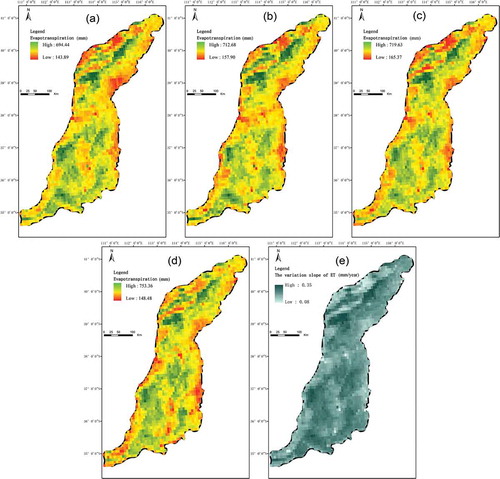
A comparison of the simulated green water and the remote sensing-based ET from the global 8 km × 8 km product (Zhang et al. 2009, 2010, 2015) was carried out in this study. The remote sensing-based ET in 1983, 1993, 2003 and 2013, and the change in the slope of the ET from 1983 to 2013 are shown in Figure 11(a), (b), (c), (d) and (e), respectively. Because the green water (i.e. a part of the actual ET) is defined as the rainwater directly used by the vegetation, the value is smaller than the remote sensing-based ET. Figure 11 indicates that the ET is bigger in the YRBP than in the HRBP and the actual ET is higher in the regions with more farmland. Moreover, there is an increasing trend of the ET in all the sub-basins in the TMR. Therefore, the results of this study agree well with those of previous studies.

Figure 11. Distribution and slope of ET in the TMR in (a) 1983, (b) 1993, (c) 2003 and (d) 2013. (e) Change in slope of ET (mm/year) from 1982 to 2013.

4.3 Disadvantages and perspectives

The performance of the distributed hydrological model WEP-L relies on the accuracy and resolution of the input data and the calibration of the model. Although important discoveries have been revealed by this research, we have to point out that there are also some limitations.

The first limitation is the uncertainty of the model. Any hydrological model inevitably has uncertainty. Even though the WEP-L model used in this study provides relative low simulation errors and has the ability to describe the water cycle processes in the TMR, there is still room for improvement in the model calibration to reduce the uncertainties. It can be seen that the model simultaneously overestimates the flood peak flow and the runoff in the dry season at the Wuzhi hydro-station, which suggests further adjustments of the parameters are still needed. For instance, a lower saturated hydraulic conductivity coefficient of the soil surface may reduce the infiltration and lead to overestimation of the flood peak. A greater thickness of the soil layers and a larger specific yield of the unconfined aquifer may increase the subsurface runoff and then overestimate the runoff in the dry season.

The challenge of the parameter optimization of PBDHMs still exists because of a series of problems that are difficult to solve, such as the numerous model parameters, the equivalence of different parameters, and the time-consuming calculations. These problems are compounded when the parameters are adjusted manually to calibrate a PBDHM. However, several scholars have already made such progress. Ajami et al. (2004) used the shuffled complex evolution–University of Arizona (SCE-UA) algorithm to calibrate the semi-distributed hydrological model SWAT. Chen et al. (2016) developed an improved method based on the particle swarm optimization (PSO) algorithm for parameter optimization of the Liuxihe model in catchment flood forecasting. These studies serve as a continually useful reference for further research on the calibration of PBDHMs. We plan to calibrate the WEP-L model more effectively based on a correlation analysis in the next study.

The second limitation is insufficient information available for mountainous areas because of the sparse monitoring stations (hydro-stations, meteorological stations), especially at high altitudes; this affects the availability and accuracy of the input meteorological and runoff data and adds uncertainties to the simulation of the hydrological processes. In addition, the relatively coarse spatio-temporal resolution of the land-use data has an impact on the simulation performance. There may be some adverse effects due to the coarse classification of the land-use/land-cover types. The land-use/land-cover data used in the model were created according to the China national standard GB/T 21010-2007, in which the first-grade classification forest land contains only woodland, shrubland and other forest land; grassland is further classified into three subclasses of natural grassland, artificial grassland and other grassland. The vegetation community structure improves after forest planting and the LAI may vary greatly in different time periods, which significantly influences the processes of runoff generation and confluence.

However, these problems could be solved by integrated applications of new technology, such as optical remote sensing technology, active and passive microwave remote sensing technology, computer technology, and data assimilation technology. We will continue to investigate relevant methods to improve the simulation of the water cycle processes.

5 Conclusion

In summary, we simulate the water cycle processes based on a PBDHM, analyse the changes in the blue and green water from 1956 to 2015, and summarize the temporal and spatial changes in the Taihang Mountain Region. The main conclusions of the study are as follows.

Over the recent 60 years (1956–2015), climate change and vegetation improvements have changed the water cycle of the TMR in the following manner: the precipitation decreases (−1.39 mm/year), the temperature rises (0.025°C/year), the blue water decreases (−0.72 mm/year) and the green water increases (1.49 mm/year). In the period 2011–2015, the annual average blue water decreased by 7.31 × 10⁹ m³, while the annual average green water increased by 13.60 × 10⁹ m³, compared to the values in the period 1956–1960.

During the course of a year, the ranking of the amount of seasonal blue water in the TMR in descending order is summer, autumn, spring and winter, while the ranking for green water is summer, spring, autumn and winter. With respect to the spatial distribution, the precipitation, blue water and green water are higher on the windward slopes than on the leeward slopes of the TMR. The blue water yield is generally higher in forest and grassland than in farmland, while the distribution of green water is the opposite.

Compared with green water, blue water is more active and the changes are more random and exhibit sensitivity to climate change (especially precipitation change). It is also demonstrated that the robust water cycle processes of green water have low volatility in the TMR. There are obvious geographical differences in the intensity changes of blue and green water between the YRBP and HRBP. The change in intensity of blue water is greater in the YRBP than in the HRBP, while the differences are relatively small for green water.

In the TMR, the current amount of green water is already 55% higher than the amount of blue water, and the fact that the quantity and quality of the vegetation have improved means that the water resources shared by ecosystems will further increase. Hence, more attention should be paid to the competition for water use in future ecological and socio-economic developments. This study provides not only the scientific basis for the coordinated development of ecosystems and socio-economic systems, but also useful information for water resources regulation and control in other similar mountainous regions.

Disclosure statement

No potential conflict of interest was reported by the authors.

Additional information

Funding

This study is funded by the following projects: the National Basic Research Program of China (973 Program) under Grant No. [2015CB452701], the National Key Research and Development Program of China under Grant No. [2016YFC0401301] and [2017YFC0405803], Ministry of Science and Technology, PRC.

References

- Abbaspour, K.C., et al., 2009. Assessing the impact of climate change on water resources in Iran. Water Resources Research, 45 (10), W10434–W10435. doi:10.1029/2008WR007615
- Ajami, N.K., et al., 2004. Calibration of a semi-distributed hydrologic model for streamflow estimation along a river system. Journal of Hydrology, 298 (1–4), 112–135. doi:10.1016/j.jhydrol.2004.03.033
- Arnold, J. and Allen, P., 1996. Estimating hydrologic budgets for three Illinois watersheds. Journal of Hydrology, 176 (1–4), 57–77. doi:10.1016/0022-1694(95)02782-3
- Chen, Y., et al., 2011. Liuxihe model and its modeling to river basin flood. Journal of Hydrologic Engineering, 16 (2), 33–50. doi:10.1061/(ASCE)HE.1943-5584.0000286
- Chen, Y., Li, J., and Xu, H., 2016. Improving flood forecasting capability of physically based distributed hydrological models by parameter optimization. Hydrology and Earth System Sciences, 20 (1), 375–392. doi:10.5194/hess-20-375-2016
- Falkenmark, M., 1997. Meeting water requirements of an expanding world population. Philosophical Transactions of the Royal Society B: Biological Sciences. 352 (1356), 929–936.
- Falkenmark, M., 1999. Forward to the Future: A Conceptual Framework for Water Dependence. Ambio, 28 (4), 356–361.
- Falkenmark, M., Rockstr, M.J., and Karlberg, L., 2009. Present and future water requirements for feeding humanity. Food Security, 1 (1), 59–69. doi:10.1007/s12571-008-0003-x
- Falkenmark, M. and Rockström, J., 2006. The new blue and green water paradigm: breaking new ground for water resources planning and management. Journal of Water Resources Planning & Management, 132 (3), 129–132. doi:10.1061/(ASCE)0733-9496(2006)132:3(129)
- Falkenmark, M. and Rockström, J., 2010. Building water resilience in the face of global change: from a blue-only to a green-blue water approach to land-water management. Journal of Water Resources Planning and Management, 136 (6), 606–610. doi:10.1061/(ASCE)WR.1943-5452.0000118
- Feng, X., et al., 2016. Revegetation in China’s Loess Plateau is approaching sustainable water resource limits. Nature Climate Change, 6 (11). 1019–1022.
- Gerten, D., et al., 2005. Contemporary “green” water flows: simulations with a dynamic global vegetation and water balance model. Physics and Chemistry of the Earth, Parts A/B/C, 30 (6–7), 334–338. doi:10.1016/j.pce.2005.06.002
- Glavan, M., Pintar, M., and Volk, M., 2013. Land use change in a 200-year period and its effect on blue and green water flow in two Slovenian Mediterranean catchments-lessons for the future. Hydrological Processes, 27 (26), 3964–3980. doi:10.1002/hyp.v27.26
- Gupta, H.V., Sorooshian, S., and Yapo, P.O., 1999. Status of automatic calibration for hydrologic models: comparison with multilevel expert calibration. Journal of Hydrologic Engineering, 4 (2), 135–143. doi:10.1061/(ASCE)1084-0699(1999)4:2(135)
- Hoff, H., et al., 2010. Greening the global water system. Journal of Hydrology, 384 (3–4), 177–186. doi:10.1016/j.jhydrol.2009.06.026
- Jia, Y., et al., 2001. Development of WEP model and its application to an urban watershed. Hydrological Processes, 15 (11), 2175–2194. doi:10.1002/(ISSN)1099-1085
- Jia, Y., et al., 2006. Development of the WEP-L distributed hydrological model and dynamic assessment of water resources in the Yellow River basin. Journal of Hydrology, 331 (3–4), 606–629. doi:10.1016/j.jhydrol.2006.06.006
- Jia, Y., et al., 2009. Distributed modeling of land surface water and energy budgets in the inland Heihe river basin of China.pdf. Hydrology and Earth System Sciences, 13, 1849–1866.
- Jia, Y., et al., 2012. Attribution of water resources evolution in the highly water-stressed Hai River Basin of China. Water Resources Research, 48, 2. doi:10.1029/2010WR009275
- Jia, Y., Kinouchi, T., and Yoshitani, J., 2005. Distributed hydrologic modeling in a partially urbanized agricultural watershed using water and energy transfer process model. Journal of Hydrologic Engineering, 10 (4), 253–263. doi:10.1061/(ASCE)1084-0699(2005)10:4(253)
- Kendall, M., 1975. Rank Correlation Measures [M]. London: Charles Griffin.
- Liang, X., et al., 1994. A simple hydrologically based model of land surface water and energy fluxes for general circulation models. Journal of Geophysical Research: Atmospheres. 99 (D7), 14415–14428.
- Liu, C. and Zhang, X., 2004. Causal analysis on actual water flow reduction in the mainstream of the Yellow River. Acta Geographica Sinica, 59 (3), 320–323. [in Chinese].
- Liu, J., et al., 2007a. GEPIC – modelling wheat yield and crop water productivity with high resolution on a global scale. Agricultural Systems, 94 (2), 478–493. doi:10.1016/j.agsy.2006.11.019
- Liu, J. and Yang, H., 2010. Spatially explicit assessment of global consumptive water uses in cropland: green and blue water. Journal of Hydrology, 384 (3–4), 187–197. doi:10.1016/j.jhydrol.2009.11.024
- Liu, J., Zehnder, A.J.B., and Yang, H., 2007b. Historical trends in China‘s virtual water trade. Water International, 32 (1), 78–90. doi:10.1080/02508060708691966
- Liu, X., et al., 2009. Quantifying the effect of land use and land cover changes on green water and blue water in northern part of China. Hydrology & Earth System Sciences, 13 (6), 735–747. doi:10.5194/hess-13-735-2009
- Ma, Z., et al., 2008. Analysis of impacts of climate variability and human activity on streamflow for a river basin in arid region of northwest China. Journal of Hydrology, 352 (3–4), 239–249. doi:10.1016/j.jhydrol.2007.12.022
- Mekonnen, M.M. and Hoekstra, A.Y., 2010. A global and high-resolution assessment of the green, blue and grey water footprint of wheat. Hydrology and Earth System Sciences, 14 (7), 1259–1276. doi:10.5194/hess-14-1259-2010
- Nash, J.E. and Sutcliffe, J.V., 1970. River flow forecasting through conceptual models part I — a discussion of principles. Journal of Hydrology, 10 (3), 282–290. doi:10.1016/0022-1694(70)90255-6
- Oki, T. and Kanae, S., 2006. Global hydrological cycles and world water resources. Science, 313 (5790), 1068–1072. doi:10.1126/science.1128845
- Pettitt, A.N., 1979. A non-parametric approach to the change-point problem. Applied Statistics, 28 (2), 126–135. doi:10.2307/2346729
- Postel, S.L., Daily, G.C., and Ehrlich, P.R., 1996. Human appropriation of renewable freshwater. Science, 271 (5250), 785–788.
- Rockström, J., 1999. On-farm green water estimates as a tool for increased food production in water scarce regions. Physics and Chemistry of the Earth, Part B: Hydrology, Oceans and Atmosphere, 24 (4), 375–383.
- Rost, S., et al., 2008. Agricultural green and blue water consumption and its influence on the global water system. Water Resources Research, 44 (9), 137–148. doi:10.1029/2007WR006331
- Schmitz, C., et al., 2013. Blue water scarcity and the economic impacts of future agricultural trade and demand. Water Resources Research, 49 (6), 3601–3617. doi:10.1002/wrcr.20188
- Schuol, J., et al., 2008. Modeling blue and green water availability in Africa. Water Resources Research, 44, 7. doi:10.1029/2007WR006609
- Siebert, S. and Döll, P., 2008. The Global Crop Water Model (GCWM): documentation and first results for irrigated crops. Frankfurt am Main: Germany: Institute of Physical Geography, University of Frankfurt.
- Siebert, S. and Döll, P., 2010. Quantifying blue and green virtual water contents in global crop production as well as potential production losses without irrigation. Journal of Hydrology, 384 (3–4), 198–217. doi:10.1016/j.jhydrol.2009.07.031
- Sun, C. and Ren, L., 2013. Assessment of surface water resources and ET in the Haihe River basin of China using SWAT model. Hydrological Processes, 27 (8), 1200–1222. doi:10.1002/hyp.9213
- Veettil, A.V. and Mishra, A.K., 2016. Water security assessment using blue and green water footprint concepts. Journal of Hydrology, 542, 589–602. doi:10.1016/j.jhydrol.2016.09.032
- Vörösmarty, C.J., et al., 2000. Global water resources: vulnerability from climate change and population growth. Science, 289 (5477), 284–288.
- Vörösmarty, C.J., et al., 2010. Global threats to human water security and river biodiversity. Nature, 467 (7315), 555–561. doi:10.1038/nature09440
- Wang, Z.M., And, B.O., and De Smedt, F., 1996. A distributed model for water and energy transfer between soil, plants and atmosphere (WetSpa). Physics and Chemistry of the Earth, 21 (3), 189–193. doi:10.1016/S0079-1946(97)85583-8
- Xia, J., et al., 2004. Water security problem and research perspective in North China. Journal of Natural Resources, 19 (5), 550–560.
- Xia, J., et al., 2005. Development of distributed time-variant gain model for nonlinear hydrological systems. Science in China Series D: Earth Sciences. 48 (6), 713.
- Xia, J., et al., 2007. Towards better water security in North China. Water Resources Management, 21 (1), 233–247. doi:10.1007/s11269-006-9051-1
- Xu, J., 2013. Effects of climate and land-use change on green-water variations in the Middle Yellow River, China. Hydrological Sciences Journal, 58 (1), 106–117. doi:10.1080/02626667.2012.746462
- Xu, X., et al., 2014. Attribution analysis based on the Budyko hypothesis for detecting the dominant cause of runoff decline in Haihe basin. Journal of Hydrology, 510 (6), 530–540. doi:10.1016/j.jhydrol.2013.12.052
- Xu, Z.X., et al., 2005. Long-term trend analysis for precipitation in Asian Pacific FRIEND river basins. Hydrological Processes, 19 (18), 3517–3532. doi:10.1002/(ISSN)1099-1085
- Xu, Z.X., Takeuchi, K., and Ishidaira, H., 2003. Monotonic trend and step changes in Japanese precipitation. Journal of Hydrology, 279 (1–4), 144–150. doi:10.1016/S0022-1694(03)00178-1
- Yang, D., Herath, S., and Musiake, K., 1998. Development of a geomorphology-based hydrological model for large catchments. Proceedings of Hydraulic Engineering, 42, 169–174. doi:10.2208/prohe.42.169
- Yang, D., Zhang, S., and Xu, X., 2015. Attribution analysis for runoff decline in Yellow River Basin during recent fifty years based on Budyko hypothesis. Sci Sin Tech, 45 (10), 1024–1034. [in Chinese].
- Yang, H. and Zehnder, A., 2007. Virtual water”: an unfolding concept in integrated water resources management. Water Resources Research, 43 (12). doi:10.1029/2007WR006048
- Zang, C., et al., 2015. Influence of human activities and climate variability on green and blue water provision in the Heihe River Basin, NW China. Journal of Water and Climate Change, jwc2015194 doi:10.2166/wcc.2015.194.
- Zhang, K., et al., 2009. Satellite based analysis of northern ET trends and associated changes in the regional water balance from 1983 to 2005. Journal of Hydrology, 379 (1), 92–110. doi:10.1016/j.jhydrol.2009.09.047
- Zhang, K., et al., 2010. A continuous satellite-derived global record of land surface ET from 1983 to 2006. Water Resources Research, 46 (9), 109–118. doi:10.1029/2009WR008800
- Zhang, K., et al., 2015. Vegetation greening and climate change promote multidecadal rises of global land ET. Scientific Reports, 5 (2), 75–77.
- Zhang, W., et al., 2014. Spatiotemporal change of blue water and green water resources in the headwater of Yellow River Basin, China. Water Resources Management, 28 (13), 4715–4732. doi:10.1007/s11269-014-0769-x
- Zhang, X., et al., 2008. Responses of streamflow to changes in climate and land use/cover in the Loess Plateau, China. Water Resources Research, 44, 7. doi:10.1029/2007WR006711
- Zhuo, L., et al., 2016. Inter- and intra-annual variation of water footprint of crops and blue water scarcity in the Yellow River basin (1961–2009). Advances in Water Resources, 87, 29–41. doi:10.1016/j.advwatres.2015.11.002
- Zuo, D., et al., 2012. Spatiotemporal variations and abrupt changes of potential ET and its sensitivity to key meteorological variables in the Wei River basin, China. Hydrological Processes, 26 (8), 1149–1160. doi:10.1002/hyp.8206
- Zuo, D., et al., 2015. Simulating spatiotemporal variability of blue and green water resources availability with uncertainty analysis. Hydrological Processes, 29 (8), 1942–1955. doi:10.1002/hyp.v29.8