Regional assimilation of in situ observed soil moisture into the VIC model considering spatial variability

ABSTRACT

In order to improve the soil moisture (SM) modelling capacity, a regional SM assimilation scheme based on an empirical approach considering spatial variability was constructed to assimilate in situ observed SM data into a hydrological model. The daily variable infiltration capacity (VIC) model was built to simulate SM in the Upper Huai River Basin, China, with a resolution of 5 km × 5 km. Through synthetic assimilation experiments and validations, the assimilated SM was evaluated, and the assimilation feedback on evapotranspiration (ET) and streamflow are analysed and discussed. The results show that the assimilation scheme improved the SM modelling capacity, both spatially and temporally. Moreover, the simulated ET was continually affected by changes in SM simulation, and the streamflow predictions were improved after applying the SM assimilation scheme. This study demonstrates the potential value of in situ observations in SM assimilation, and provides valuable ways for improving hydrological simulations.

KEYWORDS:

• soil moisture
• regional assimilation
• VIC model
• spatial variability

Editor A. Castellarin Guest editor Y. Chen

1 Introduction

Soil moisture (SM) is a key state variable in numerous environmental disciplines; it controls a variety of land surface fluxes and energy processes, and plays a vital role in hydrological processes such as runoff, infiltration and evapotranspiration (ET) (Seneviratne et al. 2010). Therefore, obtaining accurate SM information is a priority for many hydro-meteorological applications, including drought monitoring, water management and rainfall-runoff prediction (Sahoo et al. 2013, Enenkel et al. 2016).

Ground measurements and satellite remote sensing are the two main sources of SM observations. Ground-based techniques are the only way to obtain accurate multi-layer SM observations at the point scale. However, the sparse and discontinuous point observations obtained by these methods cannot represent regional SM values well since the SM values are highly variable in both space and time (Crow et al. 2012). Compared to in situ observations, satellite retrieval can provide continuous SM data on a large scale. In particular, microwave remote sensing observations can be collected without time or weather restrictions, which has great potential in SM monitoring. However, satellite observations can only provide SM information for the surface soil layer (Gao et al. 2006, Brocca et al. 2010, Escorihuela et al. 2010). Besides, satellite retrieval is closely affected by soil type, surface roughness and vegetation coverage, which may cause some observational uncertainties and lead to a lack of spatial and temporal coverage (Gruhier et al. 2010, Shi et al. 2011).

Hydrological models based on long-term meteorological observations are alternative and valid solutions for obtaining SM data (Wu et al. 2007). Long series and spatially continuous SM data can be expected over large scales with the application of hydrological models (Boone et al. 2004, Du et al. 2016). Hydrological models can adequately reflect the dynamic changes and spatial patterns of SM values. In particular, distributed hydrological models divide the whole catchment into a number of grid cells at fine resolution, for example, the variable infiltration capacity (VIC) model (Liang et al. 1994, 1996), the WEP-L model (Jia et al. 2001) and the Liuxihe model (Chen et al. 2011b). Among these models, the VIC model is widely used in SM simulation, since it uses a spatial probability distribution function to represent sub-grid variability in the SM storage capacity, which can give a more realistic treatment of the simulated SM within a model grid cell (Wu et al. 2007, 2011). However, the modelled SM values contain uncertainties which are mainly caused by the model structure, meteorological forcings and parameter errors (Tramblay et al. 2011, Mo and Lettenmaier 2014, Massari et al. 2015). Consequently, it is necessary to effectively and efficiently assimilate observational data into hydrological models using data assimilation methods, which can reduce uncertainties in the SM simulations (Reichle et al. 2002, Draper et al. 2011, Dumedah and Coulibaly 2013).

Over the past few decades, sequential data assimilation methods, such as the extended or ensemble Kalman filter (Draper et al. 2012, de Rosnay et al. 2013, Kolassa et al. 2017), have been widely used in SM assimilation. These methods provide techniques for quantifying errors in both observations model predictions, with the aim to optimally merge data provided from uncertain observations and uncertain model predictions (Reichle and Koster 2004, Alvarez-Garreton et al. 2015). Even though model simulations are improved to some extent with the application of SM assimilation, assimilation scheme still presents a number of controversial issues, in particular, for bias corrections and error quantification (Liu et al. 2012, Alvarez-Garreton et al. 2015, Massari et al. 2015).

Affected by uncertainties in the SM simulations, the model-based SM product is biased compared to the observations (Brocca et al. 2011, Sahoo et al. 2013). However, bias is not desired in sequential data assimilation methods and bias correction is often used to address bias between model simulations and observations. Most of the bias correction methods used in SM assimilation rescale the observations to the model simulations, and only validate the assimilation results in terms of temporal change instead of absolute magnitudes (e.g. Kumar et al. 2012, Lievens et al. 2015). This means that the assimilated SM series is still biased compared to the original observations, which is unfavorable to the acquisition of an accurate SM product. Therefore, in this study, the assimilated SM relatively will be corrected to the observational patterns after assimilation, and reliable in situ observed SM data will be selected and assimilated into the hydrological model instead of the biased and uncertain satellite observations. Nevertheless, previous assimilation schemes using in situ observations are often employed at the point or local scale (e.g. Walker et al. 2001, De Lannoy et al. 2007, Fairbairn et al. 2015), which does not support the regional SM assimilation.

The accurate quantification of the simulation and observation errors is another key point for the SM assimilation. To achieve an optimal estimation, data assimilation algorithms require prior knowledge of the product uncertainties. For example, the commonly used ensemble Kalman filter (Evensen 1994, 2003) updates the model error information through generating a prediction ensemble by perturbing the model parameters or meteorological forcings (Dumedah and Coulibaly 2013, Sahoo et al. 2013), and the observational error is often treated as an independent Gaussian noise with fixed variance (Han et al. 2012, Massari et al. 2015). As a result, the relative weights between the model simulations and the observations are theoretically subjective (Yilmaz et al. 2012), which may affect the optimality of the SM assimilation. Even though the existing triple collocation (TC) method could estimate the random error objectively (Crow and van den Berg 2010, Dorigo et al. 2010, Yilmaz et al. 2012), the error estimates of each product are constant in time and the corrective information is not temporally propagated forward.

Regional assimilation based on in situ observed SM data is mainly restricted by the scale mismatch between in situ observations and model simulations since the SM values are highly variable. However, the SM spatial variability is also variable, both in space and in time. This means that the representativeness of the in situ observed SM values is spatially and temporally different. The stronger SM variability causes the weaker representativeness of the in situ observations and vice versa. Therefore, a more objective and efficient assimilation scheme can be realized if assimilating in situ observed SM into a hydrological model considering spatial variability.

In this study, a regional SM assimilation scheme based on an empirical approach that considers spatial variability is constructed to assimilate in situ observed SM into a hydrological model. In the empirical approach, the relative weights between the model and observations are efficiently determined according to the spatial variability. To conduct the assimilation scheme, a daily VIC model with a spatial resolution of 5 km × 5 km is constructed. With the application of the assimilation scheme, the in situ observed SM values are assimilated into the VIC model with a view to improving the SM simulations. Furthermore, the assimilation feedback for the ET and streamflow data are also analysed in order to fully understand the assimilation scheme.

2 Data and methodology

2.1 Study site and data sources

The Upper Huai River Basin (UHRB, Zou et al. 2017), up to Wangjiaba station, draining 30 630 km², was selected as the study area (Fig. 1). The UHRB plays a critical role in flood control and water management the entire Huai River Basin (HRB), which is an important agricultural area in eastern China.

Figure 1. Station distribution in the study area, the Upper Huai River Basin, China.

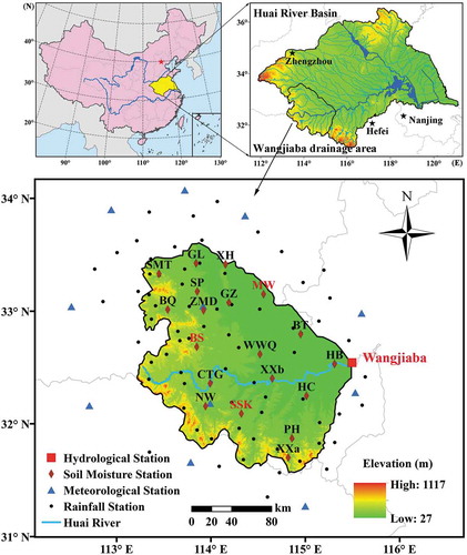
Soil moisture data from January 2012 to December 2014 derived from 19 stations in the UHRB (Fig. 1) were provided by the Chinese Ministry of Water Resources Information Center (CMWRIC). The gravimetric SM data in a soil layer of 0–10 cm were measured artificially using the oven-drying method, with an observational frequency of three times per month (1st, 11th and 21st at 08:00 h). In order to be consistent with the model-based SM values, the gravimetric SM values were converted to volumetric SM using soil bulk density data from the Food and Agriculture Organization of the United Nations (FAO; http://www.fao.org/soils-portal/). Additionally, to make it easier to understand the effects of the assimilation scheme, three typical stations, Shishankou (SSK), Miaowan (MW) and Boshan (BS), were selected for the time series analysis.

To drive the VIC model, meteorological forcing data of air temperature (maximum, minimum, and mean) and precipitation from January 1989 to December 2014 were used in this study (Fig. 1). The forcing data were collected from 11 national meteorological stations and 44 rainfall stations located in and around the UHRB, and were provided by three organizations: the National Meteorological Information Centre of the China Meteorological Administration (http://data.cma.cn/), CMWRIC, and the Hydrology Bureau of the Huai River Conservancy Commission. In addition, daily streamflow records at Wangjiaba station from January 1989 to December 2014 were provided by the CMWRIC and used for model calibration and verification.

2.2 VIC model

The VIC macroscale semi-distributed hydrological model was adopted in this study to simulate SM data. The daily VIC model was constructed in the UHRB with a spatial resolution of 5 km × 5 km (1265 grids in total). The VIC model was driven by observed daily maximum and minimum air temperature and precipitation, which were estimated on 5 km × 5 km grids derived from 11 long-term meteorological stations and 44 rainfall stations in and around the UHRB (Fig. 1) using the inverse distance weighting (IDW) method. The influence of topography on precipitation was not considered in the IDW method; however, the relationship between temperature and elevation was considered such that each 100-m elevation increment resulted in a 0.65°C temperature increase.

The parameters used for the VIC model can be divided into four categories: geography, vegetation, soil, and hydrological. The geographical parameters were calculated based on the meteorological variables and the location of the UHRB. For each grid point, the global 10-km soil profile dataset (Reynolds et al. 2000) and the global 1-km land cover classification dataset released by the University of Maryland, USA (Hansen et al. 2000) were used to define the model soil and vegetation parameters. The hydrological parameters are difficult to determine directly due to the uncertainties in the model and complex runoff processes (Chen et al. 2016). Accordingly, the models usually need to be calibrated, and hydrological parameters were calibrated using the observed streamflow data at Wangjiaba station in this study. An auto-optimization procedure (Rosenbrock 1960) was used for model calibration. More details of the model building and parameters determination can be found in Wu et al. (2007, 2011) and Mao et al. (2017).

The VIC model can simulate daily volumetric SM values in three soil layers. The first SM layer was fixed at 10 cm, while the depth of the second and third layers was determined through the model calibration process. In order to keep consistency with the in situ observations, only the SM values in the first model layer (0–10 cm) were used in the SM assimilation, and the assimilation period was set as January 2012 to September 2014.

2.3 Data assimilation scheme

The data assimilation scheme is divided into six parts, the overall framework is shown in Fig. 2. The rescaling (Section 2.3.1) and bias correction (Section 2.3.6) are used as a priori and a posteriori processing techniques for the observed and assimilation updated SM values (hereafter referred to as updated SM), respectively. The spatial variability (sections 2.3.3 and 2.3.4) and regional assimilation (Section 2.3.5) are two main factors considered in this scheme. The methods in sections 2.3.1 to 2.3.3 are only conducted for the observed VIC grids, while those in sections 2.3.4 to 2.3.6 are conducted for all VIC grids.

Figure 2. Flowchart of the data assimilation scheme.

Figure 3. Ensemble members of simulated and observed SM values.

2.3.1 Rescaling of in situ observations

As mentioned in Section 1, a systematic difference exists between observed and simulated SM values due to the spatial mismatch and model uncertainties (Reichle and Koster 2004, Chen et al. 2011a). Direct assimilation of systematically different observations into hydrological models may result in inconsistency between the state and model SM parameters, and an increase in model uncertainty. Therefore, a significant prerequisite for data assimilation is the presence of zero mean, temporally uncorrelated forecast and observational errors (Sahoo et al. 2013). The most commonly used bias processing method is to rescale the observations to the simulations before SM assimilation (e.g. Kumar et al. 2012, Lievens et al. 2015).

After practicing several rescaling methods, including the first-order moment (long-term mean) rescaling, the first and second-order moments (mean and standard deviation) rescaling and the cumulative distribution function (cdf) rescaling (Liu et al. 2011), the first-order moment rescaling of the long-term mean recommended by Lievens et al. (2015), was selected as the best a priori processing technique to use for SM observations in the data assimilation system, as follows:

(1) ${\mathrm{S}\mathrm{M}}_i^{\mathrm{o}\mathrm{b}\mathrm{s}\ast }=\overline{{\mathrm{S}\mathrm{M}}_i^{\mathrm{s}\mathrm{i}\mathrm{m}}}{+(\mathrm{S}\mathrm{M}}_i^{\mathrm{o}\mathrm{b}\mathrm{s}}-\overline{{\mathrm{S}\mathrm{M}}_i^{\mathrm{o}\mathrm{b}\mathrm{s}}})$(1)

with $\overline{{\mathrm{S}\mathrm{M}}_i^{\mathrm{s}\mathrm{i}\mathrm{m}}}$ denoting the 3-year (2012–2014) mean of the SM simulations, ${\mathrm{S}\mathrm{M}}_i^{\mathrm{o}\mathrm{b}\mathrm{s}\ast }$ is the rescaled in situ SM observation, and $\overline{{\mathrm{S}\mathrm{M}}_i^{\mathrm{o}\mathrm{b}\mathrm{s}}}$ is the 3-year mean of the SM observations, which were located in the corresponding VIC grid i. The first-order rescaling is easy to practice, and can best preserve the dynamic change of the observational time series.

2.3.2 Data assimilation algorithm

In this study, an empirical approach with the consideration of spatial variability is proposed and employed to sequentially assimilate in situ observed SM into the VIC model. The empirical approach is a computationally inexpensive approach based on the EnKF idea. State variable forecast and update are the two main components involved in the empirical approach. In the forecast part, the state variable, set as the simulated SM value, is predicted by the VIC model at time step t in grid i using:

(2) ${\mathrm{S}\mathrm{M}}_{i,t}^{\mathrm{s}\mathrm{i}\mathrm{m}}=\mathrm{V}\mathrm{I}\mathrm{C}\left({\mathrm{S}\mathrm{M}}_{i,t-1}^{\mathrm{u}\mathrm{p}\mathrm{d}}\right)$(2)

where $\mathrm{V}\mathrm{I}\mathrm{C}\left(\cdot \right)$ is the VIC model operator, ${\mathrm{S}\mathrm{M}}_{i,t}^{\mathrm{s}\mathrm{i}\mathrm{m}}$ and ${\mathrm{S}\mathrm{M}}_{i,t-1}^{\mathrm{u}\mathrm{p}\mathrm{d}}$ are the simulated SM values at time step t and the updated SM value at the last time step t–1, respectively.

In the update part, the simulated SM is updated using the scaled observational SM ${\mathrm{S}\mathrm{M}}_{i,t}^{\mathrm{o}\mathrm{b}\mathrm{s}\ast }$ according to:

(3) ${\mathrm{S}\mathrm{M}}_{i,t}^{\mathrm{u}\mathrm{p}\mathrm{d}}={\mathrm{S}\mathrm{M}}_{i,t}^{\mathrm{s}\mathrm{i}\mathrm{m}}+K_{i,t}({\mathrm{S}\mathrm{M}}_{i,t}^{\mathrm{o}\mathrm{b}\mathrm{s}\ast }-H{\mathrm{S}\mathrm{M}}_{i,t}^{\mathrm{s}\mathrm{i}\mathrm{m}})$(3)

where ${\mathrm{S}\mathrm{M}}_{i,t}^{\mathrm{u}\mathrm{p}\mathrm{d}}$ is the updated SM value at time step t, H is the observation operator, being 1 in this scheme as the prediction and observation both are SM in the study; K_i,t is the weighting factor, which was determined by the simulation error variance $P_{i,t}^f$ and the observation error variance R_i,t:

(4) $K_{i,t}=P_{i,t}^f{H}^T{\left[H{P}_{i,t}^f{H}^T+R_{i,t}\right]}^{-1}$(4)

The calculation processes of $P_{i,t}^f$ and R_i,t are described in Section 2.3.3.

2.3.3 Spatial variability consideration

As mentioned in Section 1, ensembles of model predictions and observations in the EnKF are often generated by randomly perturbing model forcings and observations. As a result, the assimilation is restricted by the subjective weight and the time-consuming calculations. In this empirical approach, the ensembles used for the error variance ($P_{i,t}^f$ and R_i,t) calculation are generated in a different way, which contains the critical information of the spatial variability.

The observation ensembles are set as the SM observations obtained at in situ stations located within a S₀ ensemble radius circle centred around a particular grid cell, and the simulation ensembles are set as the grid-scale simulations corresponding to each of the observation members (Fig. 3). Then, the simulation and observation error variance are calculated as:

(5) $R_{i,t}=\frac{1}{N-1}\sum _{k=1}^N\left[{\mathrm{S}\mathrm{M}}_{k,t}^{\mathrm{o}\mathrm{b}\mathrm{s}\ast }-\overline{{\mathrm{S}\mathrm{M}}_t^{\mathrm{o}\mathrm{b}\mathrm{s}\ast }}\right]{\left[{\mathrm{S}\mathrm{M}}_{k,t}^{\mathrm{o}\mathrm{b}\mathrm{s}\ast }-\overline{{\mathrm{S}\mathrm{M}}_t^{\mathrm{o}\mathrm{b}\mathrm{s}\ast }}\right]}^T$(5)

(6) $P_{i,t}^f=\frac{1}{N-1}\sum _{k=1}^N\left[{\mathrm{S}\mathrm{M}}_{k,t}^{\mathrm{s}\mathrm{i}\mathrm{m}}-\overline{{\mathrm{S}\mathrm{M}}_t^{\mathrm{o}\mathrm{b}\mathrm{s}\ast }}\right]{\left[{\mathrm{S}\mathrm{M}}_{k,t}^{sim}-\overline{{\mathrm{S}\mathrm{M}}_t^{\mathrm{o}\mathrm{b}\mathrm{s}\ast }}\right]}^T$(6)

where N is the ensemble number, set as 3 to 5 depending on a radius S₀ of less than 75 km, k represents the kth member in the ensembles, $\overline{{\mathrm{S}\mathrm{M}}_t^{\mathrm{o}\mathrm{b}\mathrm{s}\ast }}$ is the mean value of the rescaled observed SM ensemble.

Even though the empirical assimilation approach is based on the EnKF idea, the error variances here are totally different from those in the EnKF. The simulation and observation ensembles in the empirical approach are generated directly using surrounding values instead of the ensemble prediction in the EnKF, hence the assimilation efficiency is greatly improved. In Equation (5), $\overline{{\mathrm{S}\mathrm{M}}_t^{\mathrm{o}\mathrm{b}\mathrm{s}}}$ represents the local mean SM values neighboring the assimilation grid, therefore, R_i,t represents differences between the in situ observations and the local mean SM value, which is determined by the spatial variability of the SM. For the VIC simulations, the rescaled $\overline{{\mathrm{S}\mathrm{M}}_t^{\mathrm{o}\mathrm{b}\mathrm{s}\ast }}$ in Equation (8) is used as the relative local true value since few stations could provide reliable spatial average information (Aubert et al. 2003, Brocca et al. 2010). Accordingly, the $P_{i,t}^f$ is considered as the spatial simulation error.

It is noted that the difference between the in situ observed SM value and the grid true value is mainly due to the SM spatial variability rather than the random measurement error. Therefore, the spatial variability (R_i.t) and the simulation error ($P_{i,t}^f$) are the main considerations for the updated SM value in the assimilation algorithm. The stronger of the SM spatial variability presenting over the surrounding area, the weaker the representativeness for the in situ observation representing the local SM value. The increase in spatial variability finally result in a decrease in the weighting factor in the assimilation algorithm, and then the updated SM value will be close to the VIC simulation. Similarly, with the increase in simulation error, the weighting factor increases, and the updated SM value will be close to the in situ observation.

2.3.4 Weighting factor conversion

In Section 2.3.3, the ensemble radius S₀ is bigger than the VIC grid size. As a result, the weighting factor between the local area and the assimilation grid in different.

Therefore, the spatial variation of the weighting factor was analysed for its spatial conversion at different scales. By subtracting the differences between the regional averaged SM derived from all in situ stations and randomly different number of stations, the representative effects of the in situ observations are removed. Then, the time-averaged weighting factors at different ensemble radiuses during the study period are calculated and shown in Fig. 4. The weighting factors decrease gradually and tend to be stable with the increase in radius. This demonstrate that the spatial representativeness of the in situ observed SM values decreases when the spatial scale increase, and the weighting factor guides the updated SM values close to the simulation values. However, the weighting factors vary little with the ensemble radius and are stabilized at approximately 0.5 when the radius reaches 100 km. This is reasonable and understandable, since over large scales (more than 100 km²), the representativeness of the point measurements and grid simulations is quite similar.

Limited by the sparse observation stations, the weighting factors within a smaller ensemble radius (less than 30 km) could not be obtained directly. Theoretically, a smaller ensemble radius indicates stronger representativeness of the in situ observation, with a higher weighting factor and the spatial scale becomes a point scale when the radius is 0. Accordingly, weighting factors at different ensemble radiuses are fitted with a negative exponential function (Fig. 4) and a spatial conversion coefficient, a(h) is employed to convert the weighting factors to 5-km assimilation grid at different scales. Then, Equation (3) can be replaced with:

(7) ${\mathrm{S}\mathrm{M}}_{i,t}^{\mathrm{u}\mathrm{p}\mathrm{d}}={\mathrm{S}\mathrm{M}}_{i,t}^{\mathrm{s}\mathrm{i}\mathrm{m}}+a(h)\cdot K_{i,t}(h)\cdot ({\mathrm{S}\mathrm{M}}_{i,t}^{\mathrm{o}\mathrm{b}\mathrm{s}\ast }-H{\mathrm{S}\mathrm{M}}_{i,t}^{\mathrm{s}\mathrm{i}\mathrm{m}})$(7)

2.3.5 Assimilation gain interpolation

The empirical assimilation approach was only applied for the observed VIC grid. In order to realize the lateral propagation of the assimilation effects, the assimilation gain interpolation method is applied for the non-observed VIC grid to update the simulated SM values. The assimilation gain G_i,t at the observed VIC grid is defined as:

(8) $G_{i,t}={\mathrm{S}\mathrm{M}}_{i,t}^{\mathrm{u}\mathrm{p}\mathrm{d}}-{\mathrm{S}\mathrm{M}}_{i,t}^{\mathrm{s}\mathrm{i}\mathrm{m}}$(8)

Similarly, we analysed the spatial variation of the assimilation gains and found their spatial difference (ΔG) generally increased with distance (Fig. 5). The variation can be fitted with a Gaussian function G(h), and G(h) was normalized as the weight function w(h) for the assimilation gain interpolation. Then the weight of G_i,t in the interpolation is estimated through an empirical error weight function:

(9) $w_i=exp(-4h_i^2/D_0^2)$(9)

where D₀ is the search radius, set the same as A₀ (Fig. 3) and h_i is the distance between the interpolating grid and ith grid within D₀. The assimilation gain of the non-observed VIC grid G_i,t is estimated as:

(10) $G_{j,t}=\frac{\sum _{i=1}^N(w_i{G}_{i,t})}{\sum _{i=1}^N(w_i)}$(10)

The corresponding updated SM values is then calculated as:

(11) ${\mathrm{S}\mathrm{M}}_{j,t}^{\mathrm{u}\mathrm{p}\mathrm{d}}={\mathrm{S}\mathrm{M}}_{j,t}^{\mathrm{s}\mathrm{i}\mathrm{m}}+G_{j,t}$(11)

2.3.6 Bias correction of updated SM simulations

It is noted that previous studies (e.g. Drusch et al. 2005, Kumar et al. 2012, Dorigo et al. 2015) evaluated the updated or assimilated SM values in terms of temporal change instead of absolute magnitude. As a result, the assimilated SM obtained in previous studies is still biased owing to the significant uncertainties in the simulation processes. Even though there are some uncertainties in the in situ observations, we found the two moments are quite stable in space, which can be well estimated using the kriging technique (Wu et al. 2018). Therefore, it is possible to correct the updated SM to the final assimilated SM using the first-and second-order moments rescaling method (for both the correction of long-term mean and the variable range) based on in situ observations.

For the observed VIC grid (with station inside), the two moments are directly derived from the corresponding in situ series. For the non-observed VIC grid (no station inside), the ordinary kriging (OK) technique is carried out to obtain the two bias correction parameters. The theoretical basis and feasibility of this kriging-based application is given in our previous study (Wu et al. 2018). The variogram (represented as semi-variance) is the basis of the kriging technique, which is defined as (Lakhankar et al. 2010):

(12) $\gamma (h)=\frac{1}{2N(h)}\sum _{i=1}^{N(h)}{\left[z(x_i)-z(x_{i+h})\right]}^2$(12)

where $\gamma (h)$ is the semi-variance for the interval distance class h, N(h) is the total number of sample couples for the separation interval h, and z(x_i) and z(x_i+h) are the parameters at spatial locations i and i + h, respectively. The semi-variance members can be fitted with variogram models using the least squares best-fit method. The parameters of the variogram models consist of nugget (C₀), sill (C+ C₀) and de-correlation length (A₀) (Lakhankar et al. 2010).

The variogram was employed to describe the spatial variation of the two correction parameters. Figure 6 shows the variograms of the in situ mean value and standard deviation, which were generated for study period in the UHRB. The two variograms increase with increasing distance between stations, and are best fitted to the exponential model and the linear model, respectively. Based on the variograms, the OK technique was used to obtain the spatial patterns of the two correction parameters. In addition, the Yamamoto method was used to solve the smoothing effect of the OK estimates, as detailed in Yamamoto (2005) and Yang et al. (2010).

After that, the two kriged (interpolated through OK technique) correction parameters are used to correct the updated SM, ${\mathrm{S}\mathrm{M}}_i^{\mathrm{u}\mathrm{p}\mathrm{d}}$, according to Dumedah and Walker (2014):

(13) ${\mathrm{S}\mathrm{M}}_i^{\mathrm{a}\mathrm{s}\mathrm{s}}=m_i^{\mathrm{k}\mathrm{r}\mathrm{i}}+\left({\mathrm{S}\mathrm{M}}_i^{\mathrm{u}\mathrm{p}\mathrm{d}}-\overline{{\mathrm{S}\mathrm{M}}_i^{\mathrm{u}\mathrm{p}\mathrm{d}}}\right)\frac{{\sigma }_i^{\mathrm{k}\mathrm{r}\mathrm{i}}}{{\sigma }_i^{\mathrm{u}\mathrm{p}\mathrm{d}}}$(13)

where ${\mathrm{S}\mathrm{M}}_i^{\mathrm{a}\mathrm{s}\mathrm{s}}$ is the bias-corrected SM set as the assimilated SM, $m_i^{\mathrm{k}\mathrm{r}\mathrm{i}}$ and ${\sigma }_i^{\mathrm{k}\mathrm{r}\mathrm{i}}$ are the kriged correction parameters, and $\overline{{\mathrm{S}\mathrm{M}}_i^{\mathrm{u}\mathrm{p}\mathrm{d}}}$and ${\sigma }_i^{\mathrm{u}\mathrm{p}\mathrm{d}}$ are the 3-year mean value, and standard deviation of the updated SM, respectively. The two moments rescaling is used for the correction of both bias and variable range, which is much easier to implement compared to the cdf rescaling method.

2.4 Performance metrics

The model calibration and validation are evaluated using the relative error (E_r) and the Nash-Sutcliffe model efficiency coefficient (E_c) (Nash and Sutcliffe 1970, Wu et al. 2007) as follows:

(14) $E_r=\frac{\left(\overline{Q^{\mathrm{s}\mathrm{i}\mathrm{m}}}-\overline{Q^{\mathrm{o}\mathrm{b}\mathrm{s}}}\right)}{\overline{Q^{\mathrm{o}\mathrm{b}\mathrm{s}}}}$(14)

(15) $E_c=1-\frac{\sum _{t=1}^T{\left(Q_t^{\mathrm{s}\mathrm{i}\mathrm{m}}-Q_t^{\mathrm{o}\mathrm{b}\mathrm{s}}\right)}^2}{\sum _{t=1}^T{\left(Q_t^{\mathrm{o}\mathrm{b}\mathrm{s}}-\overline{Q^{\mathrm{o}\mathrm{b}\mathrm{s}}}\right)}^2}$(15)

where $\overline{Q^{\mathrm{s}\mathrm{i}\mathrm{m}}}$ and $\overline{Q^{\mathrm{o}\mathrm{b}\mathrm{s}}}$ are the time-averaged simulated and observed discharges during the period of T, respectively. $Q_t^{\mathrm{s}\mathrm{i}\mathrm{m}}$ and $Q_t^{\mathrm{o}\mathrm{b}\mathrm{s}}$ are the simulated and observed discharges at time step t, respectively. The E_c standardizes the agreement between the simulated and observed discharges; a value closer to 1 means that the simulated discharges series agree more with the observed discharge series.

The assimilated SM and the assimilation scheme are assessed based on several metrics: the correlation coefficient (r), the coefficient of determination (R²), the bias (cm³/cm³), the unbiased root mean square error (ubRMSE, cm³/cm³), the mean relative error (MRE) and the mean absolute relative error (MARE) (Fang et al. 2011, Dumedah and Walker 2014, Sun et al. 2017):

(16) $\mathrm{B}\mathrm{i}\mathrm{a}\mathrm{s}=\frac{1}{T}\sum _{t=1}^T\left({\mathrm{S}\mathrm{M}}_t^{\mathrm{a}\mathrm{s}\mathrm{s}}-{\mathrm{S}\mathrm{M}}_t^{\mathrm{o}\mathrm{b}\mathrm{s}}\right)$(16)

(17) $\mathrm{u}\mathrm{b}\mathrm{R}\mathrm{M}\mathrm{S}\mathrm{E}=\sqrt{\frac{1}{T}\sum _{t=1}^T{\left({\mathrm{S}\mathrm{M}}_t^{\mathrm{a}\mathrm{s}\mathrm{s}}-{\mathrm{S}\mathrm{M}}_t^{\mathrm{o}\mathrm{b}\mathrm{s}}-\mathrm{B}\mathrm{i}\mathrm{a}\mathrm{s}\right)}^2}$(17)

(18) $\mathrm{M}\mathrm{R}\mathrm{E}=\frac{1}{T}\sum _{t=1}^T\frac{\left({\mathrm{S}\mathrm{M}}_t^{\mathrm{a}\mathrm{s}\mathrm{s}}-{\mathrm{S}\mathrm{M}}_t^{\mathrm{o}\mathrm{b}\mathrm{s}}\right)}{{\mathrm{S}\mathrm{M}}_t^{obs}}$(18)

(19) $\mathrm{M}\mathrm{A}\mathrm{R}\mathrm{E}=\frac{1}{M}\sum _{i=1}^M\frac{\left|{\mathrm{S}\mathrm{M}}_i^{\mathrm{a}\mathrm{s}\mathrm{s}}-{\mathrm{S}\mathrm{M}}_i^{\mathrm{o}\mathrm{b}\mathrm{s}}\right|}{{\mathrm{S}\mathrm{M}}_i^{\mathrm{o}\mathrm{b}\mathrm{s}}}$(19)

where M is the number of observational SM values in the study area, ${\mathrm{S}\mathrm{M}}_t^{\mathrm{a}\mathrm{s}\mathrm{s}}$and $S{M}_t^{\mathrm{o}\mathrm{b}\mathrm{s}}$ are the assimilated and observed SM values at time step t, respectively. ${\mathrm{S}\mathrm{M}}_i^{\mathrm{a}\mathrm{s}\mathrm{s}}$ and ${\mathrm{S}\mathrm{M}}_i^{\mathrm{o}\mathrm{b}\mathrm{s}}$ are the SM values at grid i, respectively. The ubRMSE removes the bias from the RMSE and is therefore more meaningful for describing the random errors in the SM series.

The assimilation effects on the ET are evaluated based on the relative difference (RD, %) and the cumulative relative difference (CRD, %), which are defined as:

(20) $\mathrm{R}\mathrm{D}=\frac{{\mathrm{E}\mathrm{T}}_t^{\mathrm{a}\mathrm{s}\mathrm{s}}-{\mathrm{E}\mathrm{T}}_t^{\mathrm{s}\mathrm{i}\mathrm{m}}}{{\mathrm{E}\mathrm{T}}_t^{\mathrm{s}\mathrm{i}\mathrm{m}}}\times 100\mathrm{\%}$(20)

(21) $\mathrm{C}\mathrm{R}\mathrm{D}=\frac{\sum _{t=1}^T\left({\mathrm{E}\mathrm{T}}_t^{\mathrm{a}\mathrm{s}\mathrm{s}}-{\mathrm{E}\mathrm{T}}_t^{\mathrm{s}\mathrm{i}\mathrm{m}}\right)}{\overline{\mathrm{E}{\mathrm{T}}^{\mathrm{s}\mathrm{i}\mathrm{m}}}}\times 100\mathrm{\%}$(21)

where ${\mathrm{E}\mathrm{T}}_t^{\mathrm{a}\mathrm{s}\mathrm{s}}$ and ${\mathrm{E}\mathrm{T}}_t^{\mathrm{s}\mathrm{i}\mathrm{m}}$ are the simulated ET at time step t after and before the SM assimilation, respectively. $\overline{\mathrm{E}{\mathrm{T}}^{\mathrm{s}\mathrm{i}\mathrm{m}}}$ is the averaged simulated ET during the analysis period T. The two metrics were used to reflect the dynamic change of the ET with the timely and cumulative change of the SM values.

3 Results

3.1 Model calibration and validation

The VIC model was implemented for the UHRB to perform simulations of runoff and SM on a daily time step. The VIC model was firstly calibrated based on the observed discharges at Wangjiaba station for the calibration period (1 January 1989–31 December 2003). Then, the VIC model was validated using data from Wangjiaba station for the validation period (1 January 2004–2 April 2008).

Figure 7 compares the simulated streamflow with the observed streamflow for the calibration and validation periods. The simulations are similar to the observations in both dynamic change and overall values. For the calibration and validation periods, the E_c was 0.75 and 0.85, respectively, and the E_r was 0.038, and –0.052, respectively. The VIC SM simulations are evaluated along with the assimilated SM in Section 3.2. On the whole, the performance of model constructed in this study was found to be reasonable.

3.2 Soil moisture evaluation

A complete investigation of the assimilated SM would require accurate SM reference data. However, such reference data are not available for the UHRB and such investigation beyond the scope of our study at present. Even though there are some errors retained in the in situ observations, it is the most accurate dataset with enough accuracy for the SM evaluation. On this basis, the cross-validation method (e.g. Gao et al. 2014, Wu et al. 2018) was adopted to make an objective assessment of the SM assimilation scheme since the in situ observations are independent in the cross-validation method. Besides, the assimilated SM and original VIC simulations were also compared with the in situ observations which were integrated into the assimilation process to illustrate how the assimilation scheme works, and to assess the consistency before and after assimilation, both in time series and in spatial patterns.

3.2.1 Evaluation at the typical stations

The assimilated SM time series were assessed at three typical stations, SSK, MW and BS (Fig. 1) using the correlation coefficient (r), Bias, ubRMSE and MRE, as shown in Table 1. The temporal trends of VIC simulations were generally consistent with the observational series, with a mean correlation coefficient of 0.65 at the three typical stations. However, Bias (Fig. 8(b)) and different temporal variation (Fig. 8(a)) were identified in the VIC simulations. As expected, the assimilated SM values were typically closer to the in situ observations compared to the VIC simulations, with higher correlation coefficients, lower ubRMSE, near unbiased values (MRE approximately to 0), and closer temporal variation range.

Table 1. Comparison of the overall performance of the simulated, updated and assimilated SM series at three typical stations in the UHRB.

Station	SM series	$r$	ubRMSE (cm^3/cm^3)	MRE	Bias (cm^3/cm^3)
SSK	Simulated	0.73	5.46	–0.047	–1.56
	Updated	0.97	2.20	–0.047	–1.55
	Assimilated	0.97	1.85	–0.008	–0.21
MW	Simulated	0.69	6.19	–0.306	–9.64
	Updated	0.95	2.99	–0.309	–9.68
	Assimilated	0.95	2.87	0.018	–0.06
BS	Simulated	0.52	6.22	–0.106	–3.25
	Updated	0.88	2.82	–0.107	–3.26
	Assimilated	0.88	2.79	–0.027	–0.88

3.2.2 Evaluation over the study area

Figure 9 shows examples of the assimilation result of the 0–10 cm SM for 11 September 2014 in the UHRB. As shown in Fig. 9(b), the VIC simulations roughly captured the spatial variation of the observed SM data, although it is overall less than the observations, especially in the northeastern region. Compared with the VIC simulations, the assimilated SM values (Fig. 9(c)) exhibit a more reasonable spatial distribution in the UHRB, which reflects the regions that were missing in the VIC simulations.

The scatterplots created by comparing the simulated and assimilated SM values with the in situ observations are shown in Fig. 10. The distribution of the VIC simulations are scattered and negatively biased, with a low R² of 0.12. The assimilated SM values are more concentrated on the 45° line compared to the VIC simulations, with an increased R² of 0.58. The MARE of the VIC simulations decreased from 0.18 to 0.07 after applying the assimilation scheme. As a whole, the assimilation scheme efficiently combined the simulated and in situ observed SM values, and the assimilated SM values showed a greater correspondence with the in situ observations, both in spatial variation and in SM values, compared to the VIC simulations.

3.2.3 Cross-validation for assimilation scheme

In order to make an objective assessment for the assimilation scheme, the cross-validation (leave-one-out) method (Shao 1993) was adopted to evaluate the assimilation effects of the non-observed grids during the study period. In the cross-validation, the assimilation scheme was conducted grid by grid, and the in situ observations of the assimilating grid were removed prior to the assimilation, including the assimilation gain interpolation and the bias correction. The removed observations were only used to evaluate the updated or assimilated SM values at the assimilating grid. In this way, the in situ observations are not only involved in the assimilation process, but also used for the objective evaluation of the assimilation results.

The cross-validation was performed at 19 grids (named by the corresponding stations). Figure 11 shows the cross-validated results at each grid, and Table 2 shows the mean values of the performance metrics. Compared to the VIC simulations, the correlation coefficients of the assimilated SM were improved at most stations, and the ubRMSE and Bias decreased on the whole, which indicated that the assimilation scheme can improve the simulation accuracy for non-observed VIC grids. It should be pointed out that the cross-validation has some impacts on the assimilation results. With the decrease in number of in situ observations, the benefits of the assimilation gain interpolation and bias correction become weak, particularly for grids with large regional or temporal SM variations, such as the results in PH and HB. However, the cross-validation method aims at realizing objective evaluation by sacrificing the availability of data. The overall results are more valuable than the results at an individual grid, and the actual assimilation results are better than the cross-validated results. With the increase in observational sites, the assimilation scheme will realize better efficiency and precision.

Table 2. Mean values of the performance metrics of the cross-validated SM series (0–10 cm).

Dataset	$r$	$\begin{array}{rl}& \overline{\mathrm{u}\mathrm{b}\mathrm{R}\mathrm{M}\mathrm{S}\mathrm{E}}\\ & \left(\mathrm{c}{\mathrm{m}}^3/\mathrm{c}{\mathrm{m}}^3\right)\end{array}$	$\begin{array}{rl}& \overline{\mathrm{B}\mathrm{i}\mathrm{a}\mathrm{s}}\\ & \left(\mathrm{c}{\mathrm{m}}^3/\mathrm{c}{\mathrm{m}}^3\right)\end{array}$
Simulated	0.56	6.10	7.09
Updated	0.59	5.50	7.11
Assimilated	0.59	5.46	3.53

3.3 Assimilation effects on evapotranspiration

Assimilation of the in situ observed SM into the VIC model also changed the simulation of ET. Previous studies (e.g. Peters-Lidard et al. 2011, Martens et al. 2016) have indicated that the effects of the SM assimilation on the ET values are very mild, and can be either positive or negative. Moreover, it is very difficult to assess the effects due to the limited availability of observed ET data. Therefore, we did not verify the ET after assimilation, but analysed its changes after the assimilation. Figure 12(a) shows the space-averaged ET simulations over the UHRB before and after the assimilation, and Fig. 12(b) shows the relationship between the ET values and the surface SM values. Specifically, the change in surface SM values leads to a change in ET. The variation of RD series of ET is more obvious than that of the SM RD series, and this increased with SM values. Moreover, similar to the results in Martens et al. (2016), obvious seasonal cycles may be in the series of ET, ET RD and SM values, which were mainly affected by the precipitation.

In addition, we found the ET RD showed cumulative change with the change of the SM RD after assimilation. In other words, the positive or negative CRD of the SM values led to the change in ET values. The increase and decrease cycles of the ET CRD were in contrast with the ET seasonal cycles since the assimilation changed the dynamic range of the simulated SM values. As a result, the higher SM values were enhanced while the lower values were decreased, which was reflected in the seasonal changes. That is, the assimilated SM values were constantly increased during the concentrated precipitation periods (such as summer), which caused a positive SM CRD at the end of the period. Similarly, negative SM CRD can be found during the low precipitation periods (such as winter), and finally leading to the inversion cycle for the ET CRD.

3.4 Assimilation effects on streamflow

The streamflow at Wangjiaba station in 2014 is shown in Fig. 13, and the improvements of the SM simulations are further translated into improved streamflow predictions. However, the improvement effect on streamflow was limited, which is consistent with the results of previous studies (e.g. Lievens et al. 2015, Massari et al. 2015, Laiolo et al. 2016) based on satellite SM data. The minor impacts of SM assimilation on the streamflow are mainly due to the limited depth of the surface SM values that have little influence on runoff (Walker et al. 2001). The runoff and base flow are controlled by deeper soil layers (Massari et al. 2015, Mao et al. 2019). Nonetheless, the assimilation using in situ SM observations is a potential way to enhance the runoff prediction (especially the peak runoff), and significant improvements may be obtained if the relationship between the surface and deeper layers is considered in the assimilation scheme.

As shown in Fig. 13, the simulated streamflow in the first half-year was clearly lower than the observed streamflow. To this end, we analysed and compared monthly averaged precipitation with the monthly averaged streamflow at Wangjiaba Station in 2014 and for the historical period 1979–2007 (Fig. 14). It was found that the monthly streamflow before September in 2014 was notably lower than the historical streamflow, even in February and August when the precipitation was higher. This may be due to the influence of water diversion by reservoirs that plays a significant role in runoff reduction in the HRB (Zhang et al. 2016). Therefore, we analysed the assimilation effects for a period (September–November 2014) that was less effected by the water diversion based on the historical precipitation-runoff analysis. The E_r and E_c values changed from the simulated results of 0.70 and – 0.016, to 0.76 and 0.01. Based on these results, the assimilation scheme still improved the runoff simulation ability for this evaluation period.

4 Discussion

4.1 Contribution components of assimilation scheme

The contribution components of the assimilation scheme may be divided into two parts: the dynamic change correction and the bias correction. The dynamic change correction was realized using the empirical algorithm and assimilation gain interpolation method. Actually, the assimilation gain interpolation method is the main solution for the dynamic change correction owing to the sparsely distributed observation stations. Based on the results, the updated SM showed a greater correspondence with the in situ observations compared to the VIC simulations. However, the bias of VIC simulations was almost unaffected (Tables 1 and 2, Fig. 11), which means that the updated SM series were still biased, similar to the results of previous studies (e.g. Drusch et al. 2005, Kumar et al. 2012, Lievens et al. 2015).

For the second correction part, it was particularly meaningful for obtaining the accurate SM values. With the application of bias correction, the bias of the updated SM series was effectively reduced (Tables 1 and 2, Fig. 11). At the same time, the temporal variation range of the updated SM was slightly corrected by the standard deviations (Tables 1 and 2). This demonstrates that the spatial estimation of the standard deviations using the kriging technique is also reliable. Moreover, the feasibility and reliability of a similar kriging-based bias correction method is further discussed in our recent study (Wu et al. 2018). In general, the SM assimilation scheme can effectively combine the observed and simulated SM values, both in dynamic change and in spatial distribution.

4.2 Spatio-temporal correlation of soil moisture

The existence of the SM errors patio-temporal correlation originates from the spatio-temporal auto-correlated SM data (Wu et al. 2018), which is the key to the SM assimilation. The lateral propagation of the assimilation effects is the basis for regional assimilation using in situ observations, which relies entirely on SM error spatial correlation. In this study, the spatial error correlation is contained in an empirical error weight function (Equation 5), which was used to propagate the assimilation effects over space based on the assimilation gain interpolation method. The effectiveness of this method depends on the strength of the spatial error correlation. The larger the spatial correlation, the more effectively information derived from in situ observations can be transported laterally to improve model background simulations, which is also mentioned in Gruber et al. (2018). Besides, the increase in the number of stations and a more precise spatial error description are possible solutions for improving the assimilation results.

As mentioned in sections 3.3 and 3.4, assimilation of the SM observations into the VIC model further affects the simulations of ET and streamflow. The SM temporal correlation is a very important prerequisite for these assimilation effects. SM is quite different from other hydrological variables, as it is not only spatially correlated with factors such as the meteorological variables, soil properties and vegetation, but it is also temporally integrated with antecedent SM information (Penna et al. 2013). This means that the assimilation effects are propagated forward temporally, and the SM simulation can be affected by antecedent SM observations even after a period of time. However, the SM temporal correlation is significantly decreased after several days (Ford et al. 2014, Wu et al. 2018). The solution is the joint assimilation of in situ observations and temporal continuous satellite SM data, or the consideration of temporal propagated SM error information.

4.3 Sensitivity of assimilation ensemble sizes

The simulation and observation error variances were calculated based on the simulation or observation ensembles with sample size of about 3–5. We have to admit the smaller sample size may reduce the assimilation accuracy to some extent. Actually, this is a representative issue caused by the strong spatial variability of SM values (Penna et al. 2009). However, previous studies (Aubert et al. 2003, Brocca et al. 2010) mentioned that just a few stations could provide reliable spatial average information. This point is discussed and proved in our previous study (Wu et al. 2018) after analysing the SM data derived from more than 700 stations over the Huang-Huai-Hai river basin.

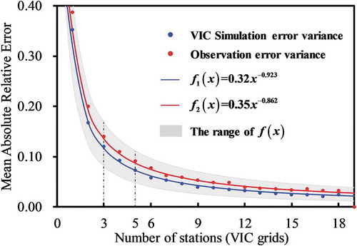
Similarly, a sensitivity analysis in the UHRB for the assimilation ensemble sizes was conducted by comparing the differences between the error variances (R and P_f) derived from all in situ stations (corresponding VIC grids) and a randomly different number of stations (corresponding to VIC grids). As shown in Fig. 15, a sample size of about 3–5 can well hold the error variance information with a MARE of about 0.1. The ensemble sensitivities of the VIC simulation and observation error variance were quite similar within a limited range. This is consistent with the finding shown in Fig. 4 that the representativeness of the point observations and grid simulations is similar over large scales. This finding also provided strong evidence that such a sample size is stable and feasible for our SM assimilation scheme. Moreover, the actual representative error was lower than the results presented in Fig. 15, since it decreases with the radius (Wu et al. 2018) and the sample radius is smaller than the basin radius. In addition, the number of SM stations in the UHRB is increasing, with more than 40 stations since 2016, and this SM assimilation scheme will be more powerful based on future data.

Figure 4. Time-averaged weighting factors (dots) for the study period at different ensemble radius, S₀, which were fitted with a negative exponential function (solid lines).

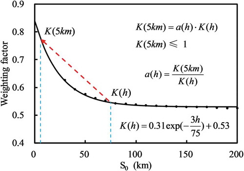
Figure 5. Differences between assimilation gains (ΔG, dots) at different distances, which were fitted with a Gaussian function (solid lines). The normalized weight function is also shown.

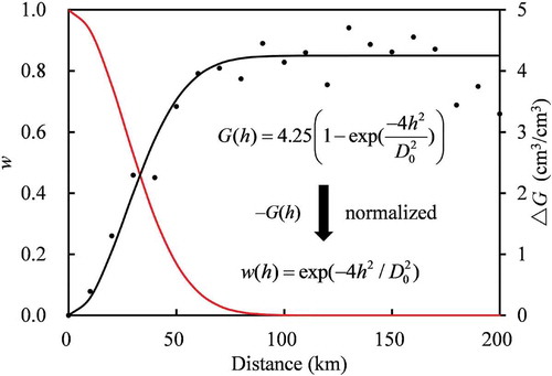
Figure 6. Variograms of (a) the mean value and (b) the standard deviation derived from the in situ SM series. Dots are the experimental semi-variances and the solid lines show the fitted model.

Figure 7. Comparison of the simulated and observed daily streamflow at Wangjiaba station for the calibration and validation periods. The Nash-Sutcliffe coefficient (E_c) and relative error (E_r) are also shown.

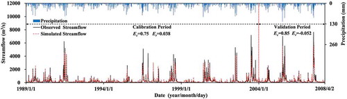
Figure 8. Time series of the in situ observed VIC simulated and assimilated SM (0–10 cm) at three typical stations, (a) SSK, (b) MW and (c) BS for the period January 2012 to December 2014 in the UHRB.

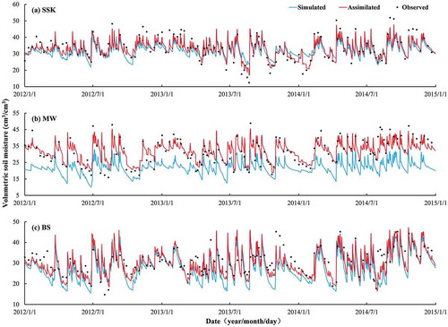
Figure 9. Example of the spatial distribution of (a) observed, (b) VIC simulated and (c) assimilated SM (0–10 cm) values in the UHRB for 11 September 2014.

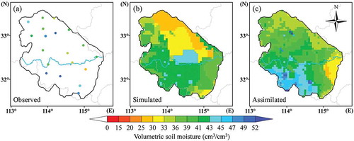
Figure 10. Scatterplots of the simulated and assimilated SM values versus the observed SM values in the UHRB for 11 September 2014.

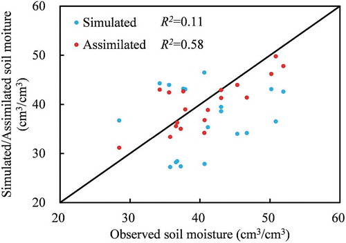
Figure 11. Comparison of (a) correlation coefficient, (b) ubRMSE and (c) Bias for the cross-validated SM series (0–10 cm).

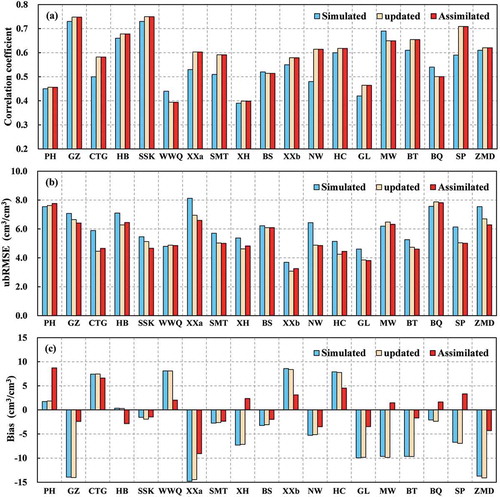
Figure 12. Influence of the SM assimilation on the ET values.

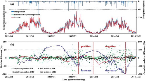
Figure 13. Influence of the SM assimilation on streamflow prediction.

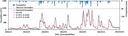
Figure 14. Comparison between monthly streamflow in 2014 and historical monthly streamflow at Wangjiaba station along with corresponding monthly space-averaged precipitation in the UHRB.

Figure 15. Sensitivity analysis of the assimilation ensemble sizes in the UHRB: difference between error variances derived from all in situ stations (corresponding VIC grids) and randomly different number of stations (corresponding VIC grids). Dots represent the average relationship between the MARE and number of stations (corresponding VIC grids), the solid lines represent the fitted empirical model.

5 Summary and conclusions

The objective of this study was to assimilate accurate but sparse in situ SM observations into a continuous hydrological model to improve the SM modelling capacity. Therefore, a regional SM assimilation scheme based on an empirical approach was constructed for this purpose. SM observations for the study period January 2012 to December 2014 were collected from 19 in situ stations in the UHRB. The daily VIC model was built for the UHRB to simulate SM during the study period with a spatial resolution of 5 km × 5 km.

Consideration of spatial variability and regional assimilation are the two main steps in the assimilation scheme. In the first step, the simulation and observation variance were used to represent the spatial variability and simulation error, which were quantified by a weighting factor. In the second step, the assimilation gain interpolation method was employed for the lateral propagation of assimilation effects based on an empirical error weight function. To conduct the SM assimilation scheme, the first-order moment rescaling was used as an a priori processing step for rescaling the observations to the model scale. The data assimilation was then conducted at the simulation scale and the assimilation updated SM was produced. Afterwards, the bias correction based on the first and second-order moments was used as an a posteriori processing step for correcting the assimilation updated SM to obtain the final assimilated SM. The two moments used in the bias correction were derived from the in situ observations by applying the ordinary kriging technique.

Through synthetic assimilation experiments and validations against in situ observations, the assimilated SM was evaluated, and the assimilation feedback on the ET and streamflow was analysed and discussed. The results show that the assimilation scheme can significantly improve SM simulations, and the assimilated SM values showed greater correspondence with the in situ observations compared to the VIC simulations, both spatially and temporally. The assimilation scheme is shown to be capable of combing accurate but sparse in situ observations and continuous VIC simulations. Additionally, the assimilation of in situ observations can continuously affect ET values, and improvements in the SM simulations may be further translated into improved runoff predictions. The SM assimilation scheme forms an important reference for the efficient use of in situ observations, and provides a potential way to improve SM and streamflow simulations. Besides, there is scope for further research on the joint assimilation of in situ observations and temporal continuous satellite SM data, and the further consideration of temporal propagated SM error information.

Disclosure statement

No potential conflict of interest was reported by the authors.

Additional information

Funding

This work is supported by the National Key Research and Development Programme of China [Grant no. 2017YFC1502403]; the National Natural Science Foundation of China [Grant nos. 51579065 and 51779071]; the Fundamental Research Funds for the Central Universities [Grant no. 2017B10514] and the Central Public-interest Scientific Institution Basal Research Fund [Grant no. HKY-JBYW-2017-12].

References

- Alvarez-Garreton, C., et al., 2015. Improving operational flood ensemble prediction by the assimilation of satellite soil moisture: comparison between lumped and semi-distributed schemes. Hydrology and Earth System Sciences, 19 (4), 1659–1676. doi:10.5194/hess-19-1659-2015
- Aubert, D., Loumagne, C., and Oudin, L., 2003. Sequential assimilation of soil moisture and streamflow data in a conceptual rainfall-runoff model. Journal of Hydrology, 280 (1–4), 145–161. doi:10.1016/s0022-1694(03)00229-4
- Boone, A., et al., 2004. The Rhone-aggregation land surface scheme intercomparison project: an overview. Journal of Climate, 17 (1), 187–208. doi:10.1175/1520-0442(2004)017<0187:trlssi>2.0.co;2
- Brocca, L., et al., 2010. ASCAT soil wetness index validation through in situ and modeled soil moisture data in central Italy. Remote Sensing of Environment, 114 (11), 2745–2755. doi:10.1016/j.rse.2010.06.009
- Brocca, L., et al., 2011. Soil moisture estimation through ASCAT and AMSR-E sensors: an intercomparison and validation study across Europe. Remote Sensing of Environment, 115 (12), 3390–3408. doi:10.1016/j.rse.2011.08.003
- Chen, F., et al., 2011a. Improving hydrologic predictions of a catchment model via assimilation of surface soil moisture. Advances in Water Resources, 34 (4), 526–536. doi:10.1016/j.advwatres.2011.01.011
- Chen, Y., et al., 2011b. Liuxihe model and its modeling to river basin flood. Journal of Hydrologic Engineering, 16 (1), 33–50. doi:10.1061/(ASCE)HE.1943-5584.0000286
- Chen, Y., Li, J., and Xu, H., 2016. Improving flood forecasting capability of physically based distributed hydrological models by parameter optimization. Hydrology and Earth System Sciences, 20, 375–392. doi:10.5194/hess-20-375-2016
- Crow, W.T., et al., 2012. Upscaling sparse ground-based soil moisture observations for the validation of coarse-resolution satellite soil moisture products. Reviews of Geophysics, 50. doi:10.1029/2011rg000372
- Crow, W.T. and van den Berg, M.J., 2010. An improved approach for estimating observation and model error parameters in soil moisture data assimilation. Water Resources Research, 46. doi:10.1029/2010wr009402
- De Lannoy, G.J.M., et al., 2007. Correcting for forecast bias in soil moisture assimilation with the ensemble Kalman filter. Water Resources Research, 43 (9). doi:10.1029/2006wr005449
- de Rosnay, P., et al., 2013. A simplified extended Kalman filter for the global operational soil moisture analysis at ECMWF. Quarterly Journal of the Royal Meteorological Society, 139 (674), 1199–1213. doi:10.1002/qj.2023
- Dorigo, W.A., et al., 2010. Error characterisation of global active and passive microwave soil moisture datasets. Hydrology and Earth System Sciences, 14 (12), 2605–2616. doi:10.5194/hess-14-2605-2010
- Dorigo, W.A., et al., 2015. Evaluation of the ESA CCI soil moisture product using ground-based observations. Remote Sensing of Environment, 162, 380–395. doi:10.1016/j.rse.2014.07.023
- Draper, C., et al., 2011. Assimilation of ASCAT near-surface soil moisture into the SIM hydrological model over France. Hydrology and Earth System Sciences, 15 (12), 3829–3841. doi:10.5194/hess-15-3829-2011
- Draper, C.S., et al., 2012. Assimilation of passive and active microwave soil moisture retrievals. Geophysical Research Letters, 39 (4), 127–145. doi:10.1029/2011GL050655
- Drusch, M., Wood, E.F., and Gao, H., 2005. Observation operators for the direct assimilation of TRMM microwave imager retrieved soil moisture. Geophysical Research Letters, 32 (15). doi:10.1029/2005gl023623
- Du, E., Di Vittorio, A., and Collins, W.D., 2016. Evaluation of hydrologic components of community land model 4 and bias identification. International Journal of Applied Earth Observation and Geoinformation, 48, 5–16. doi:10.1016/j.jag.2015.03.013
- Dumedah, G. and Coulibaly, P., 2013. Evolutionary assimilation of streamflow in distributed hydrologic modeling using in-situ soil moisture data. Advances in Water Resources, 53, 231–241. doi:10.1016/j.advwatres.2012.07.012
- Dumedah, G. and Walker, J.P., 2014. Intercomparison of the JULES and CABLE land surface models through assimilation of remotely sensed soil moisture in southeast Australia. Advances in Water Resources, 74, 231–244. doi:10.1016/j.advwatres.2014.09.011
- Enenkel, M., et al., 2016. Combining satellite observations to develop a global soil moisture product for near-real-time applications. Hydrology and Earth System Sciences, 20 (10), 4191–4208. doi:10.5194/hess-20-4191-2016
- Escorihuela, M.J., et al., 2010. Effective soil moisture sampling depth of L-band radiometry: a case study. Remote Sensing of Environment, 114 (5), 995–1001. doi:10.1016/j.rse.2009.12.011
- Evensen, G., 1994. Sequential data assimilation with a nonlinear quasi‐geostrophic model using Monte Carlo methods to forecast error statistics. Journal of Geophysical Research Atmospheres, 99 (C5), 10143–10162. doi:10.1029/94JC00572
- Evensen, G., 2003. The ensemble Kalman filter: theoretical formulation and practical implementation. Ocean Dynamics, 53 (4), 343–367. doi:10.1007/s10236-003-0036-9
- Fairbairn, D., et al., 2015. Comparing the ensemble and extended Kalman filters for in situ soil moisture assimilation with contrasting conditions. Hydrology and Earth System Sciences, 19 (12), 4811–4830. doi:10.5194/hess-19-4811-2015
- Fang, X., Xu, Y., and Zhou, Z., 2011. New correlations of single-phase friction factor for turbulent pipe flow and evaluation of existing single-phase friction factor correlations. Nuclear Engineering and Design, 241 (3), 897–902. doi:10.1016/j.nucengdes.2010.12.019
- Ford, T., Harris, E., and Quiring, S., 2014. Estimating root zone soil moisture using near-surface observations from SMOS. Hydrology and Earth System Sciences, 18 (1), 139–154. doi:10.5194/hess-18-139-2014
- Gao, H., et al., 2006. Using TRMM/TMI to retrieve surface soil moisture over the southern United States from 1998 to 2002. Journal of Hydrometeorology, 7 (1), 23–38. doi:10.1175/jhm473.1
- Gao, S., et al., 2014. Estimating the spatial distribution of soil moisture based on Bayesian maximum entropy method with auxiliary data from remote sensing. International Journal of Applied Earth Observation and Geoinformation, 32, 54–66. doi:10.1016/j.jag.2014.03.003
- Gruber, A., Crow, W.T., and Dorigo, W.A., 2018. Assimilation of spatially sparse in situ soil moisture networks into a continuous model domain. Water Resources Research, 54, 1353–1367. doi:10.1002/2017WR021277
- Gruhier, C., et al., 2010. Soil moisture active and passive microwave products: intercomparison and evaluation over a Sahelian site. Hydrology and Earth System Sciences, 14 (1), 141–156. doi:10.5194/hess-14-141-2010
- Han, E., Merwade, V., and Heathman, G.C., 2012. Implementation of surface soil moisture data assimilation with watershed scale distributed hydrological model. Journal of Hydrology, 416, 98–117. doi:10.1016/j.jhydrol.2011.11.039
- Hansen, M.C., et al., 2000. Global land cover classification at 1km spatial resolution using a classification tree approach. International Journal of Remote Sensing, 21 (6–7), 1331–1364. doi:10.1080/014311600210209
- Jia, Y., et al., 2001. Development of WEP model and its application to an urban watershed. Hydrological Processes, 15 (11), 2175–2194. doi:10.1002/hyp.275
- Kolassa, J., Reichle, R.H., and Draper, C.S., 2017. Merging active and passive microwave observations in soil moisture data assimilation. Remote Sensing of Environment, 191, 117–130. doi:10.1016/j.rse.2017.01.015
- Kumar, S.V., et al., 2012. A comparison of methods for a priori bias correction in soil moisture data assimilation. Water Resources Research, 48. doi:10.1029/2010wr010261
- Laiolo, P., et al., 2016. Impact of different satellite soil moisture products on the predictions of a continuous distributed hydrological model. International Journal of Applied Earth Observation and Geoinformation, 48, 131–145. doi:10.1016/j.jag.2015.06.002
- Lakhankar, T., et al., 2010. Analysis of large scale spatial variability of soil moisture using a geostatistical method. Sensors, 10 (1), 913–932. doi:10.3390/s100100913
- Liang, X., et al., 1994. A simple hydrologically based model of land surface water and energy fluxes for general circulation models. Journal of Geophysical Research: Atmospheres, 99 (D7), 14415–14428. doi:10.1029/94JD00483
- Liang, X., Wood, E.F., and Lettenmaier, D.P., 1996. Surface soil moisture parameterization of the VIC-2L model: evaluation and modification. Global and Planetary Change, 13 (1–4), 195–206. doi:10.1016/0921-8181(95)00046-1
- Lievens, H., et al., 2015. SMOS soil moisture assimilation for improved hydrologic simulation in the Murray Darling Basin, Australia. Remote Sensing of Environment, 168, 146–162. doi:10.1016/j.rse.2015.06.025
- Liu, Y., et al., 2012. Advancing data assimilation in operational hydrologic forecasting: progresses, challenges, and emerging opportunities. Hydrology and Earth System Sciences, 16 (10), 3863–3887. doi:10.5194/hess-16-3863-2012
- Liu, Y.Y., et al., 2011. Developing an improved soil moisture dataset by blending passive and active microwave satellite-based retrievals. Hydrology and Earth System Sciences, 15 (2), 425–436. doi:10.5194/hess-15-425-2011
- Mao, Y., et al., 2017. Spatio-temporal analysis of drought in a typical plain region based on the soil moisture anomaly percentage index. Science of the Total Environment, 576, 752–765. doi:10.1016/j.scitotenv.2016.10.116
- Mao, Y.X., et al., 2019. A framework for diagnosing factors degrading the streamflow performance of a soil moisture data assimilation system. Journal of Hydrometeorology, 20 (1), 79–97. doi:10.1175/JHM-D-18-0115.1
- Martens, B., et al., 2016. Improving terrestrial evaporation estimates over continental Australia through assimilation of SMOS soil moisture. International Journal of Applied Earth Observation and Geoinformation, 48, 146–162. doi:10.1016/j.jag.2015.09.012
- Massari, C., et al., 2015. Data assimilation of satellite soil moisture into rainfall-runoff modelling: a complex recipe? Remote Sensing, 7 (9), 11403–11433. doi:10.3390/rs70911403
- Mo, K.C. and Lettenmaier, D.P., 2014. Objective drought classification using multiple land surface models. Journal of Hydrometeorology, 15 (3), 990–1010. doi:10.1175/jhm-d-13-071.1
- Nash, J.E. and Sutcliffe, J.V., 1970. River flow forecasting through conceptual models part I — a discussion of principles. Journal of Hydrology, 10 (3), 282–290. doi:10.1016/0022-1694(70)90255-6
- Penna, D., et al., 2009. Hillslope scale soil moisture variability in a steep alpine terrain. Journal of Hydrology, 364 (3–4), 311–327. doi:10.1016/j.jhydrol.2008.11.009
- Penna, D., et al., 2013. Soil moisture temporal stability at different depths on two alpine hillslopes during wet and dry periods. Journal of Hydrology, 477, 55–71. doi:10.1016/j.jhydrol.2012.10.052
- Peters-Lidard, C.D., et al., 2011. Estimating evapotranspiration with land data assimilation systems. Hydrological Processes, 25 (26), 3979–3992. doi:10.1002/hyp.8387
- Reichle, R.H. and Koster, R.D., 2004. Bias reduction in short records of satellite soil moisture. Geophysical Research Letters, 31 (19). doi:10.1029/2004gl020938
- Reichle, R.H., Mclaughlin, D.B., and Entekhabi, D., 2002. Hydrologic data assimilation with the ensemble Kalman filter. Monthly Weather Review, 130 (1), 103–114. doi:10.1175/1520-0493(2002)130<0103:HDAWTE>2.0.CO;2
- Reynolds, C.A., Jackson, T.J., and Rawls, W.J., 2000. Estimating soil water-holding capacities by linking the Food and Agriculture Organization soil map of the world with global pedon databases and continuous pedotransfer functions. Water Resources Research, 36 (12), 3653–3662. doi:10.1029/2000wr900130
- Rosenbrock, H.H., 1960. An automatic method for finding the greatest or least value of a function. The Computer Journal, 3 (3), 175–184. doi:10.1093/comjnl/3.3.175
- Sahoo, A.K., et al., 2013. Assimilation and downscaling of satellite observed soil moisture over the little river experimental watershed in Georgia, USA. Advances in Water Resources, 52, 19–33. doi:10.1016/j.advwatres.2012.08.007
- Seneviratne, S.I., et al., 2010. Investigating soil moisture-climate interactions in a changing climate: a review. Earth-Science Reviews, 99 (3–4), 125–161. doi:10.1016/j.earscirev.2010.02.004
- Shao, J., 1993. Linear model selection by cross-validation. Publications of the American Statistical Association, 88 (422), 486–494. doi:10.1080/01621459.1993.10476299
- Shi, C., et al., 2011. China land soil moisture EnKF data assimilation based on satellite remote sensing data. Science China-Earth Sciences, 54 (9), 1430–1440. doi:10.1007/s11430-010-4160-3
- Sun, Y., et al., 2017. Preliminary evaluation of the SMAP radiometer soil moisture product over china using in situ data. Remote Sensing, 9 (3). doi:10.3390/rs9030292
- Tramblay, Y., et al., 2011. Impact of rainfall spatial distribution on rainfall-runoff modelling efficiency and initial soil moisture conditions estimation. Natural Hazards and Earth System Sciences, 11 (1), 157–170. doi:10.5194/nhess-11-157-2011
- Walker, J.P., Willgoose, G.R., and Kalma, J.D., 2001. One-dimensional soil moisture profile retrieval by assimilation of near-surface measurements: a simplified soil moisture model and field application. Journal of Hydrometeorology, 2 (4), 356–373. doi:10.1175/1525-7541(2001)002<0356:odsmpr>2.0.co;2
- Wu, Z., et al., 2007. Thirty-five year (1971–2005) simulation of daily soil moisture using the variable infiltration capacity model over China. Atmosphere-Ocean, 45 (1), 37–45. doi:10.3137/ao.v450103
- Wu, Z.Y., et al., 2011. Reconstructing and analyzing China’s fifty-nine year (1951–2009) drought history using hydrological model simulation. Hydrology and Earth System Sciences, 15 (9), 2881–2894. doi:10.5194/hess-15-2881-2011
- Wu, Z.Y., et al., 2018. An advanced error correction methodology for merging in-situ observed and model-based soil moisture. Journal of Hydrology, 566 (2018), 150–163. doi:10.1016/j.jhydrol.2018.09.018
- Yamamoto, J.K., 2005. Correcting the smoothing effect of ordinary kriging estimates. Mathematical Geology, 37 (1), 69–94. doi:10.1007/s11004-005-8748-7
- Yang, Y., Shang, S., and Chao, L.I., 2010. Correcting the smoothing effect of ordinary Kriging estimates in soil moisture interpolation. Advances in Water Science, 21 (2), 208–213. doi:10.14042/j.cnki.32.1309.2010.02.018
- Yilmaz, M.T., et al., 2012. An objective methodology for merging satellite- and model-based soil moisture products. Water Resources Research, 48 (11). doi:10.1029/2011wr011682
- Zhang, S., et al., 2016. Hydrological change driven by human activities and climate variation and its spatial variability in Huaihe Basin, China. Hydrological Sciences Journal-Journal Des Sciences Hydrologiques, 61 (8), 1370–1382. doi:10.1080/02626667.2015.1035657
- Zou, L., et al., 2017. Implementation of evapotranspiration data assimilation with catchment scale distributed hydrological model via an ensemble Kalman filter. Journal of Hydrology, 549, 685–702. doi:10.1016/j.jhydrol.2017.04.036