Comparative analysis of nonparametric change-point detectors commonly used in hydrology

ABSTRACT

Several commonly-used nonparametric change-point detection methods are analysed in terms of power, ability and accuracy of the estimated change-point location. The analysis is performed with synthetic data for different sample sizes, two types of change and different magnitudes of change. The methods studied are the Pettitt method, a method based on the Cramér von Mises (CvM) two-sample test statistic and a variant of the CUSUM method. The methods differ considerably in behaviour. For all methods the spread of estimated change-point location increases significantly for points near one of the ends of the sample. Series of annual maximum runoff for four stations on the Yangtze River in China are used to examine the performance of the methods on real data. It was found that the CvM-based test gave the best results, but all three methods suffer from bias and low detection rates for change points near the ends of the series.

KEYWORDS:

• change-point detection
• Pettitt test
• Cramér von Mises test
• CUSUM test
• power
• ability
• uncertainty

Editor A. Castellarin Associate editor A. Langousis

1 Introduction

Today environmental scientists are well aware of the changes that affect the systems they study. Changes in land use, increasing urbanization and climate change combine to complicate the process of predicting the future behaviour of these systems (Kundzewicz 2011, Montanari et al. 2013, McMillan et al. 2016). These predictions are needed to answer practical questions like “How high should this dam be to be functional for 50 years?” or “Can we safely develop this coastal area?”. Given the inherent uncertainty about the future, predictions inevitably involve statistics, for instance, the probability of certain amounts of precipitation or runoff. These statistics may or may not be influenced by changes in the environment.

One type of change one may look for is a change point (Pettitt 1979, Gao et al. 2010), a moment in time where there is an abrupt change in one or more of the properties of the time series such as the mean, the median, or the standard deviation.

The art of finding change points was studied first to detect changes in product quality in manufacturing (Dudding and Jennett 1942, p. 1954). One of the earliest papers that addressed this question by developing and using a formal statistical test in a hydrological context was written by McGilchrist and Woodyer (1975). They looked for change points in an 88-year-long series of yearly rainfall at Walgett, New South Wales, Australia.

Change-point analysis was initially restricted to univariate time series of independent variables under the assumption of “At Most One Change” (AMOC). It was extended to series with multiple change points (Lebarbier 2005, Lavielle and Teyssiere 2006) and to multivariate time series (Matteson and James 2014). New methods were developed to consider dependence within a series, or high-dimensional multivariate time series (Ray and Tsay 2002, Berkes et al. 2006, Lund et al. 2007, Gombay 2008, Shao and Zhang 2010, Xie et al. 2012, Shao 2015, Cho and Fryzlewicz 2015, Zhang and Lavitas 2018). Detecting change points in a series with trend was studied by analysing a two-phase regression model, see for example Lund et al. (2007), Wang (2003) and Beaulieu et al. (2012).

Hydrological processes are widely thought to have changing properties (Thirel et al. 2015, Hajani et al. 2017, Sa’adi et al. 2017). Many types of human intervention may result in change points in hydrological time series, for instance, construction of dams, changes in instrumentation or measurement protocol and relocation of measurement stations.

Sometimes the potential cause of a change point in a time series is known, for example, the relocation of a measurement station. These are referred to as “documented change points”, where detected change points can be examined in context. But on other occasions, there are no explicitly documented potential causes for change points and only the outcome of the statistical change point analysis can be used to judge the reliability of the result (Lund and Reeves 2002, Menne and Williams Jr 2005, Reeves et al. 2007, Wang 2008).

As in other areas of statistics, there are parametric and non-parametric (distribution free) methods for change-point detection. Parametric methods assume that observations are from a known parametrized family of distributions. A number of classical parametric methods have been developed, see for example Chernoff and Zacks (1964), Kander and Zacks (1966), Hawkins (1987), or Gurevich and Vexler (2010). In practice, there is often not enough information on the type of distribution of a hydrological sample to make an informed choice for the distribution family and subsequently perform a parametric change-point detection analysis. Therefore, only nonparametric tests are studied in this paper.

Previous studies have analysed Pettitt’s method in terms of its ability to detect the correct time of change for different distributions (Xie et al. 2014) and sensitivity for the gamma distribution (Mallakpour and Villarini 2016), but comparative studies of multiple methods are rare.

Time series analysis of hydrological data is a complex topic due to dependence in the time series and the complexities of multivariate data. This study considers only one specific context: under ideal circumstances and for a time series containing only one variable, can change-point analysis be used for exploratory data analysis and what are its limitations? Questions to be answered are:

• Can the probability of incorrectly signaling a change point be predicted?

• What is the probability of correctly detecting a change point?

• How close are the estimates to the correct location?

• What is the effect of time series length?

• Is there a relationship between the size of the change and the answers to the above questions?

• Does it matter when our series starts or ends? In other words: is it safe to look at parts of a time series that contain a given range of potential change points, but have different start or end years?

The following change-point detection methods are considered: the method described in Pettitt (1979), which we refer to as “Pet-CP”, a method based on the two-sample Cramér von Mises test statistic, which we refer to as “CvM-CP” (Holmes et al. 2013, Xiong et al. 2015), and a method based on CUSUM median statistics, which we refer to as “CUSUM-CP” (McGilchrist and Woodyer 1975, Chiew and McMahon 1993, Rahman et al. 2018). Xiong et al. (2015) used CvM-CP to detect the change point in multivariate time series, but this paper applies CvM-CP in the univariate situation.

2 Methodology and data

This study contains two groups of experiments. The first experiment uses synthetic data series to examine how well the methods perform. The second experiment takes four time series of the maximum runoff observed in a given year and uses the methods to look for change points in the full series and subseries for different start and/or end years.

From a statistical point of view, a time series of hydrological measurements of length n can be seen as a vector of n observations (x₁, x₂, …, x_n) corresponding to one sample of a random vector (X₁, X₂, …, X_n). The vector components may or may not be independent, and they may or may not have the same marginal distribution. The methods for change point analysis used in this study has three components:

• a test statistic;

• an exact (or approximate) distribution of the test statistic under the null hypothesis; and

• an estimator $\hat{\tau }$ for the point in time τ where the change occurs (the change point).

For these tests the null hypothesis is: There is no change point. To apply one of these methods, first a significance level is set, next the statistic is calculated and, finally, if the null hypothesis is rejected, the estimator $\hat{\tau }$ is applied and the resulting change point location is reported.

All tests given here are described in a form suitable for independent vector components and the presence of at most one change point, so either the n vector components have the same distribution, or the first τ are from one distribution and the remaining n – τ are from a second distribution. If the vector components are not independent, then either adjustment of the distribution of the test statistic, or pre-processing of the time series is indicated (Kundzewicz and Robson 2000), and if there are multiple change points, then the tests need to be extended; both are outside the scope of this paper. Background information on change detection can be found in Kundzewicz and Robson (2000, 2004).

2.1 Change-point detection methods

2.1.1 CvM-CP method

The original Cramér von Mises (CvM) test was intended to determine whether all observations in a sample of n independent observations were drawn from a given probability distribution (Anderson and Darling 1954). A modification can be used to test whether or not two samples were drawn from the same distribution (Anderson 1962). Holmes et al. (2013) developed a method on the basis of the two-sample CvM test statistic to detect the change point within the multivariate series. This was a further development of the approach proposed by Gombay and Horváth (1999). According to Bücher et al. (2014), the method developed by Holmes et al. (2013) performs much better than that based on the two-sample Kolmogorov-Smirnov test statistic. Moreover, it is not only useful in detecting the change point within a univariate time series, but can also be applied to get the marginal distribution of a multivariate hydrological time series, such as copula-based rainfall–runoff multivariate series (Xiong et al. 2015). The notation from (Xiong et al. 2015) is used to describe the CvM-CP detection method. We start by defining:

(1) $\mathbf{1}\left(x\le y\right)=\left\{\begin{array}{c}0:x>y\\ 1:x\le y\end{array}\right.$(1)

which, in the one-dimensional case, is a step function. This is used to define the empirical distribution function for the part of the sample up to a potential change point:

(2) $F_{\tau }\left(X_k\right)=\frac{1}{\tau }{\sum }_{i=1}^{\tau }\mathbf{1}\left(X_i\le X_k\right)$(2)

and the empirical distribution function for the part of a sample after the potential change point:

(3) $F_{n-\tau }^{\ast }\left(X_k\right)=\frac{1}{n-\tau }{\sum }_{i=\tau +1}^n\mathbf{1}\left(X_i\le X_k\right)$(3)

For a time series of one variable, the CvM-CP test statistic is defined in terms of n – 1 two-sample statistics:

(4) $S_{\tau }=\frac{1}{n}{\sum }_{k=1}^n{\left[D\left(\tau ,X_k\right)\right]}^2$(4)

(5) $D\left(\tau ,X_k\right)=\frac{\tau \left(n-\tau \right)}{n^{3/2}}\left(F_{\tau }\left(X_k\right)-F_{n-\tau }^{\ast }\left(X_k\right)\right)$(5)

The CvM-CP statistic is given by:

(6) $S_n=\underset{1\le \tau <n}{max}{S}_{\tau }$(6)

The distribution for this value under the null hypothesis is not known exactly and an asymptotic distribution is not available. It was approximated empirically from a sample of size 10 000 taken from the standard uniform distribution, as in Holmes et al. (2013). If the null hypothesis does not hold, then the estimator for the change-point location is:

(7) $\hat{\tau }=\mathrm{m}\mathrm{i}\mathrm{n}\left(\underset{1\le \tau <n}{\mathrm{a}\mathrm{r}\mathrm{g}\mathrm{m}\mathrm{a}\mathrm{x}}{S}_{\tau }\right)$(7)

The general approach of choosing the lowest index τ if there are multiple equal maxima was proposed in Antoch et al. (1997).

2.1.2 Pet-CP method

The Pettitt test was specifically designed to detect a single change point (Pettitt 1979). To define the statistic, we need:

(8) $\mathrm{s}\mathrm{g}\mathrm{n}\left(x\right)=\left\{\begin{array}{c}-1ifx<0\\ 0ifx=0\\ 1ifx>0\end{array}\right.$(8)

and the following two-sample test statistic:

(9) $U_{\tau }={\sum }_{i=1}^{\tau }{\sum }_{j=\tau +1}^n\mathrm{s}\mathrm{g}\mathrm{n}\left(X_i-X_j\right)$(9)

Note that the sign function can be expressed in terms of the step function:

(10) $\mathrm{s}\mathrm{g}\mathrm{n}\left(X_i-X_j\right)=\mathbf{1}\left(X_j\le X_i\right)-\mathbf{1}\left(X_i\le X_j\right)$(10)

The Pettit test statistic itself is given by:

(11) $K_n=\underset{1\le \tau <n}{max}\left|U_{\tau }\right|$(11)

If the null hypothesis does not hold, then the estimator for the change-point location is:

(12) $\hat{\tau }=\mathrm{m}\mathrm{i}\mathrm{n}\left(\underset{1\le \tau <n}{\mathrm{a}\mathrm{r}\mathrm{g}\mathrm{m}\mathrm{a}\mathrm{x}}{U}_{\tau }\right)$(12)

According to Pettitt (1979), the limit distribution of K_n for large n is given by:

(13) $\mathrm{P}\mathrm{r}\left(K_n\sqrt{\frac{3}{n^2+n^3}}\le a\right)=1+2{\sum }_{j=1}^{\mathrm{\infty }}{\left(-1\right)}^j{\mathrm{e}}^{-2j^2{a}^2}$(13)

where the right-hand side represents the cumulative distribution function (cdf) of the Kolmogorov distribution. Most papers that apply this test use this limit distribution, so it will be used here as well.

2.1.3 CUSUM-CP method

Page (1954) was the first to suggest the use of a cumulative sum to find changes in a parameter of interest. McGilchrist and Woodyer (1975) used it to detect a change point for even sample lengths; this is the variant used in this study. Chiew and McMahon (1993) used this method to detect change in annual flow of Australian rivers.

The test is defined in terms of a one-sample test statistic:

(14) $V_{\tau }={\sum }_{j=1}^{\tau }\left(2\times \mathbf{1}\left(K\le X_j\right)-1\right)$(14)

for each potential change point. In Equation (14), K is a random variable corresponding to one of several quantities. We follow McGilchrist and Woodyer (1975), who used the sample median. The test statistic is:

(15) $T_n=\frac{2}{n}\underset{1\le \tau <n}{max}\left|V_{\tau }\right|$(15)

and the estimator for the change-point location is:

(16) $\hat{\tau }=\mathrm{m}\mathrm{i}\mathrm{n}\left(\underset{1\le \tau <n}{\mathrm{a}\mathrm{r}\mathrm{g}\mathrm{m}\mathrm{a}\mathrm{x}}\left|V_{\tau }\right|\right)$(16)

According to McGilchrist and Woodyer (1975), under the null hypothesis the limit distribution of T_n for large n is the same as that of the Kolmogorov-Smirnov test statistic. It follows that:

(17) $\mathrm{P}\mathrm{r}\left(T_n\sqrt{\frac{n}{4}}<x\right)=1+2{\sum }_{j=1}^{+\mathrm{\infty }}{\left(-1\right)}^j{\mathrm{e}}^{-2j^2{x}^2}$(17)

where the right-hand side represents the cdf of the Kolmogorov distribution. Most papers that apply this test use this limit distribution, so it will be used here as well.

2.2 Criteria used to evaluate the performance of the tests

The first property to be checked is the empirical type I error probability. For a significance level of 5% the test should reject the null hypothesis, H₀, “There is no change point”, for 5% of the synthetic time series without change point.

To see how well the tests do when detecting change points, we want to approximate the power of the test, which is defined as the probability that a test correctly rejects H₀ without considering the accuracy of the estimate of the change point (Reich et al. 2012). If, for a set of N samples with a change point, the test rejects N_rej, then the empirical probability of correct rejection is:

(18) $\mathrm{p}\mathrm{o}\mathrm{w}\mathrm{e}\mathrm{r}\approx \frac{N_{\mathrm{r}\mathrm{e}\mathrm{j}}}{N}$(18)

While high power is desirable, it is also important that the estimate of the point in time where the change takes place is accurate. A very strict measure of this is the ability of a change-point detection test. This is defined as the empirical probability that the test will correctly reject the null hypothesis and correctly identify the location of the change point (Xie et al. 2014). If for N_cor out of N samples the null hypothesis is rejected and the change point correctly identified, then this is given by:

(19) $\mathrm{a}\mathrm{b}\mathrm{i}\mathrm{l}\mathrm{i}\mathrm{t}\mathrm{y}\approx \frac{N_{\mathrm{c}\mathrm{o}\mathrm{r}}}{N}$(19)

2.3 Data sources: synthetic and observational

2.3.1 Generation of the synthetic time series

Each synthetic time series consisted of n observations of independent random variables where n = 10, 20, …, 100, 200, 500, 1000. Homogeneous synthetic series were generated by sampling M times from the same distribution and used to determine the rejection rate of the null hypothesis “there is no change point”. Time series with exactly one change point τ, with τ = n/10, 2n/10, …, 9n/10, were generated by sampling from a given distribution type with mean μ_L and standard deviation σ_L for the left-hand part of the series up to and including $X_{\tau }$ and mean μ_R and standard deviation σ_R for the right-hand part of the series. The following notation is used:

(20) $\mathrm{\Delta }\mu ={\mu }_{\mathrm{R}}-{\mu }_{\mathrm{L}};\mathrm{\Delta }\sigma ={\sigma }_{\mathrm{R}}-{\sigma }_{\mathrm{L}}$(20)

To study the sensitivity to a change in the mean, series were generated with μ_L = 0, σ_L = σ_R = 1 and μ_R = 0.5, 1, 2, 4, 8. To study the sensitivity to a change in the standard deviation, series were generated with μ_L = μ_R = 0, σ_L = 1 and σ_R = 0.5, 2, 4, 8.

To allow statistical analysis of the results for each specific combination of type of distribution, Δμ, Δσ, change point location τ, and series length n, we generated M synthetic time series. For most combinations, M was equal to 10 000, except for CvM-CP in the case of series of length 200 and 500, where M = 1000 was used, and sample length of 1000, where M = 5000 was used, as CvM-CP turned out to be much more expensive to calculate for long series than the other tests.

2.3.2 Type of distribution

The following four distribution types are considered:

• normal distribution;

• generalized extreme value (GEV) distribution with shape – 0.15, which corresponds to the three-parameter reverse Weibull distribution with shape 20/3;

• GEV distribution with shape 0, which corresponds to the Gumbel distribution; and

• GEV distribution with shape 0.15, which corresponds to the three-parameter Fréchet distribution with shape 20/3. The value 0.15 was chosen as representative for thick-tailed GEV distributions (Koutsoyiannis 2004).

Formulas for the GEV can be found in, for instance, van Nooijen and Kolechkina (2012). Appendix A provides arguments to limit the number of different parameter combinations in case of location–scale distribution families such as those given above.

2.3.3 Source of the real-world data

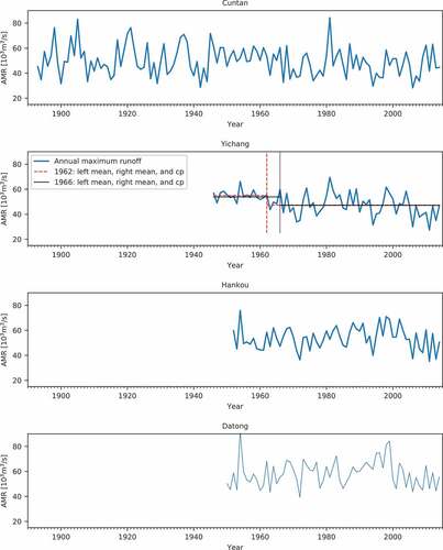
For a given location, the first and last year of a period for which suitable data is available may depend on preprocessing, willingness to allow for missing data and access to recent data. This raises the question whether or not change-point detection results depend on the choice of first and last year. To examine this in the context of real data, measurements from the Yangtze River in China were used. The methods were applied to annual maximum runoff (AMR) observations from four gauge stations: Cuntan (1893–2014), Yichang (1946–2014), Hankou (1952–2014) and Datong (1950-2014) collected by the Ministry of Water Resources of the People’s Republic of China (1919-2014, 1950-2014). The locations of the measurement stations are shown in Fig. 1 and the four AMR time series used are shown in Fig. 2.

Figure 1. Locations of four gauge stations and three dams on the Yangtze river used in the study.

Figure 2. Annual maximum runoff of the four hydrological stations on the Yangtze river.

Over the last 70 years, the Yangtze River basin has been subject to large-scale human intervention (Wang et al. 2013). Reservoir construction has resulted in the building of over 10 000 dams since the 1960s (Yang et al. 2003). Information on the largest two dams in the Yangzte and one in its Hanjiang tributary is given in Table 1 (locations are shown in Fig. 1).

Table 1. Details on some of the dams on the Yangtze river and its tributary.

Dam name	Location	Construction time	Capacity	Reservoir capacity	Location
Danjiangkou	111°29′17″E, 32°33′22″N	1958–1973	900 MW	17.45 km^3	In Han River upstream of Hankou
Gezhouba	111°16′20″E, 30°44′23″N	1970–1988	2715 MW	1.58 km^3	6 km upstream of Yichang
Three Gorges	111°00′12″E, 30°49′23″N	1993–2009	22500 MW	39.3 km^3	44 km upstream of Yichang

For the Yichang, Hankou and Datong series, previous investigations suggest the series can be treated as uncorrelated (Xiong and Guo 2004, Zhang et al. 2006) at the 5% significance level. Zhang et al. (2012) used detrended fluctuation analysis to find the long-range correlation of three datasets from the Yangtze River and concluded that the daily streamflow (1893–2009) from Cuntan station showed no significant correlation.

3 Analysis of the performance of the tests for different input data

The results of the experiments with synthetic data are followed by the results of the experiments on the time series of observed annual maximum flows.

3.1 Synthetic experiment

3.1.1 No change point present

For all tests the significance level was set to 0.05. In other words, it is allowed to incorrectly assume the existence of a change point in 5% of all applications of the test. If the real rejection rate of the null hypothesis “there is no change-point” is higher than this value, then change points will appear more likely than they are in reality, possibly leading to unnecessary efforts to allow for non-existent change. If the real rejection rate of the null hypothesis is lower than this value, then change points will appear less likely than they are in reality, possibly leading to a failure to allow for real change.

Figure 3 shows the rejection rates for the different methods and distributions as a function of sample size.

Figure 3. Rejection rate of H₀ as a function of sample size for each of the tests (significance level α = 0.05). For sample lengths of 1000 and 5000, Monte Carlo simulations are applied for the CvM test.

We can see that Pet-CP and CUSUM-CP start well below the expected rejection rate, while CvM-CP stays close to the chosen significance level. Given that the CvM-CP rejection rate was determined from an empirical distribution, it is not surprising that it does so well; for the other tests we used a limit distribution to approximate the quantile. It is clear that for small samples (n ≤ 100) the limit distributions are not sufficiently accurate, and use of either the exact distribution or an empirical distribution would be preferable. The traditional statistical remedy “use a larger sample” is not an option for time series of extreme values where longer series are simply not available. An alternative traditional remedy for this problem, “use an improved approximation of the distribution”, is simple in theory, but complicated in practice because calculation of the exact distribution, or alternatively the generation of an approximate distribution by Monte Carlo methods can be quite expensive.

3.1.2 One change point present

3.1.2.1 Sensitivity to a change in the mean

The power and ability to correctly identify the change point are shown in Figs. 4 and 5, respectively.

Figure 4. Power of all tests for a change in the mean (n = 100).

Figure 5. Ability of all the tests for a change in the mean (n = 100).

We can see that for all tests both power and ability increase considerably with an increase in the magnitude of the change Δμ in the mean. The plots of power vs the location of the actual change point τ are nearly symmetrical with respect to a vertical line at τ = n/2. For Pet-CP and CvM-CP the power is higher than for CUSUM-CP when Δμ ≤ 1, except for GEV with k = 0.15 (see the bottom row in Fig. 4). For Δμ ≥ 2, all tests have 100% power for τ = 20, 30, …, 80. If we look at the ability as a function of the location of the change point, then for Pet-CP and CvM-CP the function is nearly symmetrical with respect to a vertical line at τ = n/2, and the highest abilities are reached when the actual change point is near n/2. From Figs. 4 and 5, it is clear that the power and ability vary with location for each test; the ability tends to be more sensitive to the magnitude of the change and the location of the change point. For instance, for Pet-CP, when the magnitude of change is the same, the ability (Fig. 5, row 1, column 1) varies much more than the power (Fig. 4, row 1, column 1). The differences in shape indicates the ability of Pet-CP is much more sensitive to location of a change point than the power.

For all three methods, the abilities increase as |Δμ| increases and stabilize for |Δμ| ≥ 4. When τ is near the middle of the series, the ability increases from less than 10% to nearly 100% for increasing |Δμ|. When τ is near the ends of the series, the abilities stay well below 100%. For a series of length 100, detecting a change in the first or last 20 elements of the series, there is a low probability of it being estimated correctly, regardless of the size of the change.

3.1.2.2 Sensitivity to a change in the standard deviation

The results for power (Fig. 6) and ability (Fig. 7) show that Pet-CP and CUSUM-CP cannot detect a change in the standard deviation.

Figure 6. Power of all the tests for a change in the standard deviation (n = 100).

Figure 7. Ability of all the tests for a change in the standard deviation (n = 100).

While CvM-CP can detect a change in the standard deviation, its ability to do so is much lower than in the case of a change in the mean. For a change of a factor of two in the standard deviation, the power is low as well (see the first two columns in both Figs. 6 and 7). The power and ability plots of CvM-CP are nearly symmetrical with respect to a vertical line at τ = n/2, and they reach their highest point when the actual change point is located near n/2. From the first two columns in Fig. 7, the abilities of Pet-CP and CUSUM-CP stay below 1%. The CvM-CP method shows similar abilities for change points at locations τ and n – τ. For τ = 10 and τ = 90, its ability is near zero (see the last column in Fig. 7). It seems that only for very large changes in standard deviation (Δσ ≥ 6) and only for the change points τ = 40–60 near the midpoint of the series does the ability rise above 50% (Fig. 7).

For Pet-CP, the lower sensitivity to a change in σ seems to be known (Talwar and Gentle 1981), but the reasoning behind this is difficult to find. One possible line of reasoning is given in Appendix B. For CUSUM-CP, the original source states that it is intended for detection of changes in the mean, so its failure for the standard deviation was perhaps to be expected.

3.1.2.3 Uncertainty of the estimators for a change in the mean

The ability gives the empirical probability that the estimated change point coincides with the actual change point. In cases where there is a large difference between power and ability, additional information may be needed. The main question in that case is whether the correctly detected, but incorrectly placed change points are clustered near the correct value or not. Results for the normal distribution are presented in Fig. 8. For all tests, the boxplots for change-point estimates when the actual change point is at k or n – k show very similar uncertainty.

Figure 8. Boxplots of the error in the change-point estimates based on 50 000 samples for a change in the mean. The whiskers are at 2.5% and 97.5%; the crosses show the estimates outside that range.

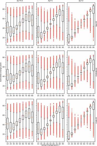
For Δμ = 0.5, the systematic error (bias) near the ends of the series and the spread in the estimate are both too large for practical use. Take CvM-CP for example, and Δμ = 0.5 (Fig. 8, row 3, column 1): for synthetic series of length 100 with a change point at position 10, the boxplot of the estimates has median near 42 and inter-quartile range of about 22. For a change point at position 20, the boxplot of the estimates shows a median near 32 with an interquartile range of about 18. Similar, but negative, biases occur for change points near the end of the series. Similar bias and spread occur for the other methods at Δμ = 0.5.

For Δμ = 1, the systematic error near the ends is still large. Moreover, the 95% confidence interval is large even for the centre point of the series. For Δμ = 2, there are still problems with the systematic error near the end of the series, but in the case of CvM-CP (see the last plot in the last row of Fig. 8, points between position 20 and position 80), the distribution of the spread in the estimates approaches reasonable values.

The results presented here imply that change points near the end of the series, if detected, will almost always result in a relatively large error in the estimated change point.

3.1.2.4 Uncertainty of the estimators for a change in the standard deviation

Results for the normal distribution are presented in Fig. 9. For all tests, the boxplots for change point locations k and n − k show very similar uncertainty. Take for example the row of boxplots for $\hat{\tau }$ as found by Pet-CP in Fig. 9: when τ_true is located at k and n − k, the boxplots for Pet-CP have similar widths and the interquartile distances are close to 20. The wide interquartile ranges indicate considerable uncertainty for the location of changes in the standard deviation.

Figure 9. Boxplots of the error in the change-point estimates based on 50 000 samples for a change in the standard deviation. The whiskers are at 2.5% and 97.5%; the crosses show the estimates outside that range.

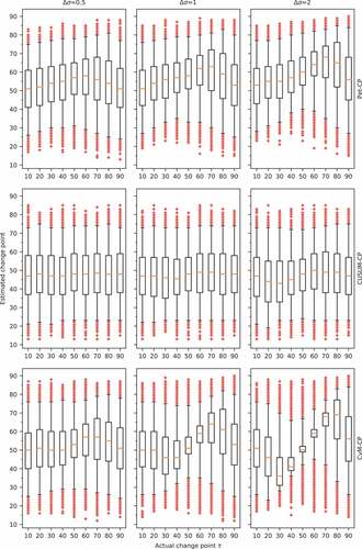
For both Pet-CP and CUSUM-CP, it is clear from the systematic error and the 95% confidence interval that the methods cannot be used to detect a change in standard deviation. The plots in the last row of Fig. 9 show that, for CvM-CP, the results improve with increasing size of the change, but only reach useable levels for the changes Δσ = 2. The spread and bias in the estimated change point locations are illustrated by the boxplot. Only for CvM-CP, Δσ ≥ 2 and τ = 40–60 is there any hope of getting a reliable answer.

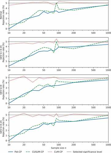
3.1.2.5 Influence of the sample size on ability

For the mean, the ability of the detectors first increases as sample size n increases from 10 to 100 (Fig. 10). When sample size exceeds 100, the ability of the detectors becomes nearly constant, and the ability for n = 1000 is nearly the same as for n = 100. From the first plot in the first row of Fig. 10, for all magnitudes of change, the ability of Pet-CP equals 0 when the sample size is 10. Therefore, when the sample size is 10, Pet-CP is not capable of finding a change point and it is visibly outperformed by CUSUM-CP and CvM-CP.

Figure 10. Ability of the different tests for a change in the mean and standard deviation at the midpoint of the series as a function of sample size n.

Based on the first two plots in the bottom row of Fig. 10, the ability of both Pet-CP and CUSUM-CP stays at very low levels. Accordingly, in the case of Pet-CP and CUSUM-CP, a detection of a shift in the standard deviation is not possible, and the magnitude of Δσ has no significant influence on their ability. For CvM-CP, the ability to detect a change in standard deviation increases considerably as the sample size increases from 30 to 100 (Fig. 10, last row, third column). The ability found for length n = 1000 suggests this increase continues more slowly between n = 100 and n = 1000. Therefore, compared to Pet-CP and CUSUM-CP, CvM-CP is superior in finding a change point in the standard deviation. Considering that the performance of CvM-CP is comparable to that of Pet-CP and CUSUM-CP in detecting a change point in the mean, its better performance in finding a change point in the standard deviation makes CvM-CP much more attractive in change-point detection.

For change points near the start (or end) of the series, both power (Fig. 11) and ability (Fig. 12) decrease with increasing series length. From the power and ability of Pet-CP and CvM-CP shown in the first and third columns of Figs. 11 and 12, their performance in finding a change point located near the start (or end) is very similar and it stays constant till sample length 150; after that their performance decreases rapidly to a relatively low level. But for CUSUM-CP, its power and ability start decreasing when the sample length exceeds 20. For instance, in the middle column of Fig. 11, the power of CUSUM-CP decreases from 100% to 40% when the sample size changes from 20 to 30 for Δμ = 8. From the experiments, we have observed that ability and power for similar relative change point locations, for instance 2n/10, have similar values for different sample sizes. In brief: adding points at the end of a series makes detection of change points at the start of the series less likely. At the same time it makes detection of change points that were near the end before the addition of points at the end more likely.

Figure 11. Power of the different tests for a change in mean at location 10 as a function of sample size n (number of samples M = 1000).

Figure 12. Ability of the different tests for a change in mean at location 10 as a function of sample size n (number of samples M = 1000).

3.2 Application of the tests to historical data for the Yangtze river

3.2.1 Effect of the start and end point of the series

To investigate the influence of the time series length in practice, we took the longest time series corresponding to Cuntan station (Fig. 2) and looked for change points in subseries. The starting year was varied from 1893 to 1957 and the end year from 1964 to 2014. The results are presented in Fig. 13, where a marker at a given pair of years indicates whether or not a change point was found.

Figure 13. Plot of change points found in subseries of the Cuntan data by the three methods. A marker at a given coordinate pair (x,y) indicates whether or not a change point was found for a series starting in year x and ending in year y.

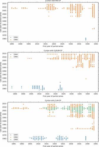
In Fig. 13, the different coloured points denote the different years of significant change for Cuntan station for subseries of years with different start and end years. The bottom plot shows that, depending on which subseries is used, CvM-CP may find three different change points. Comparison of the top and bottom rows shows a similar pattern of detection for subseries ending after 1995 for CvM-CP and Pet-CP. For series ending in 1980, Pet-CP detects 1966 as a change point for more starting years than the other two methods.

For time series with different combinations of start/end year, 1944 and 1966 are found as change points in some subseries by all three methods, but subseries with a significant change point located at 1968 are only found by CvM-CP. It is clear that for all methods the detection and location of a change point depend on the choice of subseries. In other words, different combinations of start/end year will lead to different change-point detection results. The other time series showed similar effects.

As start and end year change, the change point appears, disappears and reappears, possibly in a different year. This is a cause for concern. If two researchers have access to datasets with different start and end points, then they may come to different conclusions about the presence and location of change points. This is particularly unfortunate if, for example, a design decision taken in 2020 on the basis of the absence of a change point in a time series turns out to be invalid in 2030, when the time series – now extended with data for the intervening years – shows a change point in 2010 that invalidates the analysis made in 2020.

Time series of yearly maxima increase in length by one year each year. If this can lead to the appearance or disappearance of change points far from the end of the series, it calls into question the reliability of the results.

3.2.2 Change-point detection

The results of the application of the methods to the entire AMR time series of four gauge stations are as follows: Yichang station is the only one where change points are detected at the 5% significance level (see Fig. 2). For that station Pet-CP and CvM-CP find a change point in 1966 and CUSUM-CP finds one in 1962. The relative changes in mean and standard deviation for the change points are given in Table 2.

Table 2. Change in the mean (μ) and standard deviation (σ) at each detected change point – Yichang station.

Change point	μ (m^3/s)	σ (m^3/s)	μL (m^3/s)	μRμR (m^3/s)	σL (m^3/s)	σR (m^3/s)	Δμ/σ (-)	Δσ/σ (-)
1962	49104	8642	55047	47101	4065	8876	–0.91	0.56
1966			54152	46896	4847	9038	–0.84	0.48

Other studies have also looked for change points in various types of hydrological series in the Yangtze River basin. For example, Xie et al. (2014) applied the Pettitt method and found a change in 1962 in the series of annual maxima at Yichang station for the period 1882–2010, with a p value of 0.0183. They also found a change in 1979 in the series of annual maxima series for 1952–2000 at Hankou station, with a p value of 0.2131. Xiong and Guo (2004) studied the time series of mean annual flows at Yichang station and found a peak in the posterior distribution for the change point in 1968, close to the points found in this study.

None of the methods found a significant change point at a measurement station in the construction period of the dams upstream of that station. For the Three Gorges Dam (TGD) project the non-detection of a change point after the start of construction is in line with the analysis of the Yichang series of annual mean flows for the period 1882–2001 by Xiong and Guo (2004), who found a peak only in the posterior distribution for the change point in 1968. However, this does not necessarily mean there is no change, Xiong and Guo (2004) wrote:

“As the change points for both the annual minimum and the annual mean series occurred before 1993 (the year in which the Three Gorges Project commenced), one can state that, since the construction of the Three Gorges Project there have not been any significant changes in the annual minimum or the annual mean series. However, it is very possible that the above conclusions might change with time, as the Three Gorges Project will definitely exert some influences on the flow regime of the Yangtze River at the Yichang hydrological station. Any change in the characteristics of the hydrological time series of Yichang station in the future could be a reason for modifying the initial construction and operation plan for the Three Gorges Project.”

Our results for Yichang are consistent with those of earlier studies. To our knowledge, no study has yet found definite physical causes for a change point near 1966. It would be tempting to conclude that, between 1946 and 2014, the construction of the TGD project has not had a significant influence on Yichang station, but filling of the reservoir started only in 2003, so any change point resulting from dam operation would be very near the end of the gauge station time series and therefore much less likely to be detected by the methods used here.

4 Conclusions

The performance of several methods to detect an abrupt change in the statistical properties of synthetic and real times series was examined. The methods studied were Pettitt’s test (Pet-CP), a CUSUM-based test (CUSUM-CP) and a test based on the Cramér von Mises two-sample test (CvM-CP). Based on experiments with synthetic data series from four distribution families: normal, generalized extreme value (GEV) with shape k = – 0.15 (reverse Weibull), GEV with shape k = 0 (Gumbel) and GEV with shape k = 0.15 (Fréchet), it was found that the CvM-CP method had the best overall performance. However, all three methods have a serious short-coming: not only do they have great difficulty in detecting changes near the start or end of the time series, but they also tend to make large systematic errors in estimating the location of such changes.

The methods Pet-CP and CUSUM-CP could not detect a change in standard deviation for any of the distributions. For CvM-CP, the probability of correctly signalling a change in the standard deviation was much lower than for a change in the mean. The tests showed that, for a change in the mean, test ability did not differ much for samples from the different distributions.

For Pet-CP, CvM-CP and CUSUM-CP the power and ability to detect change points plotted as a function of the change point are roughly symmetrical relative to a vertical line at n/2.

For the initial application of the tests to the annual maximum runoff time series from four gauge stations on the Yangtze River, the methods found change points only in the Yichang station series. Moreover, no change points were found after 1993, the start of the Three Gorges Dam project. This is in line with findings by Xiong and Guo (2004) for the period up to 2001, but the findings presented in this study on detection of change points near the end of a time series suggest that this cannot be considered as evidence that the TGD project did not cause an abrupt change in statistical properties of annual maximum runoff.

With respect to the questions posed in at the start of this study we found the following answers:

For the probability of incorrectly signaling a change point, it was found that, for CvM-CP, where an empirical distribution of the test statistic was used, the false positive rate was correct. For Pet-CP and CUSUM-CP, where a limit distribution of the test statistic was used, this turned out not to be fully justified even when the total time series length reached 100. For short series (less than 100 points) the asymptotic estimates of distribution quantiles for Pet-CP and CUSUM-CP were too high, and the resulting null hypothesis rejection rates were too low. We would recommend to either use special small sample approximations of the distribution, or generate an empirical distribution by a Monte Carlo method and use that as the test statistic distribution.

The probability of correctly detecting a change point for a change in the mean near the start and end of a time series was low (less than 10% for a change in the mean corresponding to one times the standard deviation, 1SD, of the signal). For a change in the standard deviation, only CvM-CP showed reasonable power.

When we considered all estimated change point locations, we found that estimates of change points near the start and end of a time series have a large bias (97.5% of all location estimates of a change at location 10 was beyond location 20 for a series with a change in the mean corresponding to 1SD of the signal) and a large uncertainty in the location estimate.

The effect of the length of the time series was twofold. For a change in the mean and a change point located in the middle of the series, it seems that the detection rate improves until a length of about 70 is reached. However, for a change point location at a fixed distance from the end of the series, the ability and power will decrease as the series length increases. This is particularly dramatic in case of a change point close to the start of the series, say at year 10. For a change in the standard deviation and a change point located in the middle of the series, only CvM-CP detects anything; and here detection keeps improving up to at least series length 200.

As was to be expected, larger changes result in better detection results. However, it is clear that relatively large changes are needed to get acceptable results.

Moreover, it mattered what start or end year was chosen for a time series. In other words: it was not safe to look at parts of a time series that contain a given range of potential change points, but had different start or end years. Application of the tests to real data series showed that when different start and end years were used, different results were indeed obtained. These experiments with detection of change points in subseries of annual maxima demonstrated that change points may seem to appear and disappear when the end points of the series are shifted.

In summary, we found that, even under ideal circumstances of independent variables, no trend and, at most, one change point, the results of these methods need to be interpreted with great care: a few years of additional data or missing data may change the outcome of the detection experiment and change points near the start or the end of the time series are likely to be either missed or reported in the wrong location.

Acknowledgements

This work was partially developed within the framework of the Panta Rhei research initiative of the International Association of Hydrological Sciences (IAHS), by the working group on “Natural and man-made control systems in water resources”. We are grateful for the valuable suggestions for improvements offered by the anonymous reviewer and reviewer Prof. P. Economou.

Disclosure statement

No potential conflict of interest was reported by the authors.

Additional information

Funding

This work was supported by the China Scholarship Council [Grant number 201706710004].

Appendix A

Change-point statistics under scaling and shifting

For CvM-CP, the calculation of the change point statistic of a sample (x₁, x₂, …, x_n) depends only on the values of $\mathbf{1}\left(x_i\le x_j\right)$ for all pairs i, j = 1, 2, …, n with i ≠ j. Shifting the entire sample does not change the value of these expressions, and neither does scaling the entire sample by a strictly positive value. As a result, the value of the statistic does not change if we shift and scale the entire sample. For Pet-CP we can use Equation (10) to replace the sign function, and then the same reasoning holds. For CUSUM-CP the calculation of the change point statistic of a sample depends only on $\mathbf{1}\left(c\le x_j\right)$ for all j = 1, 2, …, n and c the sample median. Again, shifting the entire sample does not change the value of this function, and neither does scaling the sample by a strictly positive value. As a result, the value of the statistic does not change if we shift and scale the entire sample.

Now, suppose that the random variables in the time series are from the same distribution family, and that this family is a location-scale family $F\left(\xi ,\zeta \right)$, with location parameter $\xi$ and scale parameter $\zeta$. In that case $X_h={\zeta }_h{Y}_h+{\xi }_h$, with Y_h the independent identically distributed (iid) random variables for h = 1, 2, …, n. We see that, for all three test statistics, the statistics for a series where X_i has parameters $\left({\xi }_{\mathrm{L}},{\zeta }_{\mathrm{L}}\right)$ for $i\le \tau$ and $\left({\xi }_{\mathrm{R}},{\zeta }_{\mathrm{R}}\right)$ for $i>\tau$ is equivalent to a series with location zero and scale 1 up to $\tau$, but location $\left({\xi }_{\mathrm{R}}-{\xi }_{\mathrm{L}}\right)/{\zeta }_{\mathrm{L}}$ and scale ${\zeta }_{\mathrm{R}}/{\zeta }_{\mathrm{L}}$ beyond that point. This implies that, for a location scale family, the distribution of the test statistic, when a change point is present, depends only on the properties of $Y_h$ and the quantities $\left({\xi }_{\mathrm{R}}-{\xi }_{\mathrm{L}}\right)/{\zeta }_{\mathrm{L}}$ and ${\zeta }_{\mathrm{R}}/{\zeta }_{\mathrm{L}}$. For the normal distribution, the mean is the location parameter, and the standard deviation is the scale parameter.

For the GEV distributions and a change in the mean, the distribution of the test statistic when a change point is present will depend only on $\left({\mu }_{\mathrm{R}}-{\mu }_{\mathrm{L}}\right)/{\sigma }_{\mathrm{L}}$. If there is a change in the standard deviation while the mean value stays the same, then this corresponds to a change in both the scale and the location of the original distribution. After scaling, it turns out the change in the location is constant, and the change in distribution depends on this constant and ${\sigma }_{\mathrm{R}}/{\sigma }_{\mathrm{L}}$.

Appendix B

Sensitivity of the Pettitt test statistic to scale changes

Suppose that the random variables in the time series are from a location-scale family that is symmetric with respect to the median, such as the normal distribution. In that case, it is possible to show that the probability distribution of the sign function for the difference of two of different random variables taken from the series does not depend on the scale. This can be done as follows:

Suppose $i\ne j$ and that at the change point only the scale changes. Shifting all random variables in the series to place the median of at zero does not change the distribution of any of the random variables. Now, for $i,j\le \tau$ or $i,j>\tau$, we have $f_i=f_j$, so:

(B1) $\begin{array}{rl}& Pr\left\{S_{ij}=1\right\}=Pr\left\{X_i\le X_j\right\}=\underset{x_j=-\mathrm{\infty }}{\overset{\mathrm{\infty }}{\int }}\underset{x_i=-\mathrm{\infty }}{\overset{x_j}{\int }}{f}_i\left(x_i\right)f_j\left(x_j\right)\mathrm{d}{x}_i\mathrm{d}{x}_j\\ & =\underset{x_j=-\mathrm{\infty }}{\overset{\mathrm{\infty }}{\int }}\underset{x_i=-\mathrm{\infty }}{\overset{x_j}{\int }}{f}_i\left(x_i\right)f_i\left(x_j\right)\mathrm{d}{x}_i\mathrm{d}{x}_j\\ & =\underset{x_j=-\mathrm{\infty }}{\overset{\mathrm{\infty }}{\int }}{f}_i\left(x_j\right)\underset{y=0}{\overset{F\left(x_j\right)}{\int }}\mathrm{d}y\mathrm{d}{x}_j=\underset{x_j=-\mathrm{\infty }}{\overset{\mathrm{\infty }}{\int }}{f}_i\left(x_j\right)F_i\left(x_j\right)\mathrm{d}{x}_j\\ & =\underset{z=0}{\overset{1}{\int }}z\mathrm{d}z=\frac{1}{2}\end{array}$(B1)

For $i\le \tau <j$ (similar reasoning holds for $j\le \tau <i$) the following holds:

(B2) $Pr\left\{S_{ij}=1\right\}=Pr\left\{X_i\le X_j\right\}==\underset{x_j=-\mathrm{\infty }}{\overset{\mathrm{\infty }}{\int }}\underset{x_i=-\mathrm{\infty }}{\overset{\mathrm{\infty }}{\int }}\mathbf{1}\left(x_i\le x_j\right)f_i\left(x_i\right)f_j\left(x_j\right)\mathrm{d}{x}_i\mathrm{d}{x}_j$(B2)

We split the integration into the four quadrants to obtain:

(B3) $\begin{array}{rl}& Pr\left\{S_{ij}=1\right\}=\underset{x_j=0}{\overset{\mathrm{\infty }}{\int }}\underset{x_i=0}{\overset{\mathrm{\infty }}{\int }}\mathbf{1}\left(x_i\le x_j\right)f_i\left(x_i\right)f_j\left(x_j\right)\mathrm{d}{x}_i\mathrm{d}{x}_j\\ & +\underset{x_j=-\mathrm{\infty }}{\overset{0}{\int }}\underset{x_i=-\mathrm{\infty }}{\overset{0}{\int }}\mathbf{1}\left(x_i\le x_j\right)f_i\left(x_i\right)f_j\left(x_j\right)\mathrm{d}{x}_i\mathrm{d}{x}_j\\ & +\underset{x_j=-\mathrm{\infty }}{\overset{0}{\int }}\underset{x_i=0}{\overset{\mathrm{\infty }}{\int }}\mathbf{1}\left(x_i\le x_j\right)f_i\left(x_i\right)f_j\left(x_j\right)\mathrm{d}{x}_i\mathrm{d}{x}_j\\ & +\underset{x_j=0}{\overset{\mathrm{\infty }}{\int }}\underset{x_i=-\mathrm{\infty }}{\overset{0}{\int }}\mathbf{1}\left(x_i\le x_j\right)f_i\left(x_i\right)f_j\left(x_j\right)\mathrm{d}{x}_i\mathrm{d}{x}_j\end{array}$(B3)

For all $x_i$ and $x_j$ within the integration bounds of the fourth integral, the function $\mathbf{1}\left(x_i\le x_j\right)$ in the integrand equals one. In the third integral on the right hand side $\mathbf{1}\left(x_i\le x_j\right)$ equals zero. This allows us to write:

(B4) $\begin{array}{rl}& Pr\left\{S_{ij}=1\right\}=\underset{x_j=0}{\overset{\mathrm{\infty }}{\int }}\underset{x_i=0}{\overset{\mathrm{\infty }}{\int }}\mathbf{1}\left(x_i\le x_j\right)f_i\left(x_i\right)f_j\left(x_j\right)\mathrm{d}{x}_i\mathrm{d}{x}_j\\ & +\underset{x_j=-\mathrm{\infty }}{\overset{0}{\int }}\underset{x_i=-\mathrm{\infty }}{\overset{0}{\int }}\mathbf{1}\left(x_i\le x_j\right)f_i\left(x_i\right)f_j\left(x_j\right)\mathrm{d}{x}_i\mathrm{d}{x}_j\\ & +\underset{x_j=0}{\overset{\mathrm{\infty }}{\int }}\underset{x_i=-\mathrm{\infty }}{\overset{0}{\int }}{f}_i\left(x_i\right)f_j\left(x_j\right)\mathrm{d}{x}_i\mathrm{d}{x}_j\end{array}$(B4)

Next, we introduce a new integration variable $y_i=-x_i$ whenever there is a negative integration boundary:

(B5) $\begin{array}{rl}& Pr\left\{S_{ij}=1\right\}=\underset{x_j=0}{\overset{\mathrm{\infty }}{\int }}\underset{x_i=0}{\overset{\mathrm{\infty }}{\int }}\mathbf{1}\left(x_i\le x_j\right)f_i\left(x_i\right)f_j\left(x_j\right)\mathrm{d}{x}_i\mathrm{d}{x}_j\\ & +\underset{y_j=0}{\overset{\mathrm{\infty }}{\int }}\underset{y_i=0}{\overset{\mathrm{\infty }}{\int }}\mathbf{1}\left(-y_i\le -y_j\right)f_i\left(-y_i\right)f_j\left(-y_j\right)\mathrm{d}{y}_i\mathrm{d}{y}_j\\ & +\underset{x_j=0}{\overset{\mathrm{\infty }}{\int }}\underset{y_i=0}{\overset{\mathrm{\infty }}{\int }}{f}_i\left(-y_i\right)f_j\left(x_j\right)\mathrm{d}{y}_i\mathrm{d}{x}_j\end{array}$(B5)

We use symmetry around zero to replace $f_i\left(-y_i\right)$ by $f_i\left(y_i\right)$ in the second and third integrals and rewrite the inequality in the second integral to obtain:

(B6) $\begin{array}{rl}& Pr\left\{S_{ij}=1\right\}=\underset{x_j=0}{\overset{\mathrm{\infty }}{\int }}\underset{x_i=0}{\overset{\mathrm{\infty }}{\int }}\mathbf{1}\left(x_i\le x_j\right)f_i\left(x_i\right)f_j\left(x_j\right)\mathrm{d}{x}_i\mathrm{d}{x}_j\\ & +\underset{y_j=0}{\overset{\mathrm{\infty }}{\int }}\underset{y_i=0}{\overset{\mathrm{\infty }}{\int }}\mathbf{1}\left(y_j\le y_i\right)f_i\left(y_i\right)f_j\left(y_j\right)\mathrm{d}{y}_i\mathrm{d}{y}_j\\ & +\underset{x_j=0}{\overset{\mathrm{\infty }}{\int }}\underset{y_i=0}{\overset{\mathrm{\infty }}{\int }}{f}_i\left(y_i\right)f_j\left(x_j\right)\mathrm{d}{y}_i\mathrm{d}{x}_j\end{array}$(B6)

Next we rename the integration variables $y_i$ and $y_j$ to obtain:

(B7) $\begin{array}{rl}& Pr\left\{S_{ij}=1\right\}=\underset{x_j=0}{\overset{\mathrm{\infty }}{\int }}\underset{x_i=0}{\overset{\mathrm{\infty }}{\int }}\mathbf{1}\left(x_i\le x_j\right)f_i\left(x_i\right)f_j\left(x_j\right)\mathrm{d}{x}_i\mathrm{d}{x}_j\\ & +\underset{y_j=0}{\overset{\mathrm{\infty }}{\int }}\underset{y_i=0}{\overset{\mathrm{\infty }}{\int }}\mathbf{1}\left(x_j\le x_i\right)f_i\left(x_i\right)f_j\left(x_j\right)\mathrm{d}{x}_i\mathrm{d}{x}_j\\ & +\underset{x_j=0}{\overset{\mathrm{\infty }}{\int }}\underset{y_i=0}{\overset{\mathrm{\infty }}{\int }}{f}_i\left(y_i\right)f_j\left(x_j\right)\mathrm{d}{y}_i\mathrm{d}{x}_j\end{array}$(B7)

By combining the first and second integral we obtain:

(B8) $\begin{array}{rl}& Pr\left\{S_{ij}=1\right\}=\underset{x_j=0}{\overset{\mathrm{\infty }}{\int }}\underset{x_i=0}{\overset{\mathrm{\infty }}{\int }}{f}_i\left(x_i\right)f_j\left(x_j\right)\mathrm{d}{x}_i\mathrm{d}{x}_j\\ & +\underset{x_j=0}{\overset{\mathrm{\infty }}{\int }}\underset{y_i=0}{\overset{\mathrm{\infty }}{\int }}{f}_i\left(y_i\right)f_j\left(x_j\right)\mathrm{d}{y}_i\mathrm{d}{x}_j\end{array}$(B8)

By symmetry, both remaining integrals equal ¼, so $Pr\left\{S_{ij}=1\right\}=1/2$ irrespective of the change in scale. While this does not prove that the distribution of the test statistic is independent of the scale change, it does indicate that any recoverable information on a change in scale can only be in the correlation structure between the $S_{ij}$.

References

- Anderson, T.W., 1962. On the distribution of the two-sample Cramér-von Mises criterion. The Annals of Mathematical Statistics, 33 (3), 1148–1159. doi:10.1214/aoms/1177704477
- Anderson, T.W. and Darling, D.A., 1954. A test of goodness of fit. Journal of the American Statistical Association, 49 (268), 765–769. doi:10.1080/01621459.1954.10501232
- Antoch, J., Hušková, M., and Prášková, Z., 1997. Effect of dependence on statistics for determination of change. Journal of Statistical Planning and Inference, 60 (2), 291–310. doi:10.1016/S0378-3758(96)00138-3
- Beaulieu, C., Chen, J., and Sarmiento, J.L., 2012. Change-point analysis as a tool to detect abrupt climate variations. Philosophical Transactions of the Royal Society A, 370 (1962), 1228–1249. doi:10.1098/rsta.2011.0383
- Berkes, I., et al., 2006. On discriminating between long-range dependence and changes in mean. The Annals of Statistics, 34 (3), 1140–1165. doi:10.1214/009053606000000254
- Bücher, A., et al., 2014. Detecting changes in cross-sectional dependence in multivariate time series. Journal of Multivariate Analysis, 132, 111–128. doi:10.1016/j.jmva.2014.07.012
- Chernoff, H. and Zacks, S., 1964. Estimating the current mean of a normal distribution which is subjected to changes in time. The Annals of Mathematical Statistics, 35 (3), 999–1018. doi:10.1214/aoms/1177700517
- Chiew, F. and McMahon, T., 1993. Detection of trend or change in annual flow of Australian rivers. International Journal of Climatology, 13 (6), 643–653. doi:10.1002/(ISSN)1097-0088
- Cho, H. and Fryzlewicz, P., 2015. Multiple-change-point detection for high dimensional time series via sparsified binary segmentation. Journal of the Royal Statistical Society B, 77 (2), 475–507. doi:10.1111/rssb.12079
- Dudding, B.P. and Jennett, W., 1942. Quality control charts: BS 600R. British Standards Institution.
- Gao, P., et al., 2010. Trend and change-point analyses of streamflow and sediment discharge in the Yellow river during 1950–2005. Hydrological Sciences Journal, 55 (2), 275–285. doi:10.1080/02626660903546191
- Gombay, E., 2008. Change detection in autoregressive time series. Journal of Multivariate Analysis, 99 (3), 451–464. doi:10.1016/j.jmva.2007.01.003
- Gombay, E. and Horváth, L., 1999. Change-points and bootstrap. Environmetrics, 10 (6), 725–736. doi:10.1002/(ISSN)1099-095X
- Gurevich, G. and Vexler, A., 2010. Retrospective change point detection: from parametric to distribution free policies. Communications in Statistics—Simulation and Computation, 39, 1–22. doi:10.1080/03610911003663881
- Hajani, E., Rahman, A., and Ishak, E., 2017. Trends in extreme rainfall in the state of New South Wales, Australia. Hydrological Sciences Journal, 62 (13), 2160–2174. doi:10.1080/02626667.2017.1368520
- Hawkins, D.M., 1987. Self-starting CUSUM charts for location and scale. Statistician, 1, 299–316. doi:10.2307/2348827
- Holmes, M., Kojadinovic, I., and Quessy, J., 2013. Nonparametric tests for change-point detection à la Gomabay and Hováth. Journal of Multivariate Analysis, 115, 16–32. doi:10.1016/j.jmva.2012.10.004
- Kander, Z. and Zacks, S., 1966. Test procedures for possible changes in parameters of statistical distributions occurring at unknown time points. The Annals of Mathematical Statistics, 1, 1196–1210. doi:10.1214/aoms/1177699265
- Koutsoyiannis, D., 2004. Statistics of extremes and estimation of extreme rainfall: II. Empirical investigation of long rainfall records. Hydrological Sciences Journal, 49 (4), 591–610. doi:10.1623/hysj.49.4.591.54424
- Kundzewicz, Z.W., 2011. Nonstationarity in water resources–central European perspective 1. JAWRA Journal of the American Water Resources Association, 47 (3), 550–562. doi:10.1111/j.1752-1688.2011.00549.x
- Kundzewicz, Z.W. and Robson, A., 2000. Detecting trend and other changes in hydrological data. World climate data and monitoring programme, WCDMP 45, WMO/TD-No. 1013. Geneva, Switzerland: World Meteorological Organization.
- Kundzewicz, Z.W. and Robson, A.J., 2004. Change detection in hydrological records—a review of the methodology/revue méthodologique de la détection de changements dans les chroniques hydrologiques. Hydrological Sciences Journal, 49 (1), 7–19. doi:10.1623/hysj.49.1.7.53993
- Lavielle, M. and Teyssiere, G., 2006. Detection of multiple change-points in multivariate time series. Lithuanian Mathematical Journal, 46 (3), 287–306. doi:10.1007/s10986-006-0028-9
- Lebarbier, É., 2005. Detecting multiple change-points in the mean of Gaussian process by model selection. Signal Processing, 85 (4), 717–736. doi:10.1016/j.sigpro.2004.11.012
- Lund, R., et al., 2007. Changepoint detection in periodic and autocorrelated time series. Journal of Climate, 20 (20), 5178–5190. doi:10.1175/JCLI4291.1
- Lund, R. and Reeves, J., 2002. Detection of undocumented changepoints: a revision of the two-phase regression model. Journal of Climate, 15 (17), 2547–2554. doi:10.1175/1520-0442(2002)015<2547:DOUCAR>2.0.CO;2
- Mallakpour, I.V. and Villarini, G., 2016. A simulation study to examine the sensitivity of the Pettitt test to detect abrupt changes in mean. Hydrological Sciences Journal, 61 (2), 245–254. doi:10.1080/02626667.2015.1008482
- Matteson, D.S. and James, N.A., 2014. A nonparametric approach for multiple change point analysis of multivariate data. Journal of the American Statistical Association, 109 (505), 334–345. doi:10.1080/01621459.2013.849605
- McGilchrist, C. and Woodyer, K., 1975. Note on a distribution-free CUSUM technique. Technometrics, 17 (3), 321–325. doi:10.1080/00401706.1975.10489335
- McMillan, H., et al., 2016. Panta Rhei 2013–2015: global perspectives on hydrology, society and change. Hydrological Sciences Journal, 61 (7), 1174–1191.
- Menne, M.J. and Williams, C.N., Jr, 2005. Detection of undocumented changepoints using multiple test statistics and composite reference series. Journal of Climate, 18 (20), 4271–4286. doi:10.1175/JCLI3524.1
- Ministry of Water Resources of the People’s Republic of China, 1919-2014. The People’s Republic of China hydrological yearbook middle main stream of changjiang hydrological data. Beijing: China Water Power Press.
- Ministry of Water Resources of the People’s Republic of China, 1950-2014. The People’s Republic of China hydrological yearbook upper main stream of changjiang hydrological data. Beijing: China Water Power Press.
- Montanari, A., et al., 2013. “Panta Rhei—everything flows”: change in hydrology and society—the IAHS scientific decade 2013–2022. Hydrological Sciences Journal, 58 (6), 1256–1275. doi:10.1080/02626667.2013.809088
- Page, P.E., 1954. Continuous inspection schemes. Biometrika, 41 (1/2), 100–115. doi:10.1093/biomet/41.1-2.100
- Pettitt, A.N., 1979. A non-parametric approach to the change point problem. Applied Statistics, 28 (2), 126–135. doi:10.2307/2346729
- Rahman, A.A., Yahaya, S.S.S., and Atta, A.M.A., 2018. The effect of median based estimators on CUSUM chart. Journal of Telecommunication, Electronic and Computer Engineering (JTEC), 10 (1–10), 49–52.
- Ray, B.K. and Tsay, R.S., 2002. Bayesian methods for change-point detection long-range dependent processes. Journal of Time Series Analysis, 23 (6), 687–705. doi:10.1111/1467-9892.00286
- Reeves, J., et al., 2007. A review and comparison of change point detection techniques for climate data. Journal of Applied Meteorology and Climatology, 46, 900–915. doi:10.1175/JAM2493.1
- Reich, N.G., et al., 2012. Empirical power and sample size calculations for cluster-randomized and cluster-randomized crossover studies. PLoS One, 7, e35564. doi:10.1371/journal.pone.0035564
- Sa’adi, Z., et al., 2017. Trends analysis of rainfall and rainfall extremes in Sarawak, Malaysia using modified Mann-Kendall test. Meteorology and Atmospheric Physics, 131 (3), 1–15.
- Shao, X., 2015. Self-normalization for time series: a review of recent developments. Journal of the American Statistical Association, 110 (512), 1797–1817. doi:10.1080/01621459.2015.1050493
- Shao, X. and Zhang, X., 2010. Testing for change points in time series. Journal of the American Statistical Association, 105 (491), 1228–1240. doi:10.1198/jasa.2010.tm10103
- Talwar, P. and Gentle, J., 1981. Detecting a scale shift in a random sequence at an unknown time point. Applied Statistics, 30, 301–304. doi:10.2307/2346356
- Thirel, G., et al., 2015. Hydrology under change: an evaluation protocol to investigate how hydrological models deal with changing catchments. Hydrological Sciences Journal, 60 (7–8), 1184–1199. doi:10.1080/02626667.2014.967248
- van Nooijen, R.R.P. and Kolechkina, A.G., 2012. Estimates of extremes in the best of all possible worlds. 3rd STAHY international workshop on statistical methods for hydrology and water resources management, October 2012. Tunis, Tunisia: Unpublished.
- Wang, X.L., 2003. Comments on “detection of undocumented changepoints: a revision of the two-phase regression model”. Journal of Climate, 16 (20), 3383–3385. doi:10.1175/1520-0442(2003)016<3383:CODOUC>2.0.CO;2
- Wang, X.L., 2008. Penalized maximal F test for detecting undocumented mean shift without trend change. Journal of Atmospheric and Oceanic Technology, 25 (3), 368–384. doi:10.1175/2007JTECHA982.1
- Wang, Y., et al., 2013. Contributions of climate and human activities to changes in runoff of the Yellow and Yangtze rivers from 1950 to 2008. Science China Earth Sciences, 56 (8), 1398–1412. doi:10.1007/s11430-012-4505-1
- Xie, H., Li, D., and Xiong, L., 2014. Exploring the ability of the Pettitt method for detecting change point by Monte Carlo simulation. Stochastic and Environmental Research and Risk Assessment, 28 (7), 1643–1655. doi:10.1007/s00477-013-0814-y
- Xie, Y., Huang, J., and Willett, R., 2012. Change-point detection for high-dimensional time series with missing data. IEEE Journal of Selected Topics in Signal Processing, 7 (1), 12–27. doi:10.1109/JSTSP.2012.2234082
- Xiong, L., et al., 2015. A framework of change-point detection for multivariate hydrological series. Water Resources Research, 51 (10), 8198–8217. doi:10.1002/2015WR017677
- Xiong, L. and Guo, S., 2004. Trend test and change-point detection for the annual discharge series of the Yangtze river at the Yichang hydrological station. Hydrological Sciences Journal, 49 (1), 99–112. doi:10.1623/hysj.49.1.99.53998
- Yang, S.L., et al., 2003. Delta response to decline in sediment supply from the Yangtze river: evidence of the recent four decades and expectations for the next half-century. Estuarine, Coastal and Shelf Science, 57 (4), 689–699. doi:10.1016/S0272-7714(02)00409-2
- Zhang, Q., et al., 2006. Observed trends of annual maximum water level and streamflow during past 130 years in the Yangtze river basin, China. Journal of Hydrology, 324 (1), 255–265. doi:10.1016/j.jhydrol.2005.09.023
- Zhang, Q., et al., 2012. The influence of dam and lakes on the Yangtze river streamflow: long‐range correlation and complexity analyses. Hydrological Processes, 26 (3), 436–444. doi:10.1002/hyp.8148
- Zhang, T. and Lavitas, L., 2018. Unsupervised self-normalized change-point testing for time series. Journal of the American Statistical Association, 1–12. doi:10.1080/01621459.2018.1527227