Evaluation of rainfall–runoff model performance under non-stationary hydroclimatic conditions

ABSTRACT

Understanding of rainfall–runoff model performance under non-stationary hydroclimatic conditions is limited. This study compared lumped (IHACRES), semi-distributed (HEC-HMS) and fully-distributed (SWATgrid) hydrological models to determine which most realistically simulates runoff in catchments where non-stationarity in rainfall–runoff relationships exists. The models were calibrated and validated under different hydroclimatic conditions (Average, Wet and Dry) for two heterogeneous catchments in southeast Australia (SEA). SWATgrid realistically simulates runoff in the smaller catchment under most hydroclimatic conditions but fails when the model is calibrated in Dry conditions and validated in Wet. All three models perform poorly in the larger catchment irrespective of hydroclimatic conditions. This highlights the need for more research aimed at improving the ability of hydrological models to realistically incorporate the physical processes causing non-stationarity in rainfall–runoff relationships. Although the study is focussed on SEA, the insights gained are useful for all regions which experience large hydroclimatic variability and multi-year/decadal droughts.

KEYWORDS:

• hydrological model
• IHACRES
• HEC-HMS
• SWATgrid
• Southeast Australia
• land use
• surface water–groundwater interaction

Editor R. WoodsAssociate editor H. Ajami

1 Introduction

The water cycle (hydrological cycle) is defined as the continuous movement of water within the Earth. In the water cycle, water fluxes between atmosphere and pedosphere vary (Gao et al. 2016) and this leads to changes in precipitation patterns, flows in river systems and ultimately water availability (Gudmundsson et al. 2016). Hydrological investigation and hydrological modelling plays a major role in understanding, quantifying and predicting behaviour of and within the water cycle at a variety of spatial and temporal scales (e.g. Ahooghalandari et al. 2015).

Hydrological models (also known as rainfall–runoff models; in this paper the term “runoff” is used as a synonym for streamflow) have a wide range of applicability ranging from planning and development of water structures, flood forecasting, water availability assessment, forecasting climate and land use change impacts on hydrology, estimating flow from ungauged catchments (Sood and Smakhtin 2015). Rainfall–runoff models can be classified based on the consideration of hydrological processes (i.e. empirical, conceptual and process-based) or the spatial discretization (i.e. lumped, semi-distributed and fully-distributed) (Dwarakish and Ganasri 2015). Lumped hydrological models are usually conceptual, whereas the semi-distributed and fully-distributed models are generally physical process-based (Boughton 2005). Each of these classes of models has their own advantages and disadvantages (Beven 2012). Therefore, model comparison and selection is a crucial step in water resources planning and management since model outputs are dependent on the internal model structures of the considered models (Benke et al. 2008, Srivastava et al. 2020).

Recently two conceptual, lumped hydrological models (GR4J and IHACRES) were compared to a semi-distributed hydrological model (SWAT) for data limited conditions in Lake Tana basin in Ethiopia (Tegegne et al. 2017). The results indicate that GR4J and IHACRES perform equally well to SWAT. In a different study, a fully-distributed model (VIC) was compared to a semi-distributed (HBV) model in Rhine River basin (Te Linde et al. 2008). The results suggest that HBV outperforms VIC model in mean flow simulation. Based on a similar approach, Pignotti et al. (2017) compared SWAT (semi-distributed) and a fully-distributed version of SWAT (i.e. SWATgrid) (Rathjens et al. 2015) at a temperate flat basin in Indianapolis, United States of America (USA). The results indicate that the fully-distributed SWATgrid outperformed the semi-distributed version of the SWAT model, especially when the rainfall reflects high spatial variability (Pignotti et al. 2017). Smith et al. (2012) emphasized the necessity of the model inter-comparison studies through the Phase 2 of the Distributed Model Inter-comparison Project (DMIP 2), where several fully distributed and conceptually lumped models were tested in different catchments of Europe and the USA. The DMIP 2 outcomes suggest that in steeper catchments lumped models perform equally well to fully distributed models, whereas lumped models perform poorly for flatter catchments. This summary of existing studies that have compared the performance of different types of hydrological models for different types of catchments highlights that many knowledge gaps remain, the most important being that it remains unknown which model class performs most realistically for different types of catchments and under different hydroclimatic conditions (Sivapalan 2006, Beven 2007, 2013, Wagener et al. 2007, Montanari et al. 2009, 2013).

The problem of which hydrological model to use is exacerbated in arid and semi-arid regions where there is high spatial and temporal variability in rainfall and runoff (Ao et al. 2006, Al-Qurashi et al. 2008, Kiem and Verdon-Kidd 2011, Gallant et al. 2012). This is well illustrated in southeast Australia (SEA), where three major multi-year droughts (the “Federation” drought ~1895–1900, the “World War II” (WWII) drought ~1937–1945 and the “Millennium” drought ~1997–2009) have occurred in the past (Verdon-Kidd and Kiem 2009, Kiem et al. 2016). During such multi-year droughts, several catchment characteristics undergo change, particularly the surface water–groundwater (SW–GW) interaction and land cover (Saft et al. 2015, Ajami et al. 2017, Deb et al. 2019a, 2019b). This leads to the non-stationarity in the rainfall–runoff relationships where the runoff yield per unit rainfall in a catchment significantly varies during drought relative to the non-dry period (Chiew 2006, Chiew et al. 2014). Since water management plans are dependent on runoff simulated by the hydrological models, it is crucial to test hydrological models under non-stationary conditions as models calibrated under certain conditions may not necessarily behave similarly in altered hydroclimatic conditions (Gelfan et al. 2015, Thirel et al. 2015, Yu and Zhu 2015).

Previous studies suggest that conceptual/lumped models consistently overestimate runoff during droughts, especially when they are calibrated on non-dry periods (Chiew et al. 2014, Saft et al. 2016). Given the high data requirement and extensive computation time required by the fully distributed models, their ability to model the non-stationarity is yet to be investigated. Also, although globally several model inter-comparison studies have been carried out (e.g. DMIP 2 and the other studies mentioned above) few have focussed on the specific issue of which hydrological models realistically capture the processes causing non-stationarity in rainfall–runoff relationships for locations like SEA where the spatial and temporal hydroclimatic variability is high (Fowler et al. 2016). Therefore, this study compares the performance of (i) a conceptual/lumped model, (ii) a physically based semi-distributed model and (iii) a fully-distributed model and their ability to capture the non-stationarity in rainfall–runoff relationships under different hydroclimatic conditions for two heterogeneous catchments in SEA. The insights gained are highly useful for the hydrological modelling community in selecting appropriate rainfall–runoff models under hydroclimatic variability.

2 Study area

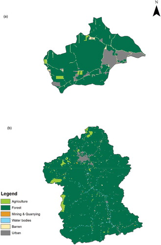
Two unregulated study catchments from SEA, with contrasting characteristics (e.g. area, mean elevation, slope etc.) and non-stationary rainfall–runoff relationships as identified by Saft et al. (2015) and Deb et al. (2019b), were considered in this study. These catchments were Brankeet Creek catchment, Victoria (gauge number 405251; 36.97°S, 145.79°E) and Muttama Creek catchment, New South Wales (NSW) (gauge number 410044; 34.93°S, 148.16°E), hereafter referred as catchments 405251 and 410044, respectively (Fig. 1). Catchment 405251 is narrow and steep (mean slope: 13.6%, which is greater than the 10% mean slope threshold typically used to define a steep catchment; Tani 1997) and comprises of an area of 122 km², whereas 410044 is relatively flat (mean slope: 4.2%, which is less than the 5% mean slope threshold typically used to define a flat catchment; Tani 1997) and has an area of 1061 km². There are four rainfall gauges and one temperature station in each catchment. The annual rainfall is in the ranges 403–1147 mm and 74–1154 mm for catchments 405251 and 410044, respectively, and the mean annual runoff is approx. 121 and 39 mm, respectively. Both catchments comprise of forest cover of greater than 70% of total catchment area (Fig. 2). The soil properties of catchments 405251 and 410044 are provided in the Supplementary material (Fig. S1 and Table S15); the hydrological properties were derived from the Australian soil database (Western and Mckenzie 2004).

Figure 1. Location of the selected study catchments.

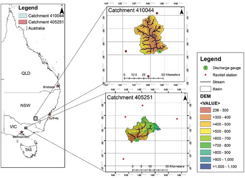
Figure 2. Land-use/land cover map (2012) of catchments (a) 405251 and (b) 410044.

3 Data and methods

3.1 Data

3.1.1 Hydro-meteorological data

The hydro-meteorological data used in this study are given in the Supplementary material (Table S1). Missing values comprise <3% of the entire rainfall data record for both catchments and were assumed to be zero rainfall. Similarly, runoff, maximum and minimum temperature data were missing for <5% of the entire data record. As runoff on a given day simulated by the models is dependent on antecedent catchment conditions, it would be inappropriate to exclude the days with missing runoff when comparing the simulated and observed runoff. This is because excluding the runoff will alter the autocorrelation among the simulated results and this may cascade into a larger difference among the simulated and observed values. Moreover, instead of continuous missing data there were intermittent missing values throughout the dataset which comprised <5% of the whole data record. Also, a comparative study of infilling missing runoff data with different approaches by Gyau-Boakye and Schultz (1994) suggested that infilling missing values when using runoff from previous years for the same day is the best suited method. Therefore, the missing runoff data were infilled by calculating the average runoff on a given day (calculated over the whole data record). A similar approach was also used to infill the missing maximum and minimum temperatures.

3.1.2 Catchment characteristic data

The catchment characteristic data used in this study are given in the Supplementary material (Table S2). The Thiessen polygon approach was used for the calculation of mean areal rainfall in the whole catchment (Brassel and Reif 1979). The potential evapotranspiration (PET) was calculated using the Hargreaves-Samani equation (Hargreaves and Samani 1985). This is because of the finding of Moeletsi et al. (2013), who showed that the Hargreaves-Samani equation performed equally well to the Penman-Monteith equation in semi-arid regions.

Due to the finer spatial resolution of the digital elevation model (DEM), the land-use/land cover and soil maps, they were used directly at their inherent resolution. However, the nearest -neighbour resampling approach (Gonsamo et al. 2011) was employed to enhance the spatial resolution of the leaf area index (LAI) data to the required grid size (900 m).

3.2 Description of rainfall–runoff models

Three structurally different rainfall–runoff models, IHACRES (Jakeman et al. 1990, Croke et al. 2004), HEC-HMS (Scharffenberg 2015) and SWATgrid (Rathjens and Oppelt 2012), were selected to assess the suitability of hydrological models to simulate flow under non-stationarity in rainfall–runoff relationships. The criteria for the selection of these models were based on their applicability, spatial discretization, popularity, cost effectiveness and performances in previous studies.

3.2.1 IHACRES

The IHACRES (v2) model is a continuous, conceptually lumped hydrological model which was developed by the UK Institute of Hydrology and the Australian National University. It is based on the principle of Jakeman et al. (1990), in that the model simulates runoff while considering two modules: a non-linear and a linear module (see Supplementary material, Fig. S2). The non-linear module takes rainfall and temperature/PET as an input and calculates the effective rainfall (U) and catchment moisture flux, while applying the catchment moisture deficit scheme (Croke and Jakeman 2004). The linear module converts the effective rainfall into runoff by generating unit hydrographs for quick and slow flows in the catchment. Further details on the IHACRES model can be found in Croke et al. (2004).

3.2.2 HEC-HMS

The HEC-HMS (v4.2.1) model is a continuous, physically based, semi-distributed hydrological model which uses a Geospatial Hydrologic Modelling Extension (HEC-GeoHMS) to disaggregate the catchment into sub-basins based on the user-defined category of stream networks in the catchment. The model requires a DEM as input and derives the stream networks and elevation properties followed by the subdivision of the catchment. In this study, 30 sub-basins were generated for each of the catchments. The HEC-HMS model includes three main modules: a basin module, a meteorological module and a control specifications module. The physical properties of a catchment, such as the sub-basin area, slope, land use and soil characteristics, are stored in the basin module. The meteorological variables (i.e. rainfall, temperature and PET) of a catchment are stored in the meteorological module. The control specification module stores the user-defined simulation start and end time/date and the computation time step. Further details on the different methods and options are available in Scharffenberg (2015).

In this study, the Soil Conservation Service (SCS) Curve Number (CN) approach was used for calculating excess precipitation. Direct runoff was calculated by the SCS Unit Hydrograph (UH) approach. Also, the constant monthly varying baseflow method was selected for baseflow calculation where the mean monthly baseflow was calculated from the mean monthly runoff by the application of one parameter digital filter method proposed by Lyne and Hollick (1979). The river routing was done by the Muskingum routing model. These approaches have been successfully applied in different catchments ranging from tropical regions (Deb et al. 2018a, Srivastava et al. 2020) to arid catchments (Abushandi and Merkel 2013).

3.2.3 SWATgrid

The SWATgrid model (Rathjens and Oppelt 2012) is a continuous, physically based, fully-distributed hydrological model. The internal structure of the model integrates landscape routing and a grid-based set-up which works along with the Soil and Water Assessment Tool (SWAT) model (Arnold and Allen 1996). The SWATgrid model discretizes a catchment into smaller grids and calculates the runoff components (particularly lateral flow, shallow GW flow and the surface runoff). This is the basic difference in the working principle of the model compared to the traditional SWAT model, which simulates the runoff at a hydrological response unit (HRU) scale. The water balance approach used by the model to calculate the runoff components is as follows:

(1) $S{W}_{t\left(i\right)}=S{W}_o+{\sum }_{i=1}^t\left(R_{day\left(i\right)}-Q_{surf\left(i\right)}-E_{a\left(i\right)}-W_{seep\left(i\right)}-Q_{gw\left(i\right)}\right)$(1)

where SW_t(i) is the soil water content (mm) at time t, SW_o is the initial soil water content (mm), t is the simulation period (days), R_day(i) is the amount of rainfall on the ith day (mm), Q_surf(i) is the surface runoff (mm) on day i, E_a(i) is the amount of PET on day i (mm), W_seep(i) is the amount of water (mm) entering the vadose zone on day i and Q_gw(i) is the amount of baseflow (mm) on day i. The SWATgrid model performs the water balance for each grid and the flow routing through the cells is done by identifying the position of each cell grid. This involves the introduction of a modified topographic index (ranging from 0 to 1) and is calculated based on:

(2) ${\lambda }_i=\mathrm{l}\mathrm{n}\left(\frac{A_i}{\mathrm{t}\mathrm{a}\mathrm{n}\left({\beta }_i\right)\times K_i\times Z_i}\right)\mathrm{\forall }i=1,2,\dots n$(2)

where i is the grid number, λ_i is the topographic index, A_i is the upslope area contributing to per unit contour length (m²), β_i is the slope of the cell (degrees), K_i is the saturated hydraulic conductivity (m d⁻¹) and Z_i is the soil depth (m) for each grid cell. The basic difference in runoff calculation between the SWAT and SWATgrid models is that the latter uses a flow separation index (related to the topographic index) to calculate the spatially distributed proportions of channel and landscape/overland runoff, whereas, in SWAT, a constant flow separation approach is used (Rathjens et al. 2015). In SWATgrid, the SCS-CN method, kinematic storage model and linear tank storage model are used to calculate the surface runoff, lateral runoff and the shallow GW flow respectively from each grid cell. The DEM is used as the basic data to delineate the flow path and defining the grid cells using an external landscape analysis tool called TOPographic PArameteriZation (TOPAZ) toolbox (Garbrecht and Martz 2000). Generally smaller grid sizes (<1000 m) are recommended for flat topography (Beven 1990). Therefore, a grid size of 900 m was used to set up the model at the study catchments, which resulted in 136 and 1180 grids for catchments 405251 and 410044, respectively.

All of these models (i.e. IHACRES, HEC-HMS and SWATgrid) require all four hydro-meteorological datasets as input (as given in Table S1); however, they do not require all catchment characteristics datasets as input. For instance, IHACRES is a simple structured conceptually lumped model and does not require any catchment information other than the catchment size (in km²). On the other hand, the HEC-HMS model requires DEM, land use and land cover and soil map as input. Similarly, the SWATgrid model requires intensive catchment characteristic information including the DEM, land use and land cover, soil map and LAI. It is to be noted that the HEC-HMS requires all the datasets for only one year (data from whichever year is available is sufficient), whereas the SWATgrid model requires temporal data of LAI (since it accounts for the temporal changes in the vegetation cover in runoff simulation).

3.3 Differential split-sample test

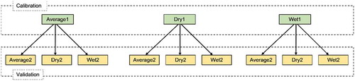
The suitability of the rainfall–runoff models for simulating non-stationary rainfall–runoff relationships was evaluated based on their performance under varying climatic periods. Model calibration and validation was done based on the differential split-sample test (Klemes 1986), in which the hydrological models are calibrated and validated under contrasting climatic conditions. Different periods with varying historical rainfall conditions were chosen based on the recommendations of Li et al. (2012). The steps for identification of different periods at both catchments can be found in Deb et al. (2019a). In total, six time periods of 5 and 9 years were selected for catchments 405251 and 410044, respectively. These periods were termed “Average1”, “Average2”, “Dry1”, “Dry2”, “Wet1” and “Wet2”.

All three hydrological models were calibrated for the Average1, Dry1 and Wet1 periods and validated for the remaining three (i.e. Average2, Dry2 and Wet2 in turn). This resulted in a total of nine calibration and validation sets for each catchment and each of the three models (Fig. 3). The calibration and validation of the models was done for both catchments and was performed using daily observed runoff at the catchment outlets. As per the recommendations of Coron et al. (2012) and Li et al. (2012), the converse calibration/validation (i.e. calibration of models on Average2, Dry2 and Wet2 and validation on Average1, Dry1 and Wet1 periods) was not performed since these steps would lead to unhelpful insights.

Figure 3. Periods during which the hydrological models were calibrated and validated.

3.4 Hydrological model calibration and validation

The number of parameters to be adjusted for model calibration varies within models and the modelling approach selected. For instance, in the case of the IHACRES model, six parameters have to be adjusted. The user inputs the model parameter ranges and the timestep at which the model should apply the grid search approach to find the optimal values for the best objective function (further details are given in Croke et al. 2004). Similarly, for HEC-HMS, six parameters have to be adjusted. The Nelder-Mead approach of auto-calibration (Nelder and Mead 1965) was selected, in which different parameter sets are compared to reach the maximum/minimum of the objective function. In this study, the sum of squared residuals (which emphasizes the water balance) is used as the objective function since it gives more weight to large errors compared to smaller errors (Zhang et al. 2013). Since HEC-HMS is tested for different periods, model parameterization based on the large differences among simulated and observed values is ideal. Also, due to the complicated structure of the SWATgrid model, the number of parameters can range from 10 to 15, or even higher depending on the catchment being studied.

In order to reduce the computation time, a sensitivity test was done for 14 of the main parameters used in the SWATgrid model using the recommended parameter ranges provided in the SWAT user manual for the larger catchment (i.e. 410044) following the approach of Uniyal et al. (2015). The results are given in Table 1. Each of the model parameters was adjusted by ±25% relative to the default value and model simulation was done for each changed parameter. The Nash-Sutcliffe efficiency criterion (NSE) (described in Section 3.5) was calculated based on observed time series and model simulation of the changed model parameters. The NSE was further compared to the NSE obtained based on the observed and default parameter sets. Based on the percent different in NSE, the parameters were grouped into high (>15%), moderate (2–15%) and low (<2%) categories (as per the recommendation of Greets et al. 2009). In this study, we only considered six parameters that were classified as “high” for model calibration (Table 2). The model calibration was done using the ParaSol technique of auto-calibration, which is available in the SWAT-CUP package of the model. Although the sensitivity analysis was done within the recommended range of parameter values, model calibration using parameter values beyond the suggested range may lead to different (possibly better or worse) results and is a limitation of this study which readers should note.

Table 1. Sensitivity analysis of SWATgrid model parameters at catchment 410044.

Parameter	Percent change in NSE (+25% change in parameter)	Percent change in NSE (−25% change in parameter)	Sensitivity level
ALPHA_BF	19.32	18.17	High
Ch_K2	3.26	2.19	Moderate
GWQMN	23.36	27.73	High
SOL_AWC	29.17	21.18	High
SOL_K	17.76	19.17	High
CN2	25.55	26.23	High
ESCO	20.34	19.90	High
CH_N2	1.16	1.92	Low
GW_DELAY	2.33	2.04	Moderate
GW_REVAP	1.77	1.86	Low
RECHARG_DP	1.69	1.96	Low
REVAPMN	7.33	6.94	Moderate
SOL_Z	0.43	0.51	Low
OV_N	0.66	0.72	Low

Table 2. IHACRES, HEC-HMS and SWATgrid model parameter definitions, units and their range used in this study.

Model	Parameter	Definition	Units	Range
IHACRES	τq	Time constant controlling the recession of quickflow	Day	0.5–10
	τs	Time constant controlling the recession of slow flow	Day	10 – 350
	vs	Fraction of slow flow to total flow	(-)	0 – 1
	d	Flow threshold	mm	5 – 550
	e	Temperature to PET conversion factor	(-)	0.01–1.5
	f	Plant stress threshold factor	(-)	0.01–3
HEC-HMS	CN	Curve Number	(-)	1 – 100
	Ip	Percent imperviousness	%	0.5 – 3
	Ia	Initial abstraction	mm	0 – 500
	Lt	Lag time	min	0.1 – 30,000
	K	Muskingum K	hr	0.1–150
	x	Muskingum x	(-)	0 – 0.5
SWATgrid	GWQMN	Threshold depth of water in the shallow aquifer required for return flow to occur	mm	0 – 5000
	SOL_AWC	Available water holding capacity of the soil	mm mm^−1	0 – 1
	ALPHA_BF	Baseflow alpha factor	Day^−1	0 – 1
	SOL_K	Saturated hydraulic conductivity	mm h^−1	0 – 0.15
	CN2	SCS-CN for moisture condition II	(-)	35 – 98
	ESCO	Soil evaporation compensation factor	(-)	0.01 – 1

The grid search for the best parameter set led to 20 000 model iterations for IHACRES model and 10 000 iterations for HEC-HMS. Due to the high computation time for SWATgrid and to avoid over-parameterization, the iterations were limited to 5000. These iterations were done for the model calibration for each of the three periods (i.e. Average1, Dry1 and Wet1) and the parameter sets resulting in the best value of objective function were used for the model validation. The model calibration and validation were done at a daily time step for both catchments.

3.5 Hydrological model performance evaluation

The rainfall–runoff model comparison was done based on the models’ ability to realistically simulate the flow for the model calibration and validation periods (i.e. Average, Dry and Wet). The hydrological model performance assessment was done for the daily flows based on three criteria: Nash-Sutcliffe efficiency (NSE) (Nash and Sutcliffe 1970), root mean square error (RMSE) and percentage bias (PBIAS). The formulae are given in the Supplementary material (Eqs. (S1)–(S3)).

The NSE determines the relative magnitude of residual variance relative to the observed data variance. Its value ranges from – ∞ to 1 and a NSE value of ≥0.65 is considered acceptable (Ritter and Muñoz-Carpena 2013).

The RMSE indicates the magnitude of the errors in simulation by the models (Eq. (S2)). An RMSE value of 0 is ideal; however, for runoff simulation, RMSE values of less than half of the standard deviation of the observed runoff are acceptable (Moriasi et al. 2007).

The PBIAS measures the tendency of the simulated values to be larger or smaller than the observed flows (Eq. (S3)). A negative value indicates the overestimation by the model and vice versa. The optimal value is 0; however, a value within the range ±20% is considered acceptable (Gupta et al. 1999).

Model performance was also assessed based on the comparison of flow–duration curves (FDC) and percent deviation in the percentile flow (10% and 90%) for calibration and validation. As per Tegegne et al. (2017) and Kannan et al. (2018), FDCs can be divided into three classes: high flows (0–10% in FDC; mid-range flows (>10–90% in FDC); and low flows (>90–100% in FDC); they are visually compared to see how close each model simulates flow in each of the three different flow classes.

4 Results

4.1 Identification of Average, Dry and Wet periods

The mean annual rainfall (MAR) varies markedly between the two catchments (Fig. 4(a) and (b)): catchment 405251 receives 967 mm/year, whereas only 571 mm/year is received by catchment 410044. Table 3 shows, for each catchment, the Average, Dry and Wet periods chosen for calibration and validation along with their key statistics. Figure 5 and Table 3 illustrate the range of hydroclimatic conditions that exist in SEA and emphasizes the need for a hydrological model that realistically captures this spatial and temporal non-stationarity.

Table 3. Average, Dry and Wet periods chosen for catchments 405251 and 410044.

Catchment	MAR for whole record (mm)	Periods	Years selected	Percent change in MAR relative to the MAR for the whole record
405251	967	Average1	1976-1980	−3.2
		Dry1	2000-2004	−25.5
		Wet1	1987-1991	15.8
		Average2	1981-1985	0.5
		Dry2	2005-2009	−26.5
		Wet2	1992-1996	15.0
410044	571	Average1	1971-1979	−1.6
		Dry1	1943-1951	−49.9
		Wet1	1962-1970	28.2
		Average2	1980-1988	−2.8
		Dry2	2001-2009	−29.8
		Wet2	1992-2000	22.1

Figure 4. Average1, Average2, Dry1, Dry2, Wet1 and Wet2 periods chosen for model calibration and validation in this study for catchments (a) 405251 and (b) 410044 (MAR represents mean annual rainfall for the whole data record).

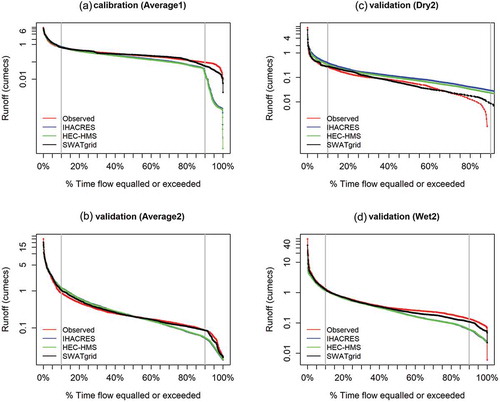
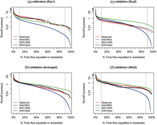
Figure 5. Flow–duration curves for model comparison during (a) calibration (Average1), (b) validation (Average2), (c) validation (Dry2) and (d) validation (Wet2) in case of catchment 405251 (vertical grey lines indicate the division of 10% and 90% flows).

4.2 Model performance at catchment 405251

4.2.1 Calibration: Average1 period

Table 4 shows that the IHACRES model realistically simulates the runoff for the calibration in the Average1 period, with all three model performance statistics within the acceptable range. The calibrated model parameters for the Average1 calibration period are provided in the Supplementary material (Table S3). For validation, the model realistically simulates the runoff for the Average2 period but fails to realistically simulate it for the Dry2 and Wet2 periods. Table 4 also shows similar results for the HEC-HMS model for calibration and validation. In contrast, SWATgrid realistically simulates the runoff for calibration in Average1 and all three cases of model validation (i.e. Average2, Dry2 and Wet2 periods). Notably, the NSE for the SWATgrid model is >0.80 for all cases of calibration and validation. It is also observed that the model overestimates the runoff for validation in Average2 and Dry2 periods (negative values of PBIAS), whereas it underestimates for the Wet2 validation (positive values of PBIAS). Although the IHACRES and HEC-HMS models realistically simulate the runoff for the calibration in the Average1 period, it is evident from Fig. 5(a) (and supplementary Table S9) that both models underestimate low flows. Similarly, the highest and the lower parts of the mid-range flows in the FDC are underestimated by the corresponding models (Fig. 5(b). While considering the Dry2 validation, all three models overestimate the low flows, with high magnitudes for IHACRES and HEC-HMS (Fig. 5(c) and Table S9). Furthermore, for Wet2 validation, both the high and low flows are underestimated by all three models (Fig. 5(d) and Table S9).

Table 4. Model comparison statistics during calibration in Average1 and validation in Average2, Dry2 and Wet2 periods at catchment 405251. Bold figures represent values within an acceptable range as detailed in Section 3.5.

Period	Model	NSE	RMSE (m^3 s^−1)*	PBIAS (%)
Calibration (Average1)	IHACRES	0.83	0.29	10.40
	HEC-HMS	0.80	0.31	18.02
	SWATgrid	0.94	0.17	−2.10
Validation (Average2)	IHACRES	0.76	0.61	−6.40
	HEC-HMS	0.75	0.66	−5.30
	SWATgrid	0.95	0.30	−3.81
Validation (Dry2)	IHACRES	0.47	0.22	−33.45
	HEC-HMS	0.39	0.29	−23.62
	SWATgrid	0.81	0.16	−5.40
Validation (Wet2)	IHACRES	−1.62	1.43	37.44
	HEC-HMS	−1.78	1.45	39.32
	SWATgrid	0.87	0.65	12.74

*acceptable values for RMSE are 0.34, 0.71, 0.17 and 1.02 m³ s⁻¹ for Average1, Average2, Dry2 and Wet2, respectively, and are calculated from the observed runoff for the corresponding periods (as described in Section 3.5).

4.2.2 Calibration: Dry1 period

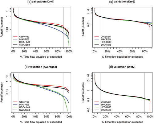
Table 5 shows the model performance statistics obtained from the calibration of the models for the Dry1 period. The calibrated model parameters for the Dry1 calibration period are given in the Supplementary material (Table S4). The results in Table 5 indicate that the IHACRES and SWATgrid models satisfy all three criteria of model evaluation, whereas the calibration of HEC-HMS results in the acceptance of only NSE (≥ 0.65) and PBIAS (≤ ± 20%). For validation of the models for the Average2, Dry2 and Wet2 periods, only SWATgrid is noted to simulate the runoff realistically (i.e. all three criteria are met satisfactorily). The NSE and RMSE obtained for the model validation for the Dry2 period indicate that the IHACRES and HEC-HMS models fail to simulate the runoff realistically. Although the NSE and PBIAS obtained for the respective models for the Wet2 validation are within acceptable ranges, the RMSE shows higher values (1.04 and 1.11 m³ s⁻¹, respectively) compared to the acceptable value of 1.02 m³ s⁻¹.

Table 5. Model comparison statistics during calibration in Dry1 and validation in Average2, Dry2 and Wet2 periods at catchment 405251. Bold figures represent values within an acceptable range as detailed in Section 3.5.

Period	Model	NSE	RMSE (m^3 s^−1)*	PBIAS (%)
Calibration (Dry1)	IHACRES	0.73	0.32	7.50
	HEC-HMS	0.71	0.46	13.72
	SWATgrid	0.92	0.15	3.61
Validation (Average2)	IHACRES	0.68	1.02	−14.62
	HEC-HMS	−6.12	1.44	97.52
	SWATgrid	0.84	0.43	1.48
Validation (Dry2)	IHACRES	0.49	0.21	−3.29
	HEC-HMS	0.51	0.29	−6.86
	SWATgrid	0.87	0.16	3.59
Validation (Wet2)	IHACRES	0.70	1.04	5.10
	HEC-HMS	0.67	1.11	5.33
	SWATgrid	0.78	0.44	3.66

*Acceptable values for RMSE are 0.32, 0.71, 0.17 and 1.02 m³ s⁻¹ for Dry1, Average2, Dry2 and Wet2, respectively, and are calculated from the observed runoff for the corresponding periods (as described in Section 3.5).

The FDCs show that all three models significantly underestimate the low flows for the Dry1 calibration and Average2 validation periods (Fig. 6(a) and (b), Table S10). Although SWATgrid also shows a slight underestimation for the corresponding periods, it follows the same pattern as the observed runoff. All three models overestimate the low flows for the Dry2 validation with maximum deviation observed for the IHACRES followed by the HEC-HMS model (Fig. 6(c), Table S10). Similarly, all three models overestimate the low flows for the Wet2 validation (Fig. 6(d)). In summary, among all three models, SWATgrid simulated the flow within the acceptable range of accuracy for the Dry1 calibration and all three cases of validation.

Figure 6. Flow–duration curves for model comparison during (a) calibration (Dry1), (b) validation (Average2), (c) validation (Dry2) and (d) validation (Wet2) in case of catchment 405251 (vertical grey lines indicate the division of 10% and 90% flows).

4.2.3 Calibration: Wet1 period

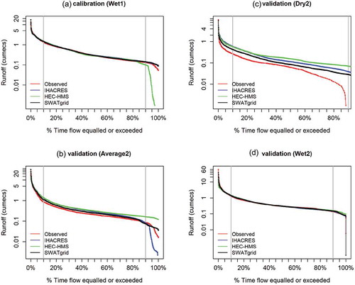
Table 6 shows the results of the model calibration for the Wet1 period at catchment 405251. The calibrated model parameters for the Wet1 calibration period are given in Table S6. The results in Table 6 indicate that all three models can realistically simulate the runoff in the calibration and Wet2 validation periods. Table 6 also shows that IHACRES and SWATgrid models overestimate the runoff for the Wet1 calibration (negative PBIAS), whereas the models underestimate it for Wet2 validation (positive PBIAS). In addition, the IHACRES and HEC-HMS models give NSE values of 0.75 and 0.71, respectively, for the Average2 validation period, while the RMSE and PBIAS reveal poor simulation by the models for the corresponding period. Very poor model performance is observed for all three models in the Dry2 validation period, although the best performance is noted for the SWATgrid model. The NSE for SWATgrid varies from 0.57 to 0.95 for Dry2 validation and Wet1 calibration, respectively. These NSE values for the models reflect that the best model performance is obtained for the Wet period, whereas the model performs poorly in the low flow period.

Table 6. Model comparison statistics during calibration in Wet1 and validation in Average2, Dry2 and Wet2 periods at catchment 405251. Bold figures represent values within an acceptable range as detailed in Section 3.5.

Period	Model	NSE	RMSE (m^3 s^−1)*	PBIAS (%)
Calibration (Wet1)	IHACRES	0.78	0.46	−0.28
	HEC-HMS	0.77	0.47	2.41
	SWATgrid	0.95	0.21	−1.42
Validation (Average2)	IHACRES	0.75	0.63	−17.82
	HEC-HMS	0.71	0.62	−20.90
	SWATgrid	0.86	0.34	−14.43
VALIDATION (Dry2)	IHACRES	0.41	0.49	−51.15
	HEC-HMS	0.33	0.58	−54.20
	SWATgrid	0.57	0.27	−28.85
Validation (Wet2)	IHACRES	0.66	0.85	15.26
	HEC-HMS	0.71	0.96	16.21
	SWATgrid	0.87	0.59	3.39

*acceptable values for RMSE are 0.47, 0.71, 0.17 and 1.02 m³ s⁻¹ for Wet1, Average2, Dry2 and Wet2, respectively, and are calculated from the observed runoff for the corresponding periods (as described in Section 3.5).

The FDCs for the Wet1 calibration and Wet2 validation show that all three models can simulate runoff in a similar pattern to the observed runoff. The only deviation is noted for the low flows in the case of calibration and validation with HEC-HMS and SWATgrid, respectively (Fig. 7(a) and (d)). The FDC for the validation of the Average2 period indicates that HEC-HMS overestimates and IHACRES and SWATgrid underestimate the low (90th percentile) flows (Fig. 7(b), Table S11). Furthermore, the FDC for the Dry2 validation indicates that all three models overestimate the low flows by a large margin (Fig. 7(c), Table S11). This is also supported by the PBIAS statistics, where high negative values are noted (mentioned above). These results illustrate that among all three models the SWATgrid model simulates the runoff with the highest accuracy; however, it is limited to the validation in the Average2 and Wet2 periods in the catchment.

Figure 7. Flow–duration curves for model comparison during (a) calibration (Wet1), (b) validation (Average2), (c) validation (Dry2) and (d) validation (Wet2) in case of catchment 405251 (vertical grey lines indicate the division of 10% and 90% flows).

4.3 Model performance at catchment 410044

4.3.1 Calibration: Average1 period

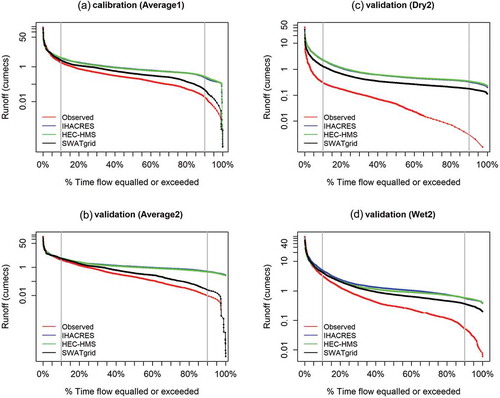
Table 7 shows the result for model calibration for the Average1 period at catchment 410044. The calibrated model parameters for the Average1 calibration period are given in Table S6. The results in Table 7 indicate that the NSE is negative in all the cases of IHACRES and HEC-HMS model calibration and validation. Also, the higher magnitudes of RMSE relative to the threshold value further confirm the inability of both models to realistically simulate the runoff in the Average1 calibration and validation for the remaining three periods (i.e. Average2, Dry2 and Wet2). Furthermore, it is evident from Table 7 that all of the three models overestimate the runoff irrespective of the periods considered (negative PBIAS). Although the SWATgrid model is able to simulate the runoff within an acceptable range of NSE, RMSE and PBIAS, this is only for the Average1 calibration and Average2 validation. The higher value of PBIAS > ±20% for the Wet2 validation of SWATgrid model refers to the inability of the model to realistically simulate the runoff.

Table 7. Model comparison statistics during calibration in Average1 and validation in Average2, Dry2 and Wet2 periods at catchment 410044. Bold figures represent values within an acceptable range as detailed in Section 3.5.

Period	Model	NSE	RMSE (m^3 s^−1)*	PBIAS (%)
Calibration (Average1)	IHACRES	−0.28	4.74	−24.72
	HEC-HMS	−0.53	4.38	−31.15
	SWATgrid	0.85	1.09	−11.82
Validation (Average2)	IHACRES	−0.38	4.39	−29.82
	HEC-HMS	−0.44	5.20	−26.82
	SWATgrid	0.90	0.89	−9.20
Validation (Dry2)	IHACRES	−0.16	2.14	−82.09
	HEC-HMS	−0.19	2.06	−56.21
	SWATgrid	0.43	0.97	−69.81
Validation (Wet2)	IHACRES	−0.06	3.78	−34.95
	HEC-HMS	−0.28	2.85	−26.69
	SWATgrid	0.67	1.89	−21.89

*acceptable values for RMSE are 3.12, 2.84, 0.52 and 2.34 m³ s⁻¹ for Average1, Average2, Dry2 and Wet2, respectively, and are calculated from the observed runoff for the corresponding periods (as described in Section 3.5).

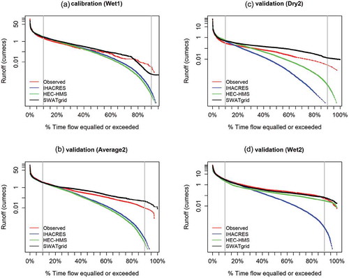
These results are further supported by the FDCs generated from the observed and simulated runoffs by the models. It can be clearly seen that all three models overestimate the low flows during all cases of calibration and validation (Fig. 8, Table S12). Also, for Average2 model validation, the IHACRES and HEC-HMS models overestimate the mid-range and low flows. Although SWATgrid also shows a slight overestimation for the mid-range flow, yet it can realistically simulate the low flows (Fig. 8(b)). Furthermore, all three models overestimate the mid-range and low flows during the Dry2 and Wet2 validation with higher magnitudes of variation in the Dry2 case (Fig. 8(c) and (d), Table S12). In brief, only the SWATgrid model can realistically simulate the runoff; however, it is limited to the model calibration and validation during the Average periods.

Figure 8. Flow–duration curves for model comparison during (a) calibration (Average1), (b) validation (Average2), (c) validation (Dry2) and (d) validation (Wet2) in case of catchment 410044 (vertical grey lines indicate the division of 10% and 90% flows).

4.3.2 Calibration: Dry1 period

Table 8 highlights the results of model calibration for the Dry1 period at catchment 410044. The calibrated model parameters for the Dry1 calibration period are given in Table S7. The results in Table 8 suggest that both the IHACRES and HEC-HMS models simulate the runoff unrealistically, with negative NSE values. The negative NSE values indicate that the mean observed value is a better predictor compared to the simulated values (Moriasi et al. 2007) and, therefore, the model results are unacceptable. Although acceptable NSE and RMSE are observed for the SWATgrid model, PBIAS reflects unrealistic model performance (30.31%). The results for the model validation suggest that only SWATgrid can realistically simulate the runoff for the Average2 and Dry2 validation periods (all three criteria are met).

Table 8. Model comparison statistics during calibration in Dry1 and validation in Average2, Dry2 and Wet2 periods at catchment 410044. Bold figures represent values within an acceptable range as detailed in Section 3.5.

Period	Model	NSE	RMSE (m^3 s^−1)*	PBIAS (%)
Calibration (Dry1)	IHACRES	−17.42	2.22	210.41
	HEC-HMS	−14.42	2.36	200.41
	SWATgrid	0.81	0.71	−30.31
Validation (Average2)	IHACRES	−8.84	5.06	22.71
	HEC-HMS	−8.51	4.12	−31.10
	SWATgrid	0.84	1.66	18.82
Validation (Dry2)	IHACRES	−0.05	4.15	62.88
	HEC-HMS	−1.13	1.58	−66.25
	SWATgrid	0.87	0.29	−16.72
Validation (Wet2)	IHACRES	−6.90	3.86	113.46
	HEC-HMS	−4.74	2.89	−24.51
	SWATgrid	0.39	2.45	99.12

*acceptable values for RMSE are 1.08, 2.84, 0.52 and 2.34 m³ s⁻¹ for Dry1, Average2, Dry2 and Wet2, respectively, and are calculated from the observed runoff for the corresponding periods (as described in Section 3.5).

The FDCs indicate that the IHACRES model underestimates the mid-range and low flows in all cases of model calibration and validation (Fig. 9, Table S13). A relatively better performance is observed for the HEC-HMS, where the model overestimates the runoff only for the validation (Average2, Dry2 and Wet2) periods (Fig. 9(b), (c) and (d), Table S13). Indeed, the best performance is observed for the SWATgrid model; however, a small bump in the simulated flows can be seen in the mid-range flows in case of Dry1 calibration (overestimation) (Fig. 9(a)) and the Wet2 validation (underestimation) (Fig. 9(b)). This may be the possible cause for the observed over- and underestimation of the runoff (reflected by PBIAS) for the Dry1 calibration and Wet2 validation, respectively.

Figure 9. Flow–duration curves for model comparison during (a) calibration (Dry1), (b) validation (Average2), (c) validation (Dry2) and (d) validation (Wet2) in case of catchment 410044 (vertical grey lines indicate the division of 10% and 90% flows).

4.3.3 Calibration: Wet1 period

The calibrated model parameters for the Wet1 calibration period are given in Table S8. Similar to the previous results, the IHACRES and HEC-HMS models produce a negative NSE value for Wet1 calibration and validation for all three periods (Table 9). In addition, RMSE values are also noted to be higher than the threshold values for both calibration and validation. Additionally, PBIAS indicates that both models underestimate the runoff during the Wet1 calibration and validation for Average2 and Dry2 periods (Table 9). For the Wet2 validation, IHACRES is noted to underestimate the runoff and HEC-HMS is observed to be in close proximity of the observed runoff (PBIAS = 7.01%). However, the SWATgrid model simulates the runoff in good agreement for the Wet1 calibration and validation for Average2 and Wet2 periods, but fails to realistically simulate the runoff for the Dry2 validation period.

Table 9. Model comparison statistics during calibration in Wet1 and validation in Average2, Dry2 and Wet2 periods at catchment 410044. Bold figures represent values within an acceptable range as detailed in Section 3.5.

Period	Model	NSE	RMSE (m^3 s^−1)*	PBIAS (%)
Calibration (Wet1)	IHACRES	−0.11	3.55	21.60
	HEC-HMS	−0.08	3.54	30.30
	SWATgrid	0.83	1.69	6.30
Validation (Average2)	IHACRES	−0.76	3.95	37.91
	HEC-HMS	−0.95	4.18	40.21
	SWATgrid	0.91	1.18	−3.53
Validation (Dry2)	IHACRES	−0.81	1.06	23.62
	HEC-HMS	−0.67	1.12	20.31
	SWATgrid	0.49	0.81	−32.41
Validation (Wet2)	IHACRES	−0.09	3.09	38.31
	HEC-HMS	−0.06	3.34	7.01
	SWATgrid	0.88	1.36	16.12

*acceptable values for RMSE are 2.62, 2.84, 0.52 and 2.34 m³ s⁻¹ for Wet1, Average2, Dry2 and Wet2, respectively, and are calculated from the observed runoff for the corresponding periods (as described in Section 3.5).

The FDCs further support the outcomes of the model performance evaluation, while indicating the underestimation of the mid-range and low flows in case of the IHACRES and HEC-HMS models for calibration and validation (Fig. 10, Table S14). Additionally, the curves also show that the SWATgrid model overestimates the mid-range and low flows for the Dry2 validation (Fig. 10(c)), whereas it simulates the runoff in good agreement for the remaining three periods. The FDCs also show that all the models can simulate high flows in good agreement with the observed flow and, therefore, the major concern is the inability of the models to realistically simulate low flows, especially for the Dry periods.

Figure 10. Flow–duration curves for model comparison during (a) calibration (Wet1), (b) validation (Average2), (c) validation (Dry2) and (d) validation (Wet2) in case of catchment 410044 (vertical grey lines indicate the division of 10% and 90% flows).

5 Discussion

The results for the smaller catchment (405251) show that when the models are calibrated on the Average1 and Dry1 periods, only the fully distributed (SWATgrid) model can simulate the runoff realistically under non-stationarity (i.e. for the Average2, Dry2 and Wet2 validation periods). The simplicity of the model structure and not accounting for shallow GW flow in the IHACRES and HEC-HMS models is a likely cause for their unrealistic simulations. Although the HEC-HMS model considers constant monthly baseflow, it does not display the cessation of the SW–GW interaction, which is an important phenomenon in arid and semi-arid regions during multi-year droughts (Kiem and Verdon-Kidd 2009, 2010, Vaze et al. 2010, Saft et al. 2015, Deb et al. 2019a, 2019b). Additionally, the river routing (Muskingum routing model) is likely to be poorly represented by the HEC-HMS model in this catchment as the approach performs poorly in smaller catchments (Pandey et al. 2018). Despite the fact that SWATgrid also lacks detailed GW modelling (which involves the shallow GW and riverbed interaction), it still calculates the lateral and shallow GW flow through kinematic wave approximation and linear tank storage model, respectively, within each grid cell (Sloan and Moore 1984). Also, the superior performance of the SWATgrid model for Wet2 validation could be due to the principle of spatial disaggregation of inputs in the model. This allows the model to calculate the flow from the ephemeral streams (since the catchment is steep), possibly generated during the Wet2 validation periods (Ghosh et al. 2016) – such processes are not captured by the IHACRES and HEC-HMS models.

The poor performance of the SWATgrid model for Dry2 validation on Wet1 calibration can be attributed to the static nature of the flow separation index (linked to the topographic index). Since the saturation of a watershed is of dynamic nature (Deb et al. 2018b), the model fails to estimate the precise soil moisture content of the vadose zone and ultimately the runoff (Vereecken et al. 2008). Another possible explanation may be the use of the poor resolution of LAI. The accuracy of the temporal changes in vegetation cover could be reduced in the resampling approach for the Dry2 period, which affects the interception (which is a major component of flow generation in the semi-arid regions). Since, tree die-off is a common phenomenon during multi-year droughts (Saft et al. 2015), this results in more barren land and, therefore, a larger amount of rain water is lost through percolation and PET instead of runoff generation (Pilgrim et al. 1988). Considering this and the possible error in LAI, a larger area with vegetation cover is used in the simulation. This possibly aggregates to more lateral flow during simulation since vegetation leads to higher water retention in the soil root zone (which contributes to lateral flow) (Kim and Mohanty 2016).

For the larger catchment (i.e. 410044), only the SWATgrid model performs reasonably well by realistically simulating runoff, generally in two cases during validation when calibrated for each Average1, Dry1 and Wet1 conditions. The probable cause for the poor performance of the IHACRES and HEC-HMS models in the Dry2 validation period is due to their inability in consideration of the temporal changes in the vegetation cover, such as tree die-off, is common during multi-year droughts (Saft et al. 2015, Deb et al. 2019b). Also, the runoff generation in a catchment is highly sensitive to the spatial variability of antecedent soil moisture (Li et al. 2012). During Dry2 periods the soil moisture is more heterogeneous relative to the Wet2 periods (Minet et al. 2011) and, since the lumped and semi-distributed model structures avoid the consideration of the spatial variability of soil moisture, these models are likely to simulate an erroneous runoff. Furthermore, the unavailability of sufficient high flows during droughts to adequately calibrate the model parameters can also be another major factor for the unrealistic simulations by the models in Wet2 validation on Dry1 calibration (Gan et al. 1997). This suggests that the simulations by IHACRES and HEC-HMS models are unrealistic for similar reasons whereas different factors (e.g. inappropriate grid size selection) are responsible for the unrealistic simulations of SWATgrid in the larger catchment.

Coarse grid size in SWATgrid contributes to reducing the mean slope and increasing the slope length (Wu et al. 2008, Buakhao and Kangrang 2016). This further increases the topographic index of the SWATgrid model, which translates into higher channelized flow in the catchment (Kumar et al. 2017). Pignotti et al. (2017) showed that the mean slope in a catchment changes from 21 to 0.5% for the consideration of grid sizes of 90 and 1000 m, respectively, while modelling in SWATgrid. Although several studies have suggested a different optimal grid size, a general size of <1000 m is employed. The finer grid size requires more computation time. For instance, in this study, in the automatic calibration of the SWATgrid model on 5 years with 5000 iterations for a single period (e.g. Average1), the model required approximately 125 h of processing time (Intel Xeon® CPU E5-2623 v3 @3.00 GHz, 64 GB RAM processor). This is computationally very tedious when compared to 50 min (20 000 iterations) and 8.5 h (10 000 iterations) for IHACRES and HEC-HMS models, respectively, for the same calibration duration (i.e. 5 years). Therefore, in order to minimize the computational time, a 900-m grid size was chosen. This is possibly too coarse and, therefore, the model may have overestimated the mid-range and low flows for the Dry2 and Wet2 periods. Nevertheless, the performance of the distributed model (SWATgrid) weakens in the larger catchment compared to the smaller catchment.

Another major cause of the poor performance of all three models in the larger catchment possibly underlies in the governing principle of the models. IHACRES calculates runoff in a simplistic way by routing the rainfall excess into “quickflow” and “slowflow”. This does not take into account the physical complexities of larger catchments relative to smaller ones. Additionally, the unit hydrograph theory employed by the model for developing transfer function in hydrograph separation does not always agree with the physical reality of large catchments due to the inherent spatial heterogeneity (Bonell 1993). HEC-HMS and SWATgrid generate runoff on the principle of infiltration excess and in semi-arid headwater area (predominant in larger catchments), and saturation excess overland flow dominates the runoff (Ries et al. 2017). This saturation excess flow is most likely to be true given that Australian catchments have a hard salt crust in the shallow soil (Szabolcs 1991, Shimojima et al. 2013) contributing to quick saturation of the topsoil. Since high-intensity rainfall is unusual in the larger catchment (semi-arid region), a relatively lower runoff is generated, whereas, due to shallow soil with lower water holding capacity (see Table S15), both models simulate higher runoff and perform poorly. This suggests that further investigation is needed into the model evaluation for different catchment sizes, particularly the use of saturation excess models, such as REWASH (Zhang and Savenije 2005) and HGSS (Willgoose and Perera 2001).

Overall, SWATgrid showed the best performance among all three models at both catchments. This can be attributed to the time variant model parameters, particularly CN2, ALPHA_BF, ESCO and SOL_AWC (Table 1), which are adjusted at a daily time scale based on the soil moisture conditions, land-use pattern, etc. in the model calibration and validation periods (Uniyal et al. 2015). In contrast, all the model parameters are time invariant over a simulation period in both IHACRES and HEC-HMS, except for the CN parameter in the case of HEC-HMS. Therefore, under different climatic periods (i.e. under rainfall–runoff non-stationarity), the SWATgrid model tailors its parameters and results in an improved performance. The better suitability of distributed models under hydroclimatic variability resulting from time-varying model parameters are also reported by Zhang et al. (2015) and Ahmadi et al. (2019), who applied models under diverse hydroclimatic conditions in semi-arid regions.

The findings of this study are widely applicable for water management studies under climate change. A rainfall–runoff model is generally applied based on the traditional approach of calibration and validation under similar climatic conditions. However, while considering climate change, this may not be true, since severe droughts are projected to be more frequent in the arid and semi-arid regions (Soh et al. 2008, Sarr 2012, Misra 2014). Therefore, the stationarity of the rainfall–runoff relationship is questionable. In such cases, the differential split-sample test serves as a suitable strategy for pre-application model assessment, in which the models should be tested for at least three periods with different climatic conditions (e.g. Average, Dry, Wet) to understand potential errors in hydrological simulations due to non-stationarity in rainfall–runoff relationships.

For SEA and other arid and semi-arid regions, catchment characteristics and other influences on the rainfall–runoff relationship change during multi-year droughts (van Dijk et al. 2013, Van Loon 2015, Van Loon et al. 2016, Kiem et al. 2016). Conceptually lumped models and other models that do not realistically account for the processes that contribute to this non-stationarity in rainfall–runoff relationships will continue to underperform in catchments that experience large hydroclimatic variability and multi-year/decadal droughts. One may argue that semi- or fully-distributed models are more suitable since they are physically based and are spatially explicit. However, this study reveals that they also fail in the accurate representation of runoff under non-stationary conditions, especially in large and flat catchments. The findings in this paper and in other studies (e.g. Vaze et al. 2010, Chiew et al. 2014, Saft et al. 2015, Deb et al. 2019a, 2019b) suggest that what is missing in the hydrological model structures is a realistic parameterization of SW–GW interactions that occur in arid and semi-arid catchments and, most importantly, how these interactions vary in space and time. This finding corresponds to two of the 23 unsolved problems in hydrology – numbers 6 and 19 – identified by the broad hydrological community (Blöschl et al. 2019). Therefore, further investigation on the development and testing of a revised version of SWATgrid with dynamic flow separation index and the inclusion of the detailed GW flow modelling is essential. Otherwise, another potential solution is a coupled SWATgrid and GW model (e.g. MODFLOW).

6 Conclusion

This study compares how three rainfall–runoff models – conceptually lumped (IHACRES), physically based, semi-distributed (HEC-HMS) and fully-distributed (SWATgrid) – simulate runoff under non-stationary hydroclimatic conditions for two different catchments in SEA. The results show that only the SWATgrid model can realistically simulate runoff in the smaller catchment under most hydroclimatic conditions, though it fails when the model is calibrated in Dry conditions and validated in Wet. Similarly, SWATgrid also performs reasonably well in comparison to IHACRES and HEC-HMS, although it fails for one climatic period (during validation for calibration at each climatic period).

While the traditional approach in the application of rainfall–runoff models assumes climate stationarity, this appears to be invalid in areas such as SEA because (a) hydrological processes change during multi-year droughts and (b) these changes translate into erroneous rainfall–runoff model simulations. It is also emphasized that a differential split-sample test with at least three periods representative of average, dry and wet hydroclimatic conditions should become the standard for pre-application model assessment and selection.

The results also highlight that the topographic index applied in the SWATgrid model is not always successful in realistically simulating runoff, especially in flat basins. In addition, SW–GW interaction is a major influence on the non-stationarity of rainfall–runoff relationships, especially in arid and semi-arid catchments with high spatial and temporal hydroclimatic variability and further research is needed to capture this in rainfall–runoff modelling.

These findings highlight the importance of testing the existing rainfall–runoff models rigorously in different climatic conditions prior to their application in the planning of water management and climate adaptation strategies. Further research is recommended that involves coupling fully-distributed rainfall–runoff models with GW flow models to enable more realistic runoff simulations in arid and semi-arid catchments where non-stationarity in the rainfall–runoff relationships exists. These insights are in line with and contribute to, the aims and priorities of the International Association of Hydrological Sciences decade (2013–2022) Panta Rhei (Montanari et al. 2013).

Acknowledgements

Thanks are given to Dr Alison Oke (Bureau of Meteorology, VIC, Australia) and Dr Stefan Kern (ICDC, University of Hamburg) for providing information about the online data repositories and the LAI dataset for the Australian continent respectively. Thanks also to Mr Matthew Armstrong (University of Newcastle) for his constructive criticism on earlier versions of this paper and to Mr Olivier Rey-Lescure (University of Newcastle) for providing elevation data and catchment boundary information.

Disclosure statement

The authors declare that there is no conflict of interest associated with this paper.

Supplementary material

Supplemental data for this article can be accessed here.

Additional information

Funding

Proloy Deb is funded by a University of Newcastle International Postgraduate Research Scholarship (UNIPRS) and a University of Newcastle Postgraduate Research Scholarship Central (UNRSC 50:50). Funding for this research was also provided by Australian Research Council Linkage [Grant LP120200494], with further funding and/or in-kind support also provided by the NSW Office of Environment and Heritage, Sydney Catchment Authority, Hunter Water Corporation, NSW Office of Water and NSW Department of Finance and Services.

References

- Abushandi, E.H. and Merkel, B.J., 2013. Modelling rainfall runoff relations using HEC-HMS and IHACRES for a single rain event in an arid region of Jordan. Water Resource Management, 27 (7), 2391–2409. doi:10.1007/s11269-013-0293-4
- Ahmadi, M., et al., 2019. Comparison of the performance of SWAT, IHACRES and artificial neural networks models in rainfall–runoff simulation (case study: Kan watershed, Iran). Physics and Chemistry of the Earth. doi:10.1016/j.pce.2019.05.002
- Ahooghalandari, M., Khiadani, M., and Kothapalli, G., 2015. Assessment of artificial neural networks and IHACRES models for simulating streamflow in Marillana catchment in the Pilbara, Western Australia. Australian Journal of Water Resources, 19 (2), 116–126. doi:10.1080/13241583.2015.1116183
- Ajami, H., et al., 2017. On the non-stationarity of hydrological response in anthropogenically unaffected catchments: an Australian perspective. Hydrology and Earth System Sciences, 21 (1), 281–294. doi:10.5194/hess-21-281-2017
- Al-Qurashi, A., et al., 2008. Application of the Kineros2 rainfall–runoff model to an arid catchment in Oman. Journal of Hydrology, 355, 91–105. doi:10.1016/j.jhydrol.2008.03.022
- Ao, T., et al., 2006. Relating BTOPMC model parameters to physical features of MOPEX basins. Journal of Hydrology, 320 (1–2), 84–102. doi:10.1016/j.jhydrol.2005.07.006
- Arnold, J.G. and Allen, P.M., 1996. Estimating hydrologic budgets for three Illinois watersheds. Journal of Hydrology, 176 (1–4), 57–77. doi:10.1016/0022-1694(95)02782-3
- Benke, K.K., Lowell, K.E., and Hamilton, A.J., 2008. Parameter uncertainty, sensitivity analysis and prediction error in a water-balance hydrological model. Mathematical and Computer Modelling, 47, 1134–1149. doi:10.1016/j.mcm.2007.05.017
- Beven, K., 1990. Changing ideas in hydrology — the case of physically based models — comment. Journal of Hydrology, 120 (1–4), 405–407. doi:10.1016/0022-1694(90)90161-P
- Beven, K., 2007. Towards integrated environmental models of everywhere: uncertainty, data and modelling as a learning process. Hydrological and Earth System Sciences, 11 (1), 460–467. doi:10.5194/hess-11-460-2007
- Beven, K., 2012. Rainfall–runoff Modelling. The Primer. 2nd ed. Chichester, UK: John Wiley & Sons. doi:10.1002/9781119951001
- Beven, K., 2013. So how much of your error is epistemic? Lessons from Japan and Italy. Hydrological Processes, 27 (11), 1677–1680. doi:10.1002/hyp.9648
- Blöschl, G., et al., 2019. Twenty-three unsolved problems in hydrology (UPH) – a community perspective. Hydrological Sciences Journal, 64, 1141–1158. doi:10.1080/02626667.2019.1620507
- Bonell, M., 1993. Progress in the understanding of runoff generation dynamics in forests. Journal of Hydrology, 150 (2–4), 215–275. doi:10.1016/0022-1694(93)90112-M
- Boughton, W., 2005. Catchment water balance modelling in Australia 1960-2004. Agricultural Water Management, 71 (2), 91–116. doi:10.1016/j.agwat.2004.10.012
- Brassel, K.E. and Reif, D., 1979. A procedure to generate Thiessen polygons. Geographical Analysis, 11 (3), 289–303. doi:10.1111/j.1538-4632.1979.tb00695.x
- Buakhao, W. and Kangrang, A., 2016. DEM resolution impact on the estimation of the physical characteristics of watersheds by using SWAT. Advances in Civil Engineering, 2016, 1–9. doi:10.1155/2016/8180158
- Chiew, F.H.S., 2006. Estimation of rainfall elasticity of streamflow in Australia. Hydrological Sciences Journal, 51 (4), 613–625. doi:10.1623/hysj.51.4.613
- Chiew, F.H.S., et al., 2014. Observed hydrologic non-stationarity in far south-eastern Australia: implications for modelling and prediction. Stochastic Environmental Research and Risk Assessment, 28 (1), 3–15. doi:10.1007/s00477-013-0755-5
- Coron, L., et al., 2012. Crash testing hydrological models in contrasted climate conditions: an experiment on 216 Australian catchments. Water Resources Research, 48 (5), W05552. doi:10.1029/2011WR011721
- Croke, B.F.W. and Jakeman, A.J., 2004. A catchment moisture deficit module for the IHACRES rainfall–runoff model. Environmental Modelling & Software, 19 (1), 1–5. doi:10.1016/j.envsoft.2003.09.001
- Croke, B.F.W., Merritt, W.S., and Jakeman, A.J., 2004. A dynamic model for predicting hydrologic response to land cover changes in gauged and ungauged catchments. Journal of Hydrology, 291 (1–2), 115–131. doi:10.1016/j.jhydrol.2003.12.012
- Deb, P., et al., 2018b. Variability of soil physicochemical properties at different agroecological zones oh Himalayan region: Sikkim, India. Environment, Development and Sustainability. doi:10.1007/s10668-018-0137-8
- Deb, P., Babel, M.S., and Denis, A.F., 2018a. Multi-GCMs approach for assessing climate change impact on water resources in Thailand. Modeling Earth Systems and Environment, 4 (2), 825–839. doi:10.1007/s40808-018-0428-y
- Deb, P., Kiem, A.S., and Willgoose, G., 2019a. A linked surface water-groundwater modelling approach to more realistically simulate rainfall–runoff non-stationarity in semi-arid regions. Journal of Hydrology, 575, 273–291. doi:10.1016/j.jhydrol.2019.05.039
- Deb, P., Kiem, A.S., and Willgoose, G., 2019b. Mechanisms influencing non-stationarity in rainfall–runoff relationships in southeast Australia. Journal of Hydrology, 571, 749–764. doi:10.1016/j.jhydrol.2019.02.025
- Dwarakish, G.S. and Ganasri, B.P., 2015. Impact of land use change on hydrological systems: A review of current modeling approaches. Cogent Geoscience, 1 (1), 1115691. doi:10.1080/23312041.2015.1115691
- Fowler, K.J.A., et al., 2016. Simulating runoff under changing climatic conditions: revisiting an apparent deficiency of conceptual rainfall–runoff models. Water Resources Research, 52, 1820–1846. doi:10.1002/2015WR018068
- Gallant, A.J.E., et al., 2012. Understanding hydroclimate processes in the Murray-Darling Basin for natural resources management. Hydrology and Earth System Science, 16 (7), 2049–2068. doi:10.5194/hess-16-2049-2012
- Gan, T.Y., Dlamini, E.M., and Biftu, G.F., 1997. Effects of model complexity and structure, data quality, and objective functions on hydrologic modeling. Journal of Hydrology, 192 (1–4), 81–103. doi:10.1016/S0022-1694(96)03114-9
- Gao, C., et al., 2016. Hydrological model comparison and assessment: criteria from catchment scales and temporal resolution. Hydrological Science Journal, 61 (10), 1941–1951. doi:10.1080/02626667.2015.1057141
- Garbrecht, J. and Martz, L.W., 2000. Topaz user manual: version3.1. Technical Report. Oklahoma.
- Gelfan, A., et al., 2015. Testing the robustness of the physically-based ECOMAG model with respect to changing conditions. Hydrological Sciences Journal, 60 (7–8), 1266–1285. doi:10.1080/02626667.2014.935780
- Ghosh, D.K., Wang, D., and Zhu, T., 2016. On the transition of base flow recession from early stage to late stage. Advances in Water Resources, 88, 8–13. doi:10.1016/J.ADVWATRES.2015.11.015
- Gonsamo, A., Pellikka, P., and King, D.J., 2011. Large-scale leaf area index inversion algorithms from high-resolution airborne imagery. International Journal of Remote Sensing, 32 (14), 3897–3916. doi:10.1080/01431161003801302
- Greets, S., et al., 2009. Simulating yield response of quinoa to water availability with AquaCrop. Agronomy Journal, 101, 498–508.
- Gudmundsson, L., Greve, P., and Seneviratne, S.I., 2016. The sensitivity of water availability to changes in the aridity index and other factors—A probabilistic analysis in the Budyko space. Geophysical Research Letters, 43 (13), 6985–6994. doi:10.1002/2016GL069763
- Gupta, H.V., Sorooshian, S., and Yapo, P.O., 1999. Status of automatic calibration for hydrologic models: comparison with multilevel expert calibration. Journal of Hydrologic Engineering, 4 (2), 135–143. doi:10.1061/(ASCE)1084-0699(1999)4:2(135)
- Gyau-Boakye, P., and Schultz, G.A., 1994. Filling gaps in runoff time series in west africa. Hydrological Sciences Journal, 39 (6), 621–636. doi:10.1080/02626669409492784
- Hargreaves, G.H. and Samani, Z.A., 1985. Reference crop evapotranspiration from ambient air temperature. American Society Agricultural and Biological Engineers, 1 (2), 96–99. doi:10.1016/j.jhydrol.2010.07.047
- Jakeman, A.J., Littlewood, I.G., and Whitehead, P.G., 1990. Computation of the instantaneous unit hydrograph and identifiable component flows with application to two small upland catchments. Journal of Hydrology, 117 (1–4), 275–300. doi:10.1016/0022-1694(90)90097-H
- Kannan, N., Anandhi, A., and Jeong, J., 2018. Estimation of stream health using flow-based indices. Hydrology, 5 (1), 20. doi:10.3390/hydrology5010020
- Kiem, A.S., et al., 2016. Natural hazards in Australia: droughts. Climate Change, 139 (1), 37–54. doi:10.1007/s10584-016-1798-7
- Kiem, A.S. and Verdon-Kidd, D.C., 2009. Climatic drivers of Victorian streamflow: is ENSO the dominant influence? Australasian Journal of Water Resources, 13 (1), 17–29. doi:10.1080/13241583.2009.11465357
- Kiem, A.S. and Verdon-Kidd, D.C., 2010. Towards understanding hydroclimatic change in Victoria, Australia – preliminary insights into the “Big Dry”. Hydrology and Earth System Sciences, 14 (3), 433–445. doi:10.5194/hess-14-433-2010
- Kiem, A.S. and Verdon-Kidd, D.C., 2011. Steps toward ‘useful’ hydroclimatic scenarios for water resource management in the Murray-Darling Basin. Water Resources Research, 47 (6), W00G06. doi:10.1029/2010WR009803
- Kim, J. and Mohanty, B.P., 2016. Influence of lateral subsurface flow and connectivity on soil water storage in land surface modeling. Journal of Geophysical Research Atmospheres, 121 (2), 704–721. doi:10.1002/2015JD024067
- Klemes, V., 1986. Operational testing of hydrological simulation models. Hydrological Sciences Journal, 31 (1), 13–24. doi:10.1080/02626668609491024
- Kumar, B., Lakshmi, V., and Patra, K.C., 2017. Evaluating the uncertainties in the SWAT model outputs due to DEM grid size and resampling techniques in a large Himalayan river basin. Journal of Hydrologic Engineering, 22 (9), 4017039. doi:10.1061/(ASCE)HE.1943-5584.0001569
- Li, C.Z., et al., 2012. The transferability of hydrological models under nonstationary climatic conditions. Hydrology and Earth System Sciences, 16 (4), 1239–1254. doi:10.5194/hess-16-1239-2012
- Lyne, V. and Hollick, M., 1979. Stochastic time-variable rainfall–runoff modelling. In: Hydrology and Water Resources Symposium. Perth: Institution of Engineers, Australia, 89–92.
- Minet, J., et al., 2011. Effect of high-resolution spatial soil moisture variability on simulated runoff response using a distributed hydrologic model. Hydrology and Earth System Sciences, 15 (4), 1323–1328. doi:10.5194/hess-15-1323-2011
- Misra, A.K., 2014. Climate change and challenges of water and food security. International Journal of Sustainable Built Environment, 3 (1), 153–165. doi:10.1016/J.IJSBE.2014.04.006
- Moeletsi, M.E., Walker, S., and Hamandawana, H., 2013. Comparison of the Hargreaves and Samani equation and the Thornthwaite equation for estimating dekadal evapotranspiration in the Free State Province, South Africa. Physics and Chemistry of Earth, Parts A/B/C, 66, 4–15. doi:10.1016/j.pce.2013.08.003
- Montanari, A., et al., 2013. ‘Panta Rhei—Everything Flows’: change in hydrology and society—The IAHS scientific decade 2013–2022. Hydrological Sciences Journal, 58 (6), 1256–1275. doi:10.1080/02626667.2013.809088
- Montanari, A., Shoemaker, C.A., and van de Giesen, N., 2009. Introduction to special section on uncertainty assessment in surface and subsurface hydrology: an overview of issues and challenges. Water Resources Research, 45 (12), W00B00. doi:10.1029/2009WR008471
- Moriasi, D.N., et al., 2007. Model evaluation guidelines for systematic quantification of accuracy in watershed simulations. Transactions of ASABE, 50 (3), 885–900. doi:10.13031/2013.23153
- Nash, J.E. and Sutcliffe, J.V., 1970. River flow forecasting through conceptual models: part I - A discussion of principles. Journal of Hydrology, 10 (3), 282–290. doi:10.1016/0022-1694(70)90255-6
- Nelder, J.A. and Mead, R., 1965. A simplex method for function minimization. The Computer Journal, 7 (4), 308–313. doi:10.1093/comjnl/7.4.308
- Pandey, R., Kumar, V., and Pandey, R.D., 2018. Analysis of flood routing in channels. International Journal of Engineering Development and Research, 6 (1), 11–18.
- Pignotti, G., et al., 2017. Comparative analysis of HRU and grid-based SWAT models. Water, 9 (4), 272. doi:10.3390/w9040272
- Pilgrim, D., Chapman, T., and Doran, D.G., 1988. Problems of rainfall–runoff modelling in arid and semiarid regions. Hydrological Sciences Journal, 33 (4), 379–400. doi:10.1080/02626668809491261
- Rathjens, H., et al., 2015. Development of a grid-based version of the SWAT landscape model. Hydrological Processes, 29 (6), 900–914. doi:10.1002/hyp.10197
- Rathjens, H. and Oppelt, N., 2012. SWATgrid: an interface for setting up SWAT in a grid-based discretization scheme. Computers & Geosciences, 45, 161–167. doi:10.1016/J.CAGEO.2011.11.004
- Ries, F., et al., 2017. Controls on runoff generation along a steep climatic gradient in the Eastern Mediterranean. Journal of Hydrology: Regional Studies, 9, 18–33. doi:10.1016/j.ejrh.2016.11.001
- Ritter, A. and Muñoz-Carpena, R., 2013. Performance evaluation of hydrological models: statistical significance for reducing subjectivity in goodness-of-fit assessments. Journal of Hydrology, 480, 33–45. doi:10.1016/j.jhydrol.2012.12.004
- Saft, M., et al., 2015. The influence of multiyear drought on the annual rainfall–runoff relationship: an Australian perspective. Water Resources Research, 51, 9127–9140. doi:10.1002/2014WR016259
- Saft, M., et al., 2016. Bias in streamflow projections due to climate-induced shifts in catchment response. Geophysical Research Letters, 43, 1574–1581. doi:10.1002/2015GL067326
- Sarr, B., 2012. Present and future climate change in the semi-arid region of West Africa: a crucial input for practical adaptation in agriculture. Atmospheric Science Letters, 13 (2), 108–112. doi:10.1002/asl.368
- Scharffenberg, W., 2015. Hydrologic modeling system HEC-HMS user’s manual. Davis, CA: U.S. Army Corps of Engineers Institute for Water Resources.
- Shimojima, E., et al., 2013. Observation of water and solute movement in a saline, bare soil, groundwater seepage area, Western Australia. Part 1: movement of water in near-surface soils in summer. Soil Research, 51, 288–300. doi:10.1071/SR12282
- Sivapalan, M., 2006. Pattern, process and function: elements of a unified theory of hydrology at the catchment scale. In: M. G. Anderson, ed. Encyclopedia of hydrological sciences. John Wiley & Sons: Chichester, UK, 1– 27. doi:10.1002/0470848944.hsa012
- Sloan, P.G. and Moore, I.D., 1984. Modeling subsurface stormflow on steeply sloping forested watersheds. Water Resources Research, 20 (12), 1815–1822. doi:10.1029/WR020i012p01815
- Smith, M.B., et al., 2012. Results of the DMIP 2 Oklahoma experiments. Journal of Hydrology, 418–419, 17–48. doi:10.1016/j.jhydrol.2011.08.056
- Soh, Y.C., Roddick, F., and van Leeuwen, J., 2008. The future of water in Australia: the potential effects of climate change and ozone depletion on Australian water quality, quantity and treatability. Environmentalist, 28 (2), 158–165. doi:10.1007/s10669-007-9123-7
- Sood, A. and Smakhtin, V., 2015. Global hydrological models: a review. Hydrological Sciences Journal, 60 (4), 549–565. doi:10.1080/02626667.2014.950580
- Srivastava, A., Deb, P., and Kumari, N., 2020. Multi-model approach to assess the dynamics of hydrologic components in a tropical ecosystem. Water Resources Management, 34, 327–341. doi:10.1007/s11269-019-02452-z
- Szabolcs, I., 1991. Soil classification related properties of salt affected soils. In: J.M. Kimble, ed.. 6th International soil correlation meeting – characterisation, classification and utilisation of cold aridisols and vertisols. Lincon, Nebraska: US Department of Agriculture, 204–207.
- Tani, M., 1997. Runoff generation processes estimated from hydrological observations on a steep forested hillslope with a thin soil layer. Journal of Hydrology, 200, 84–109. doi:10.1016/S0022-1694(97)00018-8
- Te Linde, A.H., et al., 2008. Comparing model performance of two rainfall–runoff models in the Rhine basin using different atmospheric forcing data sets. Hydrology and Earth System Science, 12, 943–957. doi:10.5194/hess-12-943-2008
- Tegegne, G., Park, D.K., and Kim, Y.O., 2017. Comparison of hydrological models for the assessment of water resources in a data-scarce region, the Upper Blue Nile River Basin. Journal of Hydrology: Regional Studies, 14, 49–66. doi:10.1016/j.ejrh.2017.10.002
- Thirel, G., Andréassian, V., and Perrin, C., 2015. On the need to test hydrological models under changing conditions. Hydrological Sciences Journal, 60 (7–8), 1165–1173. doi:10.1080/02626667.2015.1050027
- Uniyal, B., Jha, M.K., and Verma, A.K., 2015. Parameter identification and uncertainty analysis for simulating streamflow in a river basin of Eastern India. Hydrological Processes, 29 (17), 3744–3766. doi:10.1002/hyp.10446
- van Dijk, A.I.J.M., et al., 2013. The Millennium Drought in southeast Australia (2001-2009): natural and human causes and implications for water resources, ecosystems, economy, and society. Water Resources Research, 49 (2), 1040–1057. doi:10.1002/wrcr.20123
- Van Loon, A.F., 2015. Hydrological drought explained. WIREs Water, 2 (4), 359–392. doi:10.1002/wat2.1085
- Van Loon, A.F., et al., 2016. Drought in a human-modified world: reframing drought definitions, understanding, and analysis approaches. Hydrology and Earth System Sciences, 20 (9), 3631–3650. doi:10.5194/hess-20-3631-2016
- Vaze, J., et al., 2010. Climate non-stationarity - Validity of calibrated rainfall–runoff models for use in climate change studies. Journal of Hydrology, 394, 447–457. doi:10.1016/j.jhydrol.2010.09.018
- Verdon-Kidd, D.C. and Kiem, A.S., 2009. Nature and causes of protracted droughts in southeast Australia: comparison between the federation, WWII, and big dry droughts. Geophysical Research Letters, 36 (22), L22707. doi:10.1029/2009GL041067
- Vereecken, H., et al., 2008. On the value of soil moisture measurements in vadose zone hydrology: A review. Water Resources Research, 44 (4), W00D06. doi:10.1029/2008WR006829
- Wagener, T., et al., 2007. Catchment classification and hydrologic similarity. Geography Compass, 1 (4), 901–931. doi:10.1111/j.1749-8198.2007.00039.x
- Western, A. and Mckenzie, N., 2004. Soil hydrological properties of Australia. Canberra: CRC for Catchment Hydrology.
- Willgoose, G. and Perera, H., 2001. A simple model of saturation excess runoff generation based on geomorphology, steady state soil moisture. Water Resources Research, 37 (1), 147–155. doi:10.1029/2000WR900265
- Wu, S., Li, J., and Huang, G.H., 2008. A study on DEM-derived primary topographic attributes for hydrologic applications: sensitivity to elevation data resolution. Applied Geography, 28 (3), 210–223. doi:10.1016/j.apgeog.2008.02.006
- Yu, B. and Zhu, Z., 2015. A comparative assessment of AWBM and SimHyd for forested watersheds. Hydrological Sciences Journal, 60 (7–8), 1200–1212. doi:10.1080/02626667.2014.961924
- Zhang, D., et al., 2015. Improved calibration scheme of SWAT by separating wet and dry seasons. Ecological Modelling, 301, 54–61. doi:10.1016/j.ecolmodel.2015.01.018
- Zhang, G.P. and Savenije, H.H.G., 2005. Rainfall–runoff modelling in a catchment with a complex groundwater flow system: application of the representative elementary watershed (REW) approach. Hydrology and Earth System Sciences, 9, 243–261. doi:10.5194/hess-9-243-2005
- Zhang, H.L., et al., 2013. The effect of watershed scale on HEC-HMS calibrated parameters: a case study in the Clear Creek watershed in Iowa, US. Hydrology and Earth System Sciences, 17 (7), 2735–2745. doi:10.5194/hess-17-2735-2013