Suitability of satellite-based hydro-climate variables and machine learning for streamflow modeling at various scale watersheds

ABSTRACT

Streamflow modeling is essential to investigate processes in the hydrologic cycle and important for water resource management application. However, in-situ hydrologic data paucity, because of various factors such as economic, political, instrument malfunctioning, and poor spatial distribution, makes the modeling process challenging. To overcome this limitation, we introduced a satellite remote sensing-based machine learning approach – boosted regression tree (BRT) – that integrates spatial land surface and climate variables that describe the sub-units, and applied it in three variable size watersheds in the Upper Mississippi River Basin (UMRB), USA. The model simulation results were tested using an independent dataset and showed Nash–Sutcliffe efficiency values of 0.80, 0.76, and 0.69 for the UMRB, Illinois River Watershed, and Raccoon River Watershed, respectively. In addition, we compared the performance of the machine learning models with existing process-based modeling results. Overall performance is comparable with the process-based approaches, but with significantly less modeling effort and resources.

KEYWORDS:

• streamflow
• machine learning
• GRACE
• satellite remote sensing
• hydrologic modeling
• Upper Mississippi River Basin
• USA

Editor A. Castellarin; Associate editor F.-J. Chang

1 Introduction

Managing streamflow has been considered one of the most important challenges. Globally, we have faced severe droughts and flooding due to unexpected climate variations. Furthermore, in the future, an increase in streamflow of 10–40% is expected throughout eastern equatorial Africa, La Plata basin, and high-latitude North America and Eurasia, while a 10–30% decrease in streamflow is expected in the southern part of Africa, southern Europe, the Middle East, and mid-latitude western North America (Milly et al. 2005, Cisneros 2014). Governments around the world will face serious challenges regarding water resource management strategies. Therefore, estimation of watershed responses to various climate states is essential, and this can be accomplished by appropriate hydrologic modeling techniques. Streamflow measurement is very important in hydrologic modeling tasks because it is perhaps the only phase of the hydrological cycle that can be measured more accurately in well-defined and confined channels (Herschy 2009). However, in-situ streamflow data are not fully available globally due to poor distributions of streamflow gauging stations, socio-economic reasons, political issues, and restricted data sharing among regions/nations (Beven 2011). Even in developed countries, malfunctioning of gauging stations and declining in funding for monitoring operations are inevitable problems.

This study considers two types of streamflow modeling methods: process-based models (i.e. physics-based models) and empirical models (i.e. black-box models) (Chiew et al. 1993, Minns and Hall 1996, Bourdin et al. 2012). Process-based models, such as the Soil and Water Assessment Tool (SWAT), MIKE SHE, and the Precipitation-Runoff Modeling System (PRMS), are based on water balance equations and compute streamflow by simulating the contributions of hydrologic reservoirs such as soil, snowpack, canopy water, and groundwater and climatic factors (e.g. evaporation, transpiration, temperature, and solar radiation) (Dhi 2003, Neitsch et al. 2011, Markstrom et al. 2015). Some of them can simulate water quality (e.g. SWAT). To obtain a precise estimation of streamflow, process-based models require data representing physical variables in the watershed including elevation, land use, soil type, drainage, geology, and climate data. Process-based approaches are data intensive, as they require many kinds of datasets to define parameters and characterize the watersheds/basins (Tokar and Johnson 1999, Beven 2011, Seyoum and Milewski 2016). Several less investigated and sparsely gauged basins exist around the globe (Blöschl 2005), accomplishing processed-based approach in such basins is burdensome, especially for a sizeable area.

Empirical models, also called black-box models, are data-driven approaches that require fewer basin characteristics as input. There are two categories of empirical modeling approach: conventional statistical approaches and machine learning (Bourdin et al. 2012). Statistical approaches, such as regression models, use the relationship between input (e.g. rainfall) and output (e.g. runoff) and provide a mathematical representation of physical hydrological processes (Bourdin et al. 2012). Some of them are univariate methods that only consider a single variable, while others (e.g. principal component regression, and auto-regressive with exogenous variables) consider several catchment variables (Chiew et al. 1993, Beven 2011, Bourdin et al. 2012, Khosravi et al. 2013). The conventional statistical approaches are relatively easy to develop and use; however, uncertainties are larger than in machine learning modeling (MLM) approaches because the streamflow process is highly nonlinear and the conventional methods typically assume linear relationships (Hsu et al. 1995, Bourdin et al. 2012).

Machine learning approaches, such as artificial neural networks (ANN), are beginning to receive attention as computing power and techniques are developing. They provide promising ways to infer a complex, perhaps nonlinear relationship between input (e.g. watershed characteristics) and output (e.g. streamflow) variables of a watershed (Tanty and Desmukh 2015). Various researchers have shown the effectiveness of MLM to study streamflow responses (Hsu et al. 1995, Minns and Hall 1996, Dawson and Wilby 1998, Tokar and Johnson 1999, Riad et al. 2004, Mutlu et al. 2008). However, these works were done for relatively small watersheds (<500 km²) (except Hsu et al. 1995, where the area was 2781 km²), and mainly considered precipitation data as the sole input variable in the models. To estimate streamflow for a larger watershed, it is appropriate to include variables other than precipitation, such as climatic and water-budget-related variables, including temperature, evapotranspiration (ET), memory effect (antecedent precipitation), and snow water. During the last few decades, extensive research has been conducted by applying more developed MLM techniques (Chen et al. 2015, Taormina et al. 2015, Yaseen et al. 2017, Seo et al. 2018, Kratzert et al. 2018) and/or assigning additional variables such as land surface and meteorological data (Bajwa and Vibhava 2009, Deo and Şahin 2016, Seyoum and Milewski 2017, Kratzert et al. 2018, Chang and Chen 2018, Seyoum et al. 2019) to increase the applicability of machine learning in hydrologic modeling.

Regardless of the specific MLM technique, improved accuracy of streamflow estimation can be obtained through (a) accounting the effects of baseflow (groundwater) and antecedent precipitation; (b) including water-budget variable information other than precipitation, such as evapotranspiration (ET); and (c) minimizing data demand. These tasks can be readily supplemented by remote sensing methods. Nowadays, most satellite remote sensing datasets, collected by various instruments using satellite and airborne systems, are publicly available and cover large areas in space (regional to global scale) and time, which make them suitable for studies in data-scarce regions. In addition, hydrology-related studies have shown the effectiveness of combining these remote sensing data with conventional in-situ data and models (Melesse and Graham 2004, Chen et al. 2005, Boegh et al. 2009, Ahmad et al. 2010, Seyoum et al. 2015, Seyoum 2018, Milewski et al. 2019a). Further, satellite-based hydrological data with global coverage and relatively high temporal resolution that include land surface temperature (LST), precipitation, vegetation index, soil moisture, canopy water, and terrestrial water storage have been utilized in many hydrological studies (Brakenridge et al. 2005, Hong et al. 2007, Liu et al. 2012, Mahmoud 2014).

Baseflow is an important component of streamflow in perennial streams. Baseflow could be the main source of water that keeps water flowing in streams during non-rainy seasons. Thus, representation of the baseflow characteristics (or groundwater component), particularly in empirical-based streamflow modeling, is crucial. The satellite-based terrestrial water storage (TWS) data mainly comprises water stored in the sub-surface; combined with machine learning methods this may provide a great opportunity to investigate the watershed response to streamflow. Terrestrial water storage anomaly (TWSA) data from the Gravity Recovery and Climate Experiment (GRACE) provide monthly terrestrial water storage related to groundwater storage and baseflow that cannot be easily estimated by using in-situ data.

The aim of this study is to study watershed/basin response to streamflow by taking advantage of satellite-based remote sensing variables that describe a watershed/basin in conjunction with MLM. Three different-sized watersheds/basins located in the Upper Mississippi River Basin, USA, were used as test sites for this study. By integrating satellite-based spatial land surface and climate data describing the watersheds as an input dataset and in-situ streamflow data as an output learning set, relationships between watershed characteristics and streamflow may be established using MLM. Once the MLM is trained, model performance can be tested using in-situ streamflow data independent of the training. The boosted regression tree (BRT) method is used as the MLM. In addition to its strong predictive accuracy, MLM is equipped with measures of variable importance that are widely used in applications where model interpretability is paramount (Friedman et al. 2001, Bourdin et al. 2012). Further, the effectiveness of the method developed in this study was evaluated by comparing statistical performance metrics with results from previous studies, conducted in the same study areas but using a process-based modeling approach. The existing process-based models for the study sites are SWAT (Soil and Water Assessment Tool) based, so SWAT is used as a representative of the process-based model in this study. The results of this study may open up a new avenue of using spatio-temporal remote sensing data in streamflow prediction.

2 Study area

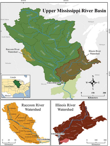
Three different-sized river watersheds: the Raccoon River Watershed (RRW), the Illinois River Watershed (IRW), and the Upper Mississippi River Basin (UMRB), located in the Mississippi River Basin were used to test the MLM approach developed in this study and to explore if the size of a watershed affects the accuracy of MLM. The UMRB covers an area of ~492 000 km², while the IRW and the RRW cover areas of 74 677 and 9400 km², respectively (Fig. 1). Since the objective of this study is to assess the efficiency of MLM by comparing it with results from previous researches, the availability of previous hydrological modeling study was a factor for the selection of these study sites. Better performance of streamflow simulation from the MLM is expected for the larger watershed (e.g. UMRB) compared to the smaller watershed (e.g. RRW), this could be due to limitation of the low spatial resolution of the remote sensing data and temporal scale (i.e. monthly) of the MLM. There are quite significant dams, river diversions, and similar activities occur along the tributaries and main Mississippi River in the study area. As a result, significant human influences, due to dams, reservoirs, diversions, etc., are expected to cause uncertainty in the model. The proposed MLM is not factoring the human impact, model forcings are mainly natural. In this study, the term “watershed” was used if all the study sites are mentioned collectively. Otherwise, we used basin for the Upper Mississippi River (large in size), while watershed for both Illinois and Raccoon Rivers.

Figure 1. Map of the study area showing the Upper Mississippi River Basin (top) and its subwatersheds (bottom left and right). Stars indicate streamflow gauging stations used in this study. Note that the subwatershed downstream of the gauging stations are excluded in the models (shown by lighter colors). The sub-watershed IDs are labelled according to USGS Watershed Boundary Dataset (WBD) Hydrologic Units (HU). USGS gauge numbers are given for the watershed outlets.

2.1 Upper Mississippi River Basin (UMRB)

The UMRB is one of the major sub-basins of the Mississippi River Basin (MRB) which is the largest river basin in North America. The UMRB includes significant parts of Illinois, Iowa, Minnesota, Missouri, and Wisconsin and small parts of Indiana, Michigan, and South Dakota with underlying glacial aquifer system (Fig. 1). Over 30 million residents live in this region and rely on river water and discharge that has significantly increased due to land cover/land use changes cause by farming such as an expansion of soybean/corn fields (Schilling et al. 2010, Srinivasan et al. 2010, NRCS 2010). Understanding and quantifying factors affecting streamflow have ecological and agricultural benefits as it is significantly related to nutrient delivery processes (Schilling et al. 2010). Deciduous forest (19.4%), corn-soybean (33.9%), hay (11.5%), developed area (8.4%), the other cultivated crop (7.5%), pasture (4.9%), open water (2.8%), and grassland herbaceous (2.8%) characterize the land use in the UMRB (Srinivasan et al. 2010). Soil leaching potential and soil runoff potential varies spatially according to various soil types and surface slope (NRCS 2010). The annual precipitation ranges from 980 to 1150 mm/year, and the average LST is between 9°C and 13°C for the 5-year period (Table 1).

Table 1. Summary of watershed characteristics of the study sites.

Name	HU Code	No. of HUs	Average size of HUs	Modeled area	Avg. LST	Max. LST	Min. LST	Ave precipitation
			(km^2)	(km^2)	(°C)	(°C)	(°C)	(mm/year)
UMRB	6	15	29,851	447 771	8.61	26.14	–16.52	989
IRW	8	18	4,008	72 144	11.66	27.88	–14.82	1086
RRW	10	24	370	8 871	10.44	27.68	–15.00	972.67

UMRB: Upper Mississippi River Basin; IRW: Illinois River Watershed; RRW: Raccoon River Watershed. HU: hydrological unit; LST: land surface temperature.

The socio-economic and geographical importance of the MRB and UMRB have gained attention among researchers; as a result, many studies have been conducted in the region, including large projects such as the World Climate Research Programme Global Energy and Water Cycle Experiment (GEWEX) and the Continental-Scale International Project (GCIP) with the long-term goal of demonstrating skill in predicting changes in water resources at various timescales (Maurer and Lettenmaier 2003). These previous studies are mainly based on process-based modeling approaches using the SWAT model (Arnold et al. 2000, Jha et al. 2004, 2006, Gassman et al. 2006, Srinivasan et al. 2010). For example, Arnold et al. (2000) used SWAT to estimate baseflow and groundwater recharge; Jha et al. (2004, 2006) used it to conduct climate change sensitivity assessment of streamflow, while Srinivasan et al. (2010) estimated hydrological budget and crop yield prediction in ungauged perspective by using SWAT with spatial data (e.g. DEM, land use). Several other conceptual and empirical approaches using rainfall–runoff modeling have been conducted in the area (Liston et al. 1994, Maurer and Lettenmaier 2003, Perrin et al. 2007).

2.2 Illinois River Watershed (IRW)

The IRW (Fig. 1, bottom right) drains an area of approx. 75 000 km², which is 44% of the Illinois State land. This watershed comprises 46% of agricultural land in Illinois State, 28% of its forest, 37% of the surface waters, and 95% of urban areas (USACE 2006). Due to extensive development in this region, most prairies and forests have disappeared. Currently, the largest land use in the IRW is agriculture (64%) and the rest is made up of grassland (17%), forest (10%), urban (5%), and water and wetlands (4%) (Demissie et al. 2006, USACE 2006). The average annual air temperature over the last 10 years is approx. 11.5°C, and the average annual precipitation is 1050 mm/year, with warm (23–24°C) and wet summers (June, July, and August; monthly average precipitation: 90–130 mm), and cold (–4°C to 1°C) and relatively dry winters (December, January, and February; monthly average precipitation: 40–120 mm) (Illinois Climate Network 2015) (Table 1). The dominant soil types are mollisols and alfisols with some entisols and inceptisols, which are underlain by the glacial aquifer system. Land-use changes and widening urban areas in this region have caused more rapid streamflow responses during storm events, increasing erosive force, and decreasing baseflow (USACE 2006) that may exacerbate the problems of streamflow and ecological management.

2.3 Raccoon River Watershed (RRW)

The RRW (Fig. 1, bottom left) is located in the western section of the UMRB and encompasses approx. 9400 km² of prime agricultural land in west-central Iowa. This consists of cropland (75.3%), grassland (16.3%), forest (4.4%), and urban (4.0%) areas (Jha et al. 2007). As with most of the agricultural Midwest, land use in the watershed has changed significantly, and this can affect streamflow responses (Schilling et al. 2008). The average annual precipitation ranges between 860 and 1070 mm/year and the mean surface temperature falls between 9.5°C and 11°C (Table 1).

3 Methods and data

3.1 Data sources and processing

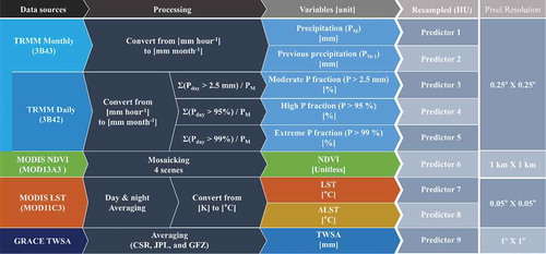
Considering data availability and spatial resolution, various remote sensing-based and other spatial datasets that control the streamflow processes of a watershed were collected for this study. First, the study used 14 watershed variables including TWSA, LST, change in LST (ΔLST), normalized difference vegetation index (NDVI), plant canopy water, soil moisture, snow water equivalent, humidity, wind speed, precipitation (P), previous month precipitation (P_M−1), and a fraction of amount of precipitation for wet (daily P > 2.5 mm; this is the daily median precipitation), extreme (P > 90%), and very extreme (P > 99%) conditions for each watershed. Variable importance analysis showed that variables such as plant canopy water, soil moisture, snow water equivalent, humidity, and wind speed have insignificant roles in simulating streamflow using MLM. Thus, the less important variables were excluded and only nine important variables were used as input variables in the final MLM to simulate streamflow. Various remote sensing data such as TRMM, MODIS NDVI, MODIS LST, and GRACE TWSA (Fig. 2) products were processed and resampled according to the hydrological units (HUs) of the study sites (Fig. 1). The sample size is bounded by the availability of GRACE data, which ranges from April 2002 to July 2016. This range is divided into two datasets: training (November 2004–July 2016; sample size: 142) and testing (April 2002–October 2004; sample size: 30). A brief description of each remote sensing variable/dataset is given below.

Figure 2. Summary of data sources and processing applied on the dataset used in the MLM. Processed variables were resampled according to the HUs of each study site.

3.1.1 Terrestrial water storage anomaly (TWSA)

The GRACE TWSA represents water storage changes on the surface and in the subsurface that potentially explain changes in streamflow due to groundwater (baseflow). GRACE TWSA can provide first-hand information on water storage anomaly directly linked to the water balance of a hydrologic system (Seyoum and Milewski 2016). The GRACE mission consists of two identical satellites that have 500 km orbit altitude and are separated by 220 km (Steitz et al. 2002). The K-band ranging system provides precise (within 1 micron or the width of a human hair) measurements of the distance change between the two satellites, which can be calculated to fluctuations in Earth’s gravity field (Steitz et al. 2002). Most of the GRACE TWSA is related to the fluctuations of TWS after atmospheric effect (mass change caused by atmospheric pressure variation) is removed (Landerer and Swenson 2012). Three solutions of the RL-05 gridded (1°× 1°; ~100 km × 100 km) level-3 GRACE data from three processing centers (the Center for Space Research at the University of Texas, Austin, TX, USA; CSR; the NASA Jet Propulsion Laboratory, CA, USA, JPL; and the GeoforschungsZentrum Potsdam, Germany, GFZ) were downloaded, restored by multiplying the scaling factor, and ensembled (averaged) to ensure the highest level of accuracy. The data are provided by the NASA MEaSUREs Program.¹

3.1.2 Precipitation (P)

The Tropical Rainfall Measurement Mission (TRMM) 3B43 and 3B42 products that contain monthly (3B43) and daily (3B42) precipitation data with global (from the Equator to mid-latitudes; 50°N–50°S) coverage were used in the MLM. The TRMM provides rainfall estimation products based on precipitation rate retrieved by spaceborne sensors, such as microwave imager, precipitation radar, and visible-infrared scanner (Kummerow et al. 1998). Cumulative monthly (mm/month) and daily (mm/d) precipitation data were used in the analysis. The spatial resolution of the data is 0.25°× 0.25° (~27.8 km × 27.8 km). Various precipitation indices recommended by the Expert Team on Climate Change Detection and Indices (ETCCDI) and others (Zhang et al. 2011), such as the fraction of total monthly precipitation, calculated using the number of days greater than conditions of median precipitation (P ~ 2.5 mm), very wet days (P > 90%), and extremely wet days (P > 99%) in a month, were used in the MLM. In addition, one month-lagged precipitation (P_M−1) was used as a training variable in the MLMs to take into account the time of concentration of the watersheds. Calibration and uncertainty of precipitation data from TRMM have been widely conducted and the effectiveness of the data also tested in hydrological models (Adler et al. 2001, Tobin and Bennett 2010, Zhao et al. 2015, Milewski et al. 2015, Beck et al. 2017). TRMM data are available from the NASA Giovanni (Geospatial Interactive Online Visualization ANd aNalysis Infrastructure) service.²

3.1.3 Land surface temperature (LST)

The Moderate Resolution Imaging Spectroradiometer (MODIS) LST (MOD11C3: MODIS/Terra Land Surface Temperature and Emissivity Monthly L3 Global 0.05Deg CMG) product was processed and used in the models. This variable is related to ET – the main component of the water balance that controls streamflow processes. The product is monthly composited average, derived from the MOD11C1 daily LST with 0.05°× 0.05° (~5.6 km × 5.6 km) resolution (Wan et al. 2015). Version 4 products (V4 and V41) were used in this study, as the latest version (V5) may underestimate LST in heavy aerosol conditions due to its algorithm, which is based on longer wavelength bands (Wan 2008, Hulley and Hook 2009). Night and day images are averaged to represent the overall monthly temperature of a watershed. Additionally, month-to-month change in LST (ΔLST) was calculated by subtracting the previous month’s LST from that of the current month. The data were obtained from NASA Earthdata Search.³

3.1.4 Vegetation index (VI)

The MODIS vegetation index product (MOD13A3: MODIS/Terra Vegetation Indices Monthly L3 Global 1 km SIN Grid V006) was selected for VI that would be related to ET. The MODIS VI product provides a 16-day composite of monthly normalized vegetation index (NDVI) and has a global coverage with 1 km × 1 km spatial resolution (Didan 2015). Four scenes (h10v04, h10v05, h11v04, h11v05) were used to cover the UMRB. The data downloaded are a monthly composite product, generated from 16-day products that overlap the month and by employing a weighted temporal average. The raw NDVI values averaged over the HUs for each watershed were used directly in the model, with no quality control or cloud cover analysis. Data are available from NASA Earth Data Search.⁴

3.1.5 Streamflow (Q)

The streamflow gauging data from the outlets of study the areas (USGS 0587450, USGS 05586100, and USGS 05484500, see Fig. 1) were collected from the US Geological Survey National Water Information System (NWIS⁵). Streamflow data were used for both training and testing stages. Data sources and processing steps are summarized in Fig. 2.

3.2 Model design

3.2.1 Boosted regression tree (BRT)

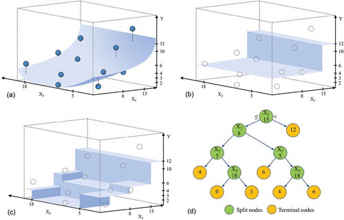
The simulation of monthly streamflow and evaluation of the predictor importance were accomplished using BRT, also known as gradient boosting. BRT is based on a summation of many decision trees partitioning the covariant space by successive binary partitions (Breiman et al. 1984, Friedman et al. 2001). Building a decision tree is a repetitive work to find the best split variable and its split value, based on residual errors. For example, in a multivariate and nonlinear relationship (Fig. 3(a)), a decision tree can be constructed by the following sequences: the best location to divide the surface into the most distinguishable two partitions is X₁ = 15 and it will be assigned as the first spit node of the decision tree (Fig. 3(b) and (d)). Mathematically, this means the residual error between the original surface and newly created surface (Fig. 3(b)) is minimum. Then, the next split variable and its value can be found by considering both parts (X₁ > 15 and X₁ ≦ 15) of the original surface. The same iterative works are conducted until a predefined residual error level is accomplished or the maximum number of split nodes is reached (Fig. 3(c,d)). Note that the final fitting surface may still have a residual error that can be reduced by the boosting process.

Figure 3. Decision tree processes (a) showing an example of covariant space where Y (predictand or target) is explained by X1 and X2 (predictors). The covariant space can be approximated by rectangular spaces (b) and (c), each representing the first node and entire nodes of the decision tree (d).

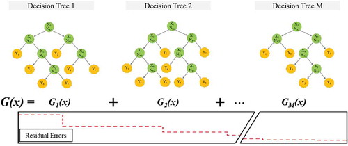
Boosting is based on the observation that finding many rough rules can be a lot easier than finding a single, highly accurate prediction rule (Schapire 2003). In boosting, weak models (decision trees) are fitted iteratively to the residual of training data from the previous models, thereby producing a sequence of weak classifiers (Friedman et al. 2001, Elith et al. 2008). Figure 4 shows a schematic diagram of the boosting process in the BRT. The number of decision trees in boosting is determined by predefined target (goal) residual error and learning rate (residual decrement in each decision tree step).

Figure 4. Schematic diagram of the boosting process in the boosted regression tree (BRT) method.

3.2.2 Training design

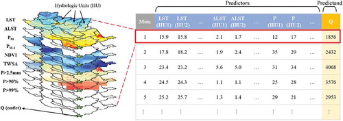
To mimic the relationship between watershed characteristics and streamflow, remote sensing data were aggregated for each sub-watershed (smaller HUs) and used as predictors (Fig. 5). For example, if a watershed has 15 HUs, data for nine predictor variables (see Fig. 2) were extracted for each HU. The total number of predictor variables for that watershed is the number of HUs multiplied by the number of variables (15 × 9). The scale of HU in each watershed was chosen considering the size of the watershed (Fig. 1; Table 1).

Figure 5. Conceptual diagram of the design of training data.

The LS Boost (least-squares regression) algorithm was used to assess residual errors while boosting and the K-fold method was used for cross-validation in the BRT model. During training, model generalization was assessed through cross-validation using the K-fold method. The K-fold method is a cross-validation method that validates a newly trained model using a partitioned dataset. This helps to attenuate overfitting and/or selection bias. The method is a better choice when the size of the training dataset is small. This method randomly divides a dataset into K partitions and the individual partitions are used K – 1 times as part of the training data and one time as the cross-validation data. Consequently, the final model can cover all the observations in the training dataset. To find the best model for each study site, 315 modeling iterations (105 for each watershed) were run by changing the K-fold factor from 2 to 36.

Figure 6 shows a summary of the workflow used in this study. After the training stage, the best model for each study site was selected and tested using independent remote sensing and streamflow data. The performance of MLM, the implications of the results, and the applicability of the method are discussed in the next section.

Figure 6. Workflow and data requirements for training and testing in this study.

3.2.3 Performance evaluation

The performance of the MLM was evaluated statistically using the coefficient of determination (R²), the Nash–Sutcliffe efficiency (NSE), percent bias (PBIAS), and mean absolute error (MAE) by comparing model-estimated data with observed streamflow data. For the equations below, $y_t$ is the observed value at time t, $f_t$ is the simulated (model estimated) value at time t, $\bar{y}$ is the mean of observed values, and $\bar{f}$is the mean of simulated values for the entire evaluation period (T). The R² is computed by Equation (1)(1) $R^2={\left\{\frac{{\sum }_{t=1}^T\left(y_t-\bar{y}\right)\left(f_t-\bar{f}\right)}{{\left[{\sum }_{t=1}^T{\left(y_t-\bar{y}\right)}^2\right]}^{0.5}{\left[{\sum }_{t=1}^T{\left(f_t-\bar{f}\right)}^2\right]}^{0.5}}\right\}}^2$(1) ; it indicates the portion of the variance of data that can be explained by the model, and its value ranges from 0 (no explanation) to 1 (the model explains 100% of the observed data).

(1) $R^2={\left\{\frac{{\sum }_{t=1}^T\left(y_t-\bar{y}\right)\left(f_t-\bar{f}\right)}{{\left[{\sum }_{t=1}^T{\left(y_t-\bar{y}\right)}^2\right]}^{0.5}{\left[{\sum }_{t=1}^T{\left(f_t-\bar{f}\right)}^2\right]}^{0.5}}\right\}}^2$(1)

The NSE (Equation (2)(2) $\mathrm{N}\mathrm{S}\mathrm{E}=1.0--{\sum }_{t=1}^T\frac{{\left({\mathrm{y}}_{\mathrm{t}}‐{\mathrm{f}}_{\mathrm{t}}\right)}^2}{{\sum }_{t=1}^T{\left(y_t-\bar{y}\right)}^2}$(2) ) indicates how a scatterplot of observed versus simulated data fits the 1:1 line; its value ranges from – ∞ to 1, and NSE values close to 1 denote good model performance (Nash and Sutcliffe 1970).

(2) $\mathrm{N}\mathrm{S}\mathrm{E}=1.0--{\sum }_{t=1}^T\frac{{\left({\mathrm{y}}_{\mathrm{t}}‐{\mathrm{f}}_{\mathrm{t}}\right)}^2}{{\sum }_{t=1}^T{\left(y_t-\bar{y}\right)}^2}$(2)

The PBIAS (Equation (3)(3) $\mathrm{P}\mathrm{B}\mathrm{I}\mathrm{A}\mathrm{S}=\left\{\frac{{\sum }_{\mathrm{t}=1}^{\mathrm{T}}\left(y_t--f_t\right)}{{\sum }_{t=1}^{\mathrm{T}}\left(y_{\mathrm{t}}\right)}\right\}\times 100$(3) ) measures the tendency to have a larger or smaller model estimation than the observed data (Moriasi et al. 2007). The optimal value is 0.0, the negative value indicates overestimation, and the positive value indicates underestimation by the model.

(3) $\mathrm{P}\mathrm{B}\mathrm{I}\mathrm{A}\mathrm{S}=\left\{\frac{{\sum }_{\mathrm{t}=1}^{\mathrm{T}}\left(y_t--f_t\right)}{{\sum }_{t=1}^{\mathrm{T}}\left(y_{\mathrm{t}}\right)}\right\}\times 100$(3)

The MAE (Equation (4)(4) $\mathrm{M}\mathrm{A}\mathrm{E}=\frac{{\sum }_{\mathrm{t}=1}^{\mathrm{T}}\left({\mathrm{y}}_{\mathrm{t}}--{\mathrm{f}}_{\mathrm{t}}\right)}{\mathrm{T}}$(4) ) is the average of the difference between simulated and observed values. MAE uses the same unit as the data being used, which helps to understand the scale of the error directly.

(4) $\mathrm{M}\mathrm{A}\mathrm{E}=\frac{{\sum }_{\mathrm{t}=1}^{\mathrm{T}}\left({\mathrm{y}}_{\mathrm{t}}--{\mathrm{f}}_{\mathrm{t}}\right)}{\mathrm{T}}$(4)

In addition, the MLM performance metrics were compared with performance metrics of previous studies conducted in the basin/watersheds using process-based hydrologic modeling approaches. For the Upper Mississippi Basin, a SWAT model-based study conducted by Jha et al. (2006) was used. Jha et al. (2006) simulated UMRB streamflow at daily, monthly, and annual scales using land use, soil type, topography (digital elevation model), daily precipitation, maximum/minimum air temperature, solar radiation, wind speed, and relative humidity data at the 8-digit HU level. They tested the model using data from 1988 to 1997; the test results for monthly streamflow data showed R², NSE, and PBIAS of 0.82%, 0.81%, and 3.9%, respectively.

Similarly, for the Illinois River Watershed, a SWAT model and a Hydrologic and Water Quality System (HAWQS)-based study conducted by Yen et al. (2016) was used to assess the performance of MLM in this watershed. In their study, IRW was modeled using climate, land use, reservoirs, soil type, topography, and water usage data to estimate monthly streamflow, sediment yield, and total nitrogen. Their testing results using data from 1990 to 2001 gave NSE and PBIAS values of 0.72% and 13.91%, respectively.

Lastly, for the Raccoon River Watershed, a SWAT model-based study conducted by Jha et al. (2007) was used. They estimated monthly and annual streamflow, sediment yield, and nitrate of the RRW based on daily precipitation, maximum/minimum air temperature, solar radiation, wind speed, relative humidity, and topography, soil type, fertilizer application rate, land use, and livestock distributions. The testing results using monthly streamflow data from 1993 to 2003 showed R² and NSE values of 0.89 and 0.88, respectively.

4 Results

4.1 Effect of training data partitioning

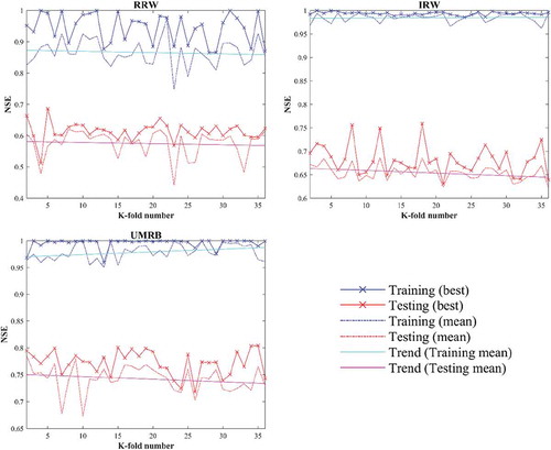
Figure 7 shows the effect of the K-fold factor for each study site in terms of NSE. Overall, the effect of the K-fold number on the performance of the MLMs seems to be insignificant. However, there is a difference in the pattern of NSE with K number between the watersheds. For example, in the RRW MLMs, the NSE values for the training period are not stable compared to those for the IRW and UMRB (Fig. 7, dotted blue lines). The larger fluctuations in NSE values for training in the RRW may imply that the predictor variables do not sufficiently represent the behavior of the streamflow at the outlet for this watershed. This could be due to the size of the RRW, so some of the input data (e.g. GRACE TWSA) have coarse spatial resolution and exceed the size of the watershed. In addition, the rapid streamflow responses of the RRW to storm events may not be well captured at the monthly scale (the temporal resolution of the study).

Figure 7. Streamflow model performance according to K-fold numbers.

4.2 Streamflow modeling

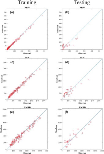
The best three MLMs representing the study sites were selected based on the testing performance of all 315 trained models (Table 2). Overall, the MLMs simulating streamflow fitted the observed streamflow during the training period well. High values of training statistics are expected because the MLM is learning the relationship between predictors and predictand from the given (training) data. However, the testing statistics are expected to be lower than the training because the MLM uses a new set of data (independent dataset) during testing. Figure 8 shows the scatterplots of observed versus simulated streamflow for the RRW, IRW, and UMRB in the training and testing periods. For the training period, the scatterplots show the model simulated streamflow explained the observed data well. All the data are plotted close to the 1:1 line for both low-flow and high-flow conditions. However, for the testing period, the MLM performs better for the large watershed (Fig. 8(f)). We presumed this is due to the limitations of timescale (monthly) and spatial resolution (e.g. GRACE TWSA) of the predictor variables in a small watershed. Furthermore, in the smaller watersheds, the effect of precipitation could not be well captured at a monthly timescale due to the more rapid streamflow response to precipitation in such watersheds.

Table 2. Performance metrics for training and testing.

Site	Mean Q (m^3/s)	K-fold	Training				Testing
			NSE	R^2	PBIAS (%)	MAE (m^3/s)	NSE	R^2	PBIAS (%)	MAE (m^3/s)
RRW	71.16	5	0.99	0.99	5.56 × 10^−5	5.48	0.69	0.71	5.81	23.67
IRW	760.60	18	0.98	0.98	1.75 × 10^−4	61.45	0.76	0.80	−10.96	186.28
UMRB	3791.16	35	0.96	0.96	2.05 × 10^−8	383.46	0.80	0.82	−9.28	773.92

NSE: Nash–Sutcliffe efficiency; R2: coefficient of determination; PBIAS: percent bias; MAE: mean absolute error.

Figure 8. Scatterplots of model-simulated vs observed streamflow for training: (a) RRW, (c) IRW, and (e) UMRB; and testing: (b) RRW, (d) IRW, and (f) UMRB.

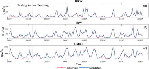
Figure 9 shows time-series plots of observed vs simulated streamflow for each watershed. The MLM for the smaller watershed (RRW) simulates streamflow in the training period perfectly well; however, in the testing period; there are relatively large underestimations and overestimations of peak flows. This implies the MLM of RRW at a monthly timescale could not capture some short-term (storm) events that affect streamflow considerably. On the other hand, the MLM of the UMRB shows relatively constant patterns between simulated and observed streamflow throughout the study period. However, it also has slight overestimations under low streamflow conditions (winter), while underestimations occurred under high streamflow conditions (spring-summer).

Figure 9. Time series plots of model-simulated streamflow and observed streamflow for the entire study period for (a) UMRB, (b) IRW, and (c) RRW.

4.3 Variable contributions

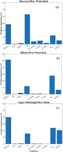
The BRT model provides predictor importance (PI) analysis in terms of mean squared error (MSE) by considering how often a variable is selected to split individual trees in the BRT model. In order to bring the calculated PI to the same scale, a relative PI was calculated and plotted as a percentage (Fig. 10). In the RRW, the most important predictor was P (42.8%), followed by GRACE TWSA (28.3%), P_M−1 (12.2%), and ΔLST (5.1%); other predictors, such as P > 90%, P > 2.5 mm, P > 99%, NDVI, and LST, gave relative PI values of less than 5%. In the IRW, the most important predictor was GRACE TWSA (51.2%), followed by P_M−1 (27.5%), P (11.8%), and ΔLST (6.2%). In the UMRB, the most important predictor was GRACE TWSA (39.6%), followed by P_M−1 (23.6%), ΔLST (20.0%), and P (15.2%). Variables such as NDVI, P > 2.5 mm, P > 90%, LST, and P > 99% have less than 1% relative PI values. Overall, the relative PI demonstrated that TWSA, P, and P_M−1 are the most important variables.

Figure 10. Relative importance of predictor variables for each watershed: (a) RRW, (b) IRW, and (c) UMRB.

Some sub-watersheds (HUs) seem to influence streamflow simulation more than others. The relative PI aggregated over the sub-watersheds (HUs) showed a few with high relative PI values. Generally, HUs located close to the trunk stream and in the middle part of the watershed and/or major tributaries, e.g. Otter Creek-North Raccoon River (0710000614) in the RRW, Lower Illinois-Senachwine Lake (07130001) in the IRW, and Upper Mississippi-Maquoketa-Plum (070600) in the UMRB (Fig. 11), tend to have high relative importance compared to the HUs located upstream or in tributaries. This indicates that some HUs characterize streamflow patterns at the outlet more than others. Therefore, HUs with low relative PI imply that the remote sensing variables in the area had little or no chance of being selected to explain streamflow responses compared to the dominant variables of the more representative HUs during regression tree construction. For example, in the UMRB, the Lower Illinois (071300) has very low relative PI because most of the streamflow pattern at the outlet is explained by the Upper Illinois (071200). Likewise, in the RRW, the Upper South Raccoon River (0710000704) and its adjacent subwatersheds (0710000703 and 0710000707) which belongs to the South Raccoon River Watershed – the main tributary of the RRW – have high relative PI.

Figure 11. Map showing the relative contribution of sub-watersheds in simulating the MLMs for each watershed. Darker shading shows high relative importance and lighter shading shows low or no importance.

4.4 Comparison with existing process-based model results

Table 3 presents the performance of the MLMs for each watershed compared with the performance of process-based models conducted on the same study sites and from the same gauging stations. Since the studies have variable testing periods, efforts were made to match the testing period of this study (April 2002–October 2004) with those of the previous studies. Due to the lack of overlap in the testing periods between the MLMs in this study and process-based models, a direct comparison is unjust. However, some general advantages and disadvantages between MLM and a process-based approach can be derived from the performance comparison. The process-based approach conducted in a small watershed (e.g. RRW) achieved better performance compared to the MLM in this study. Generally, process-based models are more cost-effective and manageable for small watersheds like the RRW; thus, uncertainties from the input data are low and the model set-up, processing, and calibration are relatively efficient. However, for large watersheds (e.g. IRW and UMRB), the watershed size and heterogeneity make process-based modeling less manageable and more difficult to build in an efficient manner. This is due to the high data demand, and the required effort of data collection may extensively increase. As a result, uncertainties from data, processing, and calibration become considerable. Conversely, the remote sensing data based MLM introduced in this study may give better performance in large watersheds, as these are developed using publicly accessible data and a cost-effective and manageable method. Considering the streamflow model performance of the IRW and UMRB, the remote sensing-based MLM looks competitive against the conventional process-based approaches. It is important to note the superiority of process-based models over the MLM in areas where (a) understanding of specific hydrologic processes (e.g. infiltration) is needed, (b) hydrologic variables need to be determined anywhere in the watershed (e.g. spatial variation of soil moisture), and (c) the study requires prediction of future conditions that are different from those for which the model was developed (e.g. prediction of runoff due to land-use change).

Table 3. Comparison of streamflow estimation performances between existing process-based model results (SWAT) and machine learning modellng (MLM) for each study site.

Site	Process-based model				MLM (this study)
	Reference	Validation (testing) period	NSE	PBIAS	NSE	PBIAS
RRW	Jha et al. (2007)	1993–2003	0.88	-	0.69	5.81%
IRW	Yen et al. (2016)	1990–2001	0.72	13.91%	0.76	–10.96%
UMRB	Jha et al. (2006)	1988–1997	0.81	3.9%	0.80	–9.28%

Note: The testing period for the MLM is 2002–2004. RRW: Raccoon River Watershed; IRW: Illinois River Watershed; UMRB: Upper Mississippi River Basin. NSE: Nash–Sutcliffe efficiency; PBIAS: percent bias.

5 Discussion

Monthly streamflow was simulated using a remote sensing-based MLM for different-sized watersheds (the RRW, the IRW, and the UMRB). For the model training phase, a semi-distributed approach was applied to capture the contribution of each sub-watershed, and an iterative K-fold cross-validation was conducted to find the optimal K number. The analysis showed that the performance of the MLM is insensitive to K number.

In the testing period, the RRW model under (over)-predicted peak flows, while the IRW and the UMRB models showed better fits to the observed streamflow. The MLMs performed better for both the IRW and UMRB compared to the smaller watershed, the RRW. This could be due to the coarse spatial resolution of the GRACE data and low temporal resolution (monthly) used in the simulations. For the RRW, the time of concentration of runoff is relatively shorter compared to the large IRW or the UMRB. As a result, in response to precipitation events, streamflow fluctuates rapidly (in days) at the outlet for the case of the RRW. Thus, monthly timescale MLM is less likely to capture the streamflow variability. Similarly, a single GRACE pixel characterizes the entire RRW (no variation of TWSA spatially), so GRACE accuracy is very limited at this watershed scale. Further, a significant drop in test statistics observed compared to the statistics in the training period. This is partly due to expected overfitting from the MLM (BRT method). During model development, measures were taken to reduce the effect of overfitting, for example, by reducing the number of predictor variables. In addition, the sample size (limited by GRACE sample size) plays a role. As sample size increases (more GRACE data are available), model performance is expected to improve.

Relative predictor importance (PI) results showed GRACE TWSA, P, and P_M−1 are the most important predictor variables. GRACE TWSA plays the most important role in the IRW and UMRB models, and the second most important role in the RRW model. This generally emphasizes the effectiveness of GRACE data for streamflow modeling. The relative importance of these two variables depends on the watershed size. For example, GRACE TWSA (which has high accuracy at a large scale) plays the most important role in the larger watersheds (the IRW and UMRB models); however, P is the most important predictor variable in the RRW model. The relative contribution of the previous month’s precipitation (P_M−1) tends to increase as the watershed size increases. This is consistent with the expected longer time of concentration for larger watersheds where precipitation that occurs in the upstream areas will take a longer time to reach the outlet. A relatively higher predictor importance of derivative P data such as the fraction of moderate, high, and extreme precipitation (P > 2.5 mm, P > 90%, and P > 99%) in the RRW implies that the streamflow of the small watershed is more sensitive to the magnitude of extreme precipitation events.

The LST and ΔLST were expected to explain the timing of snow melting, ET processes, and other variables (e.g. soil moisture, wind speed, humidity) indirectly. The relative PI shows that ΔLST seems to be a more important predictor variable than LST. ΔLST is significant in that a large magnitude of ΔLST indicates season change. This is important in simulating seasonally induced streamflow such as an increase in discharge in early spring driven by snow melting or low flow in late summer caused by high temperatures and ET. Furthermore, ΔLST overwhelms NDVI, which is expected to account for the ET processes. The low relative PIs of LST and NDVI indicate that the variables have minimum effect on streamflow or they had no chance to be used in a decision tree because the other predictors such as TWSA and ΔLST explain most of the streamflow responses.

The scales of sub-watersheds used in the UMRB, IRW, and RRW models – HU levels, HU-6, HU-8, and HU-10, respectively – are larger than those used in process-based studies. The HU scales were chosen to keep an appropriate and manageable number of predictor variables for each watershed; however, this may be one of the reasons that the MLMs of UMRB and RRW have lower testing performance than the process-based models. Testing of a finer level of HUs is recommended to test this hypothesis. Moreover, the comparison of testing performance between process-based approaches and MLMs in this study is not based on the same period.

This method has advantages to simulate streamflow for large watersheds without any in-situ watershed information. However, some limitations should be considered before applying the remote sensing-based MLM approach to other areas: (a) in-situ streamflow data are necessary for the training dataset, (b) temporal applicability is limited by the temporal resolution of the remote sensing data such as GRACE, (c) the PI of the MLM may not necessarily be a reflection of the real characteristics of a watershed, and (d) the MLM is only suitable for prediction of streamflow at the outlet. Like process-based models, without modification of the MLM set-up in this study, it is not applicable to estimate flow anywhere within the watershed.

One of the applications of this remote sensing-based MLM is flood prediction. However, the following limitations need to be addressed: (i) variables at a finer temporal resolution such as daily data should be used during model construction since streamflow responses to extreme precipitation are more likely to occur in a short timescale; and (ii) GRACE TWSA (only available at a monthly timescale) may be replaced by antecedent precipitation data, which is expected to improve model performance.

6 Conclusions

The study presented a remote sensing-based MLM (machine learning modeling) that simulates monthly streamflow with comparable performance relative to an in-situ-based distributed hydrologic model. The effectiveness of remote sensing-based MLM depends on the watershed size and is limited by the spatial resolution of the input data, such as GRACE. However, research has shown that downscaling of GRACE data is possible (Seyoum et al. 2019, Shang et al. 2019, Milewski et al. 2019b); thus, better results can be achieved in small watersheds if such data are used. We drew the following important conclusions from this study:

• The remote sensing-based MLM potentially has advantages for simulating streamflow for large watersheds such as the IRW and UMRB, compared to process-based models in terms of data acquisition effort, computing resources, and model performance.

• The distributed approach and predictor importance (PI) analysis demonstrate the most representative sub-watersheds in the streamflow responses. This information can be used to establish an efficient water resource management policy in terms of land use and water usage.

• The efficiency of the MLM is determined by TWSA and performance can be improved if better quality TWSA or TWSA-related data are used.

• The importance of P_M−1 implies that the aggregated antecedent precipitation conditions have the potential to be used instead of GRACE TWSA. This supports the most recent machine learning-based streamflow modeling approaches, such as Long Short-Term Memory (LSTM) network.

• ΔLST can be used in MLM to reflect, indirectly, seasonal changes such as snow melting, and ET-related climatic effects, such as humidity and wind speed, which cannot be easily acquired by remote sensing.

• The BRT model can be trained based on a limited amount of data (142 months) and performs well for monthly streamflow simulations. Thus, the model may be applicable for watersheds where streamflow gauge data are limited and sparse.

The remote sensing-based MLM introduced in this study has the potential to be a supplementary and popular approach in simulating streamflow. Overall model performance is comparable with that of process-based approaches, but with significantly less modeling effort. Remote sensing-based MLM has the potential to be a very attractive tool in estimating streamflow for watersheds that have not been sufficiently studied in a hydrologic and geologic manner.

Acknowledgements

This work was supported in part by the College of Arts and Sciences, Illinois State University.

Disclosure statement

No potential conflict of interest was reported by the authors.

Notes

¹ https://grace.jpl.nasa.gov/data/get-data/monthly-mass-grids-land/(Date accessed: 1 September 2017).

² https://giovanni.gsfc.nasa.gov/giovanni/(Date accessed: 26 September 2017).

³ https://search.earthdata.nasa.gov/(Date accessed: 31 August 2017).

⁴ https://search.earthdata.nasa.gov/(Date accessed: 28 August 2017).

⁵ https://waterdata.usgs.gov/nwis (Date accessed: 9 November 2018).

References

- Adler, R.F., et al. 2001. Intercomparison of global precipitation products: the third Precipitation Intercomparison Project (PIP-3). Bulletin of the American Meteorological Society, 82 (7), 1377–1396. doi:10.1175/1520-0477(2001)082<1377:IOGPPT>2.3.CO;2
- Ahmad, S., Kalra, A., and Stephen, H., 2010. Estimating soil moisture using remote sensing data: A machine learning approach. Advances in Water Resources, 33 (1), 69–80. doi:10.1016/j.advwatres.2009.10.008
- Arnold, J.G., et al. 2000. Regional estimation of base flow and groundwater recharge in the Upper Mississippi river basin. Journal of Hydrology, 227 (1–4), 21–40. doi:10.1016/S0022-1694(99)00139-0
- Bajwa, S. and Vibhava, V., 2009. A distributed artificial neural network model for watershed-scale rainfall-runoff modeling. Transactions of the ASABE, 52 (3), 813–823. doi:10.13031/2013.27402
- Beck, H.E., et al. 2017. Global-scale evaluation of 22 precipitation datasets using gauge observations and hydrological modeling. Hydrology and Earth System Sciences, 21 (12), 6201–6217. doi:10.5194/hess-21-6201-2017
- Beven, K.J., 2011. Rainfall-runoff modeling: the primer. Chichester, UK: John Wiley & Sons.
- Blöschl, G., 2005. Rainfall‐runoff modeling of ungauged catchments. In: M.G. Anderson, ed. Encyclopedia of hydrological sciences. New York: John Wiley, Wiley Online Library.
- Boegh, E., et al. 2009. Remote sensing based evapotranspiration and runoff modeling of agricultural, forest and urban flux sites in Denmark: from field to macro-scale. Journal of Hydrology, 377 (3), 300–316. doi:10.1016/j.jhydrol.2009.08.029
- Bourdin, D.R., Fleming, S.W., and Stull, R.B., 2012. Streamflow modeling: a primer on applications, approaches and challenges. Atmosphere-Ocean, 50 (4), 507–536. doi:10.1080/07055900.2012.734276
- Brakenridge, G.R., et al., 2005. Space‐based measurement of river runoff. EOS, Transactions American Geophysical Union, 86 (19), 185–188.
- Breiman, L., et al., 1984. Classification and regression trees. New York: Taylor & Francis.
- Chang, W. and Chen, X., 2018. Monthly rainfall-runoff modeling at watershed scale: A comparative study of data-driven and theory-driven approaches. Water, 10 (9), 1116. doi:10.3390/w10091116
- Chen, J.M., et al., 2005. Distributed hydrological model for mapping evapotranspiration using remote sensing inputs. Journal of Hydrology, 305 (1), 15–39.
- Chen, X.-Y., Chau, K.-W., and Wang, W.-C., 2015. A novel hybrid neural network based on continuity equation and fuzzy pattern-recognition for downstream daily river discharge forecasting. Journal of Hydroinformatics, 17 (5), 733–744. doi:10.2166/hydro.2015.095
- Chiew, F., Stewardson, M., and McMahon, T., 1993. Comparison of six rainfall-runoff modeling approaches. Journal of Hydrology, 147 (1–4), 1–36. doi:10.1016/0022-1694(93)90073-I
- Cisneros, J., 2014. Freshwater resources. In: C.B. Field, et al., eds.. Climate change: impacts, adaptation, and vulnerability. Part A: global and sectoral aspects. Contribution of working group II to the fifth assessment report of the intergovernmental panel on climate change. Cambridge, United Kingdom: Cambridge University Press, 1–1150.
- Dawson, C.W. and Wilby, R., 1998. An artificial neural network approach to rainfall-runoff modeling. Hydrological Sciences Journal, 43 (1), 47–66. doi:10.1080/02626669809492102
- Demissie, M., et al. 2006. Evaluating the effectiveness of the Illinois River conservation reserve enhancement program in reducing sediment delivery. IAHS Publication, 306, 295.
- Deo, R.C. and Şahin, M., 2016. An extreme learning machine model for the simulation of monthly mean streamflow water level in eastern Queensland. Environmental Monitoring and Assessment, 188 (2), 90. doi:10.1007/s10661-016-5094-9
- Dhi, D., 2003. Mike-11: a modeling system for rivers and channels, reference manual. Horsholm, Denmark: DHI–Water and Development.
- Didan, K., 2015. MOD13A3: MODIS/terra vegetation indices monthly L3 global 1km SIN grid V006. NASA EOSDIS Land Processes DAAC, 10. https://ind01.safelinks.protection.outlook.com/?url=https%3A%2F%2Fdoi.org%2F10.5067%2FMODIS%2FMOD13A3.006&data=02%7C01%7Csathyan.dhanasekaran%40integra.co.in%7C1a7ea24f2b7b4345260808d82e593d25%7C70e2bc386b4b43a19821a49c0a744f3d%7C0%7C0%7C637310308167990088&sdata=imXUUikZ5AV%2B8QOy6x%2FeMaVgTwD7NOhmoViY3v0YZ4A%3D&reserved=0 [Accessed 15 Sept 2018].
- Elith, J., Leathwick, J.R., and Hastie, T., 2008. A working guide to boosted regression trees. Journal of Animal Ecology, 77 (4), 802–813. doi:10.1111/j.1365-2656.2008.01390.x
- Friedman, J., Hastie, T., and Tibshirani, R., 2001. The elements of statistical learning. New York: Springer series in statistics.
- Gassman, P.W., et al., 2006. Upper Mississippi River Basin modeling system part 1: SWAT input data requirements and issues. In: V.P. Singh and Y.J. Xu, eds. Coastal Hydrology and Processes. Highlands Ranch, USA: Water Resources Publications, LLC, 103–115.
- Herschy, R.W., 2009. Streamflow measurement. 3rd ed. New York: Taylor & Francis.
- Hong, Y., et al., 2007. A first approach to global runoff simulation using satellite rainfall estimation. Water Resources Research, 43 (8). doi:10.1029/2006WR005739
- Hsu, K.L., Gupta, H.V., and Sorooshian, S., 1995. Artificial neural network modeling of the rainfall‐runoff process. Water Resources Research, 31 (10), 2517–2530. doi:10.1029/95WR01955
- Hulley, G.C. and Hook, S.J., 2009. Intercomparison of versions 4, 4.1 and 5 of the MODIS land surface temperature and emissivity products and validation with laboratory measurements of sand samples from the Namib desert, Namibia. Remote Sensing of Environment, 113 (6), 1313–1318. doi:10.1016/j.rse.2009.02.018
- Illinois Climate Network, 2015. Water and atmospheric resources monitoring program. Champaign, IL: Illinois State Water Survey.
- Jha, M., et al., 2004. Impacts of climate change on streamflow in the Upper Mississippi River Basin: A regional climate model perspective. Journal of Geophysical Research: Atmospheres, 109 (D9). doi:10.1029/2003JD003686
- Jha, M., et al. 2006. Climate change sensitivity assessment on Upper Mississippi River Basin streamflows using SWAT 1. JAWRA Journal of the American Water Resources Association, 42 (4), 997–1015. doi:10.1111/j.1752-1688.2006.tb04510.x
- Jha, M.K., Gassman, P.W., and Arnold, J.G., 2007. Water quality modeling for the Raccoon River watershed using SWAT. Transactions of the ASABE, 50 (2), 479–493.
- Khosravi, K., Mirzai, H., and Saleh, I., 2013. Assessment of empirical methods of runoff estimation by statistical test (Case study: Banadaksadat Watershed, Yazd Province). International journal of Advanced Biological and Biomedical Research 1 (3), 1–17.
- Kratzert, F., et al., 2018. Rainfall-runoff modeling using long short-term memory (LSTM) networks. Earth Syst. Sci., 22, 6005–6022. https://ind01.safelinks.protection.outlook.com/?url=https%3A%2F%2Fdoi.org%2F10.5194%2Fhess-22-6005-2018&data=02%7C01%7Csathyan.dhanasekaran%40integra.co.in%7C1a7ea24f2b7b4345260808d82e593d25%7C70e2bc386b4b43a19821a49c0a744f3d%7C0%7C0%7C637310308167990088&sdata=uNw5vmd7GjgJc%2FXlOiSBDHNnaTwyyXrtitj2voTFnIw%3D&reserved=0
- Kummerow, C., et al. 1998. The tropical rainfall measuring mission (TRMM) sensor package. Journal of Atmospheric and Oceanic Technology, 15 (3), 809–817. doi:10.1175/1520-0426(1998)015<0809:TTRMMT>2.0.CO;2
- Landerer, F.W. and Swenson, S.C., 2012. Accuracy of scaled GRACE terrestrial water storage estimates. Water Resources Research, 48 (4). doi:10.1029/2011WR011453
- Liston, G., Sud, Y., and Wood, E., 1994. Evaluating GCM land surface hydrology parameterizations by computing river discharges using a runoff routing model: application to the Mississippi basin. Journal of Applied Meteorology, 33 (3), 394–405. doi:10.1175/1520-0450(1994)033<0394:EGLSHP>2.0.CO;2
- Liu, T., et al., 2012. On the usefulness of remote sensing input data for spatially distributed hydrological modeling: case of the Tarim River basin in China. Hydrological Processes, 26 (3), 335–344.
- Mahmoud, S.H., 2014. Investigation of rainfall–runoff modeling for Egypt by using remote sensing and GIS integration. Catena, 120, 111–121.
- Markstrom, S.L., et al., 2015. PRMS-IV, the precipitation-runoff modeling system, version 4. Reston, VA: US Geological Survey Techniques and Methods. (6-B7).
- Maurer, E.P. and Lettenmaier, D.P., 2003. Predictability of seasonal runoff in the Mississippi River basin. Journal of Geophysical Research: Atmospheres, 108, D16.
- Melesse, A.M. and Graham, W.D., 2004. Storm runoff prediction based on a spatially distributed travel time method utilizing remote sensing and GIS. JAWRA Journal of the American Water Resources Association, 40 (4), 863–879. doi:10.1111/j.1752-1688.2004.tb01051.x
- Milewski, A., et al. 2019a. Multi-scale hydrologic sensitivity to climatic and anthropogenic changes in Northern Morocco. Geosciences, 10 (1), 13. doi:10.3390/geosciences10010013
- Milewski, A., Elkadiri, R., and Durham, M., 2015. Assessment and intercomparison of TMPA satellite precipitation products in varying climatic and topographic regimes. Remote Sensing, 7 (5), 5697–5717. doi:10.3390/rs70505697
- Milewski, M.A., et al., 2019b. Spatial downscaling of GRACE TWSA data to identify spatiotemporal groundwater level trends in the Upper Floridan Aquifer, Georgia, USA. Remote Sensing, 11 (23), 2756.
- Milly, P.C., Dunne, K.A., and Vecchia, A.V., 2005. Global pattern of trends in streamflow and water availability in a changing climate. Nature, 438 (7066), 347–350. doi:10.1038/nature04312
- Minns, A. and Hall, M., 1996. Artificial neural networks as rainfall-runoff models. Hydrological Sciences Journal, 41 (3), 399–417. doi:10.1080/02626669609491511
- Moriasi, D.N., et al. 2007. Model evaluation guidelines for systematic quantification of accuracy in watershed simulations. Transactions of the ASABE, 50 (3), 885–900. doi:10.13031/2013.23153
- Mutlu, E., et al. 2008. Comparison of artificial neural network models for hydrologic predictions at multiple gauging stations in an agricultural watershed. Hydrological Processes, 22 (26), 5097–5106. doi:10.1002/hyp.7136
- Nash, J.E. and Sutcliffe, J.V., 1970. River flow forecasting through conceptual models part I—A discussion of principles. Journal of Hydrology, 10 (3), 282–290. doi:10.1016/0022-1694(70)90255-6
- Neitsch, S.L., et al., 2011. Soil and water assessment tool theoretical documentation version 2009. College Station, TX: Texas A & M University, Texas Water Resources Institute Technical Report No. 406.
- NRCS, 2010. Assessment of the effects of conservation practices on cultivated cropland in the upper Mississippi River basin. Washington, D.C.: US Department of Agriculture, Natural Resources Conservation Service.
- Perrin, C., et al. 2007. Impact of limited streamflow data on the efficiency and the parameters of rainfall—runoff models. Hydrological Sciences Journal, 52 (1), 131–151. doi:10.1623/hysj.52.1.131
- Rajurkar, M., Kothyari, U., and Chaube, U., 2002. Artificial neural networks for daily rainfall—runoff modeling. Hydrological Sciences Journal, 47 (6), 865–877. doi:10.1080/02626660209492996
- Riad, S., et al. 2004. Rainfall-runoff model using an artificial neural network approach. Mathematical and Computer Modeling, 40 (7–8), 839–846. doi:10.1016/j.mcm.2004.10.012
- Schapire, R.E., 2003. The boosting approach to machine learning: an overview. In: D.D Denison, M.H. Hansen, C.C. Holmes, B. Mallick, and B. Yu., eds. Nonlinear estimation and classification. Lecture notes in statistics, vol 171. New York, NY: Springer, 149–171.
- Schilling, K.E., et al., 2008. Impact of land use and land cover change on the water balance of a large agricultural watershed: historical effects and future directions. Water Resources Research, 44 (7). doi:10.1029/2007WR006644
- Schilling, K.E., et al. 2010. Quantifying the effect of land use land cover change on increasing discharge in the Upper Mississippi River. Journal of Hydrology, 387 (3–4), 343–345. doi:10.1016/j.jhydrol.2010.04.019
- Seo, Y., Kim, S., and Singh, V., 2018. Machine learning models coupled with variational mode decomposition: A new approach for modeling daily rainfall-runoff. Atmosphere, 9 (7), 251. doi:10.3390/atmos9070251
- Seyoum, M.W., Kwon, D., and Milewski, M.A., 2019. Downscaling GRACE TWSA data into high-resolution groundwater level anomaly using machine learning-based models in a glacial aquifer system. Remote Sensing, 11 (7), 824. doi:10.3390/rs11070824
- Seyoum, W.M., 2018. Characterizing water storage trends and regional climate influence using GRACE observation and satellite altimetry data in the Upper Blue Nile River Basin. Journal of Hydrology, 566, 274–284. doi:10.1016/j.jhydrol.2018.09.025
- Seyoum, W.M. and Milewski, A.M., 2016. Monitoring and comparison of terrestrial water storage changes in the northern high plains using GRACE and in-situ based integrated hydrologic model estimates. Advances in Water Resources, 94, 31–44. doi:10.1016/j.advwatres.2016.04.014
- Seyoum, W.M. and Milewski, A.M., 2017. Improved methods for estimating local terrestrial water dynamics from GRACE in the Northern High Plains. Advances in Water Resources, 110, 279–290. doi:10.1016/j.advwatres.2017.10.021
- Seyoum, W.M., Milewski, A.M., and Durham, M.C., 2015. Understanding the relative impacts of natural processes and human activities on the hydrology of the Central Rift Valley lakes, East Africa. Hydrological Processes, 29 (19), 4312–4324. doi:10.1002/hyp.10490
- Shang, Q., et al. 2019. Downscaling of GRACE datasets based on relevance vector machine using InSAR time series to generate maps of groundwater storage changes at local scale. Journal of Applied Remote Sensing, 13 (4), 048503. doi:10.1117/1.JRS.13.048503
- Srinivasan, R., Zhang, X., and Arnold, J., 2010. SWAT ungauged: hydrological budget and crop yield predictions in the Upper Mississippi River Basin. Transactions of the ASABE, 53 (5), 1533–1546. doi:10.13031/2013.34903
- Steitz, D., et al., 2002. GRACE launch. Press Kit. Pasadena, CA: Jet Propulsion Laboratory/NASA.
- Tanty, R. and Desmukh, T.S., 2015. Application of artificial neural network in hydrology—A review. International Journal of Engineering Research and Technology, 4, 184–188.
- Taormina, R., Chau, K.-W., and Sivakumar, B., 2015. Neural network river forecasting through baseflow separation and binary-coded swarm optimization. Journal of Hydrology, 529, 1788–1797. doi:10.1016/j.jhydrol.2015.08.008
- Tobin, K.J. and Bennett, M.E., 2010. Adjusting satellite precipitation data to facilitate hydrologic modeling. Journal of Hydrometeorology, 11 (4), 966–978. doi:10.1175/2010JHM1206.1
- Tokar, A.S. and Johnson, P.A., 1999. Rainfall-runoff modeling using artificial neural networks. Journal of Hydrologic Engineering, 4 (3), 232–239. doi:10.1061/(ASCE)1084-0699(1999)4:3(232)
- USACE, 2006. (U.S. Army Corps of Engineers) Illinois River Basin restoration comprehensive plan with integrated environmental assessment, public review draft, February 2006, Rock Island District. Rock Island, IL: USACE.
- Wan, Z., 2008. New refinements and validation of the MODIS land-surface temperature/emissivity products. Remote Sensing of Environment, 112 (1), 59–74. doi:10.1016/j.rse.2006.06.026
- Wan, Z., Hook, S., and Hulley, G., 2015. MOD11C3 MODIS/terra land surface temperature/emissivity monthly L3 global 0.05 deg CMG V006 [Data set]. NASA EOSDIS Land Processes DAAC. https://ind01.safelinks.protection.outlook.com/?url=https%3A%2F%2Fdoi.org%2F10.5067%2FMODIS%2FMOD11C3.006&data=02%7C01%7Csathyan.dhanasekaran%40integra.co.in%7C1a7ea24f2b7b4345260808d82e593d25%7C70e2bc386b4b43a19821a49c0a744f3d%7C0%7C0%7C637310308167990088&sdata=it8TzklPDF9phTnW4r4LdNVmILiVdfwz9dlCqjwd8jE%3D&reserved=0 [Accessed 01 Sept 2018].
- Yaseen, Z.M., et al., 2017. Novel approach for streamflow forecasting using a hybrid ANFIS-FFA model. Journal of Hydrology, 554, 263–276. doi:10.1016/j.jhydrol.2017.09.007
- Yen, H., et al. 2016. Application of large-scale, multi-resolution watershed modeling framework using the Hydrologic and Water Quality System (HAWQS). Water, 8 (4), 164. doi:10.3390/w8040164
- Zhang, X., et al., 2011. Indices for monitoring changes in extremes based on daily temperature and precipitation data. Wiley Interdisciplinary Reviews. Climate Change, 2 (6), 851–870.
- Zhao, H., et al. 2015. Evaluating the suitability of TRMM satellite rainfall data for hydrological simulation using a distributed hydrological model in the Weihe River catchment in China. Journal of Geographical Sciences, 25 (2), 177–195. doi:10.1007/s11442-015-1161-3