Discharge estimation for medium-sized river using multi-temporal remote sensing data: a case study in Brazil

ABSTRACT

The increased availability of remote sensing data associated with good revisit capabilities promotes the use of these data to estimate hydrological variables such as river width. This becomes especially useful for regions with poor coverage of in situ stations. In this study, we propose a methodological approach to estimate river discharge from time series of river width. The discharge from in situ hydrological stations was regionalized to calibrate a series of width-discharge models of three different types using theoretical hydraulic geometry power functions. Our methods used both individual and average width to estimate discharge. It was found that a priori selected average widths yielded models with better adjustment than the systematic average or the individual width approaches. Nearly 70% of the models generated with the selected average widths produced Nash-Sutcliffe efficiency values better than 0.7. The article explores the implications of estimating discharge from width and describes the method used.

KEYWORDS:

• river width
• river discharge
• remote sensing imagery
• hydraulic geometry
• medium-sized river

Editor A. Fiori Associate editor G. Thirel

1 Introduction

Surficial water of fluvial channels constitutes about only 0.49% of the soft water reserves of our planet (Shiklomanov 1993). Despite this apparent scarcity, rivers are the main source of water for our needs, be it urban, industrial or agricultural. In ecological terms, rivers play a capital role in maintaining life of most species of fauna and flora and function as vectors of connectivity and modification between landscapes promoting exchange of matter and energy.

Monitoring river discharge is mostly done by in situ measurements from fixed hydrological stations. This approach is a limiting factor in terms of coverage of the hydrological network in many parts of the world where political, economic and logistical restrictions do not permit a more extensive network of stations (Nace 1964, The Ad Hoc Group et al. 2001, Alsdorf et al. 2007, Pavelsky et al. 2014). Moreover, there has been, in the last few decades, a reduction in the number of in situ stations around the world. The reduction is clearly observable in the data repertory of the Global Runoff Data Centre (GRDC) that publishes water discharge data worldwide (Alsdorf et al. 2007, Pavelsky et al. 2014).

In situ hydrological stations are often ill distributed across continents and watersheds, a fact that can hinder the generation of valid hydrological prediction models. The lack of reliable hydrological data is often a limiting factor (irrigation, energy generation, bridges, canals, etc.). The management of water resource in these conditions can be difficult or impracticable.

The past few years (especially since the implementation of the ESA Copernicus Programme¹) have seen an unprecedented increase in the number of Earth observation satellite missions with free public distribution of data that has motivated many scientific researchers to use remote sensing data for hydrological applications (Wass et al. 1997, Frappart et al. 2005, Chu et al. 2006, Tarpanelli et al. 2013, 2019, Villar et al. 2013, Pekel et al. 2016, de Oliveira et al. 2017). These authors and many more have contributed to proposing and implementing new methods to estimate a number of hydrological variables that can greatly help monitoring the fluvial network and its dynamics. In that sense remote sensing has become an essential tool to systematically monitor water resources in a synoptic manner while reducing cost and logistics of in situ measurements.

It appears that studies involving remote sensing products can be divided into three categories. The first category is characterized by the use of imaging sensors to study the planimetric properties of water or the surrounding land. Some references of such studies are presented in Table 1. These studies usually take advantage of the fact that water absorbs almost all electromagnetic radiation in the near and shortwave infrared portions of the spectrum to either separate the water pixel from the land pixel (e.g. Smith and Pavelsky 2008, Pekel et al. 2016) or to estimate the amount of water in mixed pixel (Tarpanelli et al. 2013, Pôssa and Maillard 2018). In both cases, the idea is to estimate the river width or its impact on the land. The second category is associated with altimetry sensors that can measure elevation from which water level and slope can be estimated. These studies usually combine the altimetry data with some aspect of image data as well (e.g. Tourian et al. 2016, Kim et al. 2019). The third category combines the aspects of the first and second by providing a continuous, description of the topography of the surface in matrix format (raster) such as the Shuttle Radar Topographic Mission (SRTM) or the Global Digital Elevation Model (GDEM) compiled from the ASTER archives. The SWOT (Surface Water and Ocean Topography) satellite mission to be launched in 2022, will fall in this third category by supplying simultaneously a water mask for which every pixel will show elevation.

Table 1. Hydrological variables inferred from satellite images planimetric properties. ACC: accuracy; RMSE: root mean square error; RRMSE: relative root mean square error (divided by mean of observations); r2: coefficient of determination; $y_i$: predicted value, $x_i$: observed value

Estimated variable	Mission	Results	References
Water surface	SPOT Vegetation	ACC = 95.4%	Haas et al. (2009)
	Landsat	ACC = 97%	Mueller et al. (2016)
	Landsat	ACC = 99.2%	Pekel et al. (2016)
Discharge	ERS 1	r2 = 0.83	Smith et al. (1996)
	Quickbird-2	ACC = 97%	Xu et al. (2004)
	Quickbird-2	ACC = 80%	Zhang et al. (2004)
	MODIS	r2 = 0.81	Smith and Pavelsky (2008)
	Landsat	RRMSE 26–41%	Gleason et al. (2014; 2014)
	MODIS	RMSE = 10%	Elmi et al. (2015)
Propagation speed	MODIS	$y_i$ = 1.01 m/s $x_i$ = 0.97 m/s	Smith and Pavelsky (2008)
	MODIS	-	Sichangi et al. (2018)

With the increase in the number of Earth observing missions, the various aspects of hydrometric characteristics of rivers can be studied using data from a wide range of spatial, spectral and temporal resolutions (Jensen 2006, Tang et al. 2009). In particular, the use of synthetic aperture radar (SAR) sensors enables a continuous monitoring in all weather conditions and regardless of solar illumination. The recent Sentinel missions (S1 and S2) of the Global Monitoring for Environment and Security (GMES) already supply valuable data with high spatial (10 m and 20 m) and temporal (5–12 days) resolutions. Sentinel-1 is a twin satellite constellation equipped with a SAR sensor in Band C (λ = 5.6 cm) and a combined revisit frequency of 6–12 days (depending on the region). Sentinel-2 is also a twin satellite constellation but equipped with the multi-spectral instruments (MSI) covering the 400–2200 μm range of wavelengths and a revisit capacity of 5 days (ESA 2018). For this study, these two missions were complemented with data from the latest (eighth) of the Landsat series of Earth observation satellites covering from the visible to thermal infrared spectrum of wavelengths. This study framework would not be complete without mentioning the also increasing number of satellite altimetry missions, such as Sentinel-3, CryoSat-2, Jason-2 and −3 and IceSat-2, that are now being used for monitoring the water level of rivers and lakes. The up-coming SWOT mission (2021) will bring further technological advancement to these missions by offering a combined planimetric and altimetric vision of the rivers and lakes of the world.

On the one hand, in situ hydrological stations are irregularly distributed throughout the river networks, with some important regions having almost no or very limited monitoring (such as the Niger River in Africa or many secondary rivers in South America), while, on the other hand, there is a rapidly increasing range of freely available satellite products that offers a wide range of monitoring possibilities.

It is with this framework in mind that the objective of this study is defined as a methodological proposition for the application and validation of multi-sensor time series for the estimation of river discharge in unmonitored sections of river reaches. Furthermore, in this work, we have restricted our approach to the use of imaging satellite sensors, of both the optical and active microwave types.

2 Background

Estimating river discharge from satellite imagery is relatively recent, with pioneer work dating to the 1990s (Smith and Pavelsky 2008). The theoretical hydraulic geometry relationship $w=a{Q}^b$ (see below) was the starting point to infer discharge from the observed width variable ($w$).

The theory of hydraulic geometry was proposed by Leopold and Maddock (1953) and assumes that river channels tend toward equilibrium by adjusting their cross-sections and slope to effectively deliver their load of water and sediment from the drainage watershed (Fryirs and Brierley 2012). In this relationship, the discharge ($Q$) is the independent variable and the dependent variables are the width ($w$), the average depth ($d$) and velocity ($v$) of the flow in the form of three power functions (Equations (1)(1) $w=a{Q}^b$(1) , (2(2) $d=c{Q}^f$(2) ) and (3(3) $v=k{Q}^m$(3) )). In these equations, the letters $a,c,k,b,f$and $m$ represent numerical constants (Leopold and Maddock 1953).

(1) $w=a{Q}^b$(1)

(2) $d=c{Q}^f$(2)

(3) $v=k{Q}^m$(3)

Considering these equations, it can be deduced that $Q=wdv$ and that, by substitution, $Q=ack{Q}^{b+f+m}$ so that $a\times c\times k=1$ and $b+f+m=1$. The a, c and k coefficients are scale factors that define the values of w, d and v when $Q=1$. The exponents $b,f$ and $m$ represent the rate of variation of the hydraulic variable $w,d$and $v$. The variation of these exponents (b, f and m) is ruled by the specific control of each cross-section size, shape and even the kind of material that make up the river bed and banks (Knighton 1974, Singh and Zhang 2008, Fryirs and Brierley 2012). Be that as it may, the interpretation of the relationship between coefficient and cross-section characteristics is far from trivial and does not yield a cause-and-effect comprehension (Ferguson 1986, Singh and Zhang 2008). For instance, considering only the cohesion of the river bank material, Fryirs and Brierley (2012) suggest that in cohesive banks, the depth increase is the main response to a discharge increase, causing decrease of friction and an increase in velocity. Conversely, in non-cohesive banks, the width is more likely to increase with less effect on the depth and velocity. The presence and type of vegetation on the banks is another factor likely to affect these relationships.

Using the equation $w=a{Q}^b$ as their starting Smith et al. (1995, 1996) investigated the relationship between the effective width of the river channel (area of the channel divided by the reach length) and the discharge of glacial braided streams as well as meandering streams of Alaska and western Canada. They used a time series of ERS-1 SAR images in conjunction with on-site measurements to estimate the discharge and claimed strong correlations between the two variables, with R2 ranging from 0.83 to 0.89.

Following the same logic, Ashmore and Sauks (2006) used orthorectified images to extract the river width to infer discharge data of the Sunwapta River in Canada and obtained an average absolute error of 11%. Elmi et al. (2015) used data from the Moderate Resolution Imaging Spectroradiometer (MODIS) to create a time series of widths and estimate the discharge of the Niger River from Equation (1)(1) $w=a{Q}^b$(1) and quantile functions on river sections where in situ measurement stations were discontinued. They claimed an RRMSE (relative root-mean-square error) of 11%.

In more recent work Gleason et al. (2014) and Gleason and Wang (2015) proposed a new implementation of the hydraulic geometry relationships they called “at-many-stations hydraulic geometry” (AMHG), by which a series of successive width of a river reach of constant discharge ($Q_{\mathrm{i}\mathrm{n}}=Q_{\mathrm{o}\mathrm{u}\mathrm{t}}$) substitutes the individual width measurements. The AMHG approach is based on the geomorphic log-normal relationships they claim exist between the empirical hydraulic geometry parameters (“at-a-station”) along the river channel. In other words, there exists a more or less predictable behaviour of these parameters, especially as one gets closer to the mouth of the river. They tested their approach on 34 large rivers around the world and obtained normalized RMSE of between 21% and 46%.

The river width extracted from very high-resolution satellite images (Quickbird-2) was also used by Xu et al. (2004) and Zhang et al. (2004) to estimate the discharge of the Yangtze River in China. In their case, however, the relationship was established between the water level from in situ stations and the final discharge calculated by using a water level-discharge rating curve or by using water level-discharge rating curves. Xu et al. (2004) used river reaches with trapezoidal cross-sections and claimed an accuracy of 95% in comparison with in situ measurements. Conversely, Zhang et al. (2004) used non-trapezoidal cross-sections and obtained a somewhat lower accuracy of 80%. The difference in reported accuracies appears to reinforce the effect of the cross-section geometry on the relationship between $Q$ and $w$.

3 Materials and methods

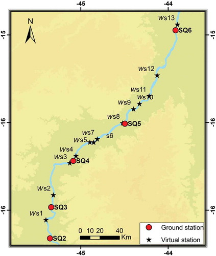
The study area is a 470-km reach of the São Francisco River in Brazil (Fig. 1). The São Francisco has an average discharge of 2850 m³/s and is a most important river for providing almost 10% of the national demand for agricultural as well as domestic and industrial water needs. A major part of its course flows through a semi-arid region further increasing its socio-economic importance (ANA 2018). Land cover near and around the section under study is divided between savanna, sclerophyllous deciduous and semi-deciduous forest, agriculture and pasture.

Figure 1. Location of the São Francisco River reach used as test area showing the in situ hydrological stations (left) and geographical context in the South American continent (right)

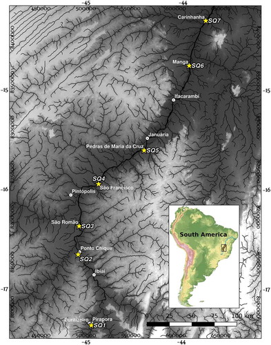
Rating curves were calculated using data from seven in situ stations from Brazil’s national water agency, Agência Nacional das Águas (ANA),² as shown in Table 2. Precise measurements of in situ discharge data (not calculated from rating curves) from ANA were used to validate and adjust the rating curves that transform water level into discharge. These adjusted discharge data were the basis for computing and validating new rating curves derived from water width data. Furthermore, the discharge was regionalized using the specific drainage area of every point along the river reach (this is more thoroughly explained in Section 3.1). Although the discharge from the in situ station database is taken here as ground truth, it is still an indirect measurement relating flow velocity measured in a number of profiles separated by some distance to construct a rating curve relating it to the water stage. Koblinsky et al. (1993) has estimated the standard error of these water stage measurements to be in the order of 0.1 m.

Table 2. Station location

Station location	ANA code	Code	S Latitude/W Longitude	Mean discharge (m^3/s)	Drainage area (km^2)	Altitude (m a.s.l.)
Pirapora	41135000	${\mathrm{S}}_{Q1}$	17°22ʹ9.12ʹ’/44°56ʹ35.2ʹ’	841	62200	480
Cachoeira da Manteiga	42210000	${\mathrm{S}}_{Q2}$	16°39ʹ 25.92ʹ’/45°4ʹ50.9ʹ’	1169	107000	467
São Romão	43200000	${\mathrm{S}}_{Q3}$	16°22ʹ21.00ʹ’/45°4ʹ12.0ʹ’	1569	154000	464
São Francisco	44200000	${\mathrm{S}}_{Q4}$	15°56ʹ57.84ʹ’/44°52ʹ4.1ʹ’	1808	184000	457
Pedras de Maria da Cruz	44290002	${\mathrm{S}}_{Q5}$	15°36ʹ3.96ʹ’/44°23ʹ48.1ʹ’	2017	194000	451
Manga	44500000	${\mathrm{S}}_{Q6}$	14°45ʹ25.92ʹ’/43°55ʹ55.9ʹ’	1953	202000	440
Carinhanha	45298000	${\mathrm{S}}_{Q7}$	14°18ʹ15.84ʹ’/43°45ʹ47.9ʹ’	2192	254000	427

A time series of river width measured at regular distance intervals along the river reach was built to serve as primary data source for creating width rating curves (wrc) from which discharge was calculated and compared with in situ data. Images from Sentinel-1 SAR (S1; 36 images), Sentinel-2 MSI (S2; 32 images) and Landsat-8 Operational Land Imager (OLI) (L8; 6 images) were used to create this width database. The time series covers the period from 1 March 2016 to 31 August 2018. Images from the S1 and S2 missions were acquired from the Copernicus Open Access Hub,³ while the L8 images came from the Earth Explorer platform.⁴ All image products included radiometric and geometric corrections. The choice of these satellite missions implies that both optical and SAR image data would be used. While optical data are frequently recognized as being easier to work with, they are often affected by unfavourable weather conditions, whereas SAR data present a much more constant and reliable response while demanding more complex processing. This also means that a rigorous approach has to be undertaken to make sure that extracting the river width from these different images (type and resolution) will generate compatible results given the importance of these measurements. We based our choices on two main studies conducted with this type of image. First, the precision of extracting a water surface from SAR data was evaluated in a series of small reservoirs to determine the most appropriate processing chain to separate water from land (Pôssa and Maillard 2018). The second study aimed at comparing all three sensors (S1, S2, L8) in a 65-km reach of the São Francisco River to test and compare the accuracy of the three different sensors for extracting the water surface (Pôssa et al. 2018). The detailed approach and results of these studies fall outside the scope of this work, but are synthesized in the Appendix. Following the conclusions of these two studies, all S1 images (36 images) were classified using the support vector machine algorithm (SVM), while the S2 (32 images) and L8 (6 images) were classified using K-means. Even though the random forest (RF) algorithm generated slightly better results, the very good performance of K-means and especially its simplicity and objectivity (no user interference apart from the number of classes; Canty 2014) made us choose the latter. The slightly lower performance with L8 was considered a minor drawback given only six L8 images were used.

Three Python3.5 programmes were created to extract the river width from the images. The three programmes are meant to be executed sequentially to produce an end-user product in the form of a shapefile and a tabulated river width data file (.csv). These programmes were planned to take advantage of satellite images (threshold of a spectral band or a classified image) to calculate the width at regular distance intervals along the river reach. The three programmes (available at Geografia Remote Sensing⁵) composing the package are:

1. SRW_River_Preparation takes a unique entry file in the form of a raster file (normally a satellite image) and prepares it for processing the centreline with the SRW_River_Centerline programme. Optionally, it can reduce the number of points of the resulting river banks shapefile.

2. SRW_River_Centerline takes the resulting binary raster from the SRW_River_Preparation and extracts a median centreline of the river by skeletonizing the raster file. This is performed only once using the image with the lowest water level to ensure the centreline is always at the same place and always in the “wet” cross-section of the river. It produces a line shapefile.

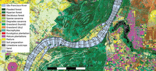
3. SRW_River_Width takes the centreline produced by SRW_River_Centerline and the river banks shapefile from the SRW_River_Preparation to calculate the river width at regular intervals. Optionally, it can use a shapefile of the islands which can then be subtracted from the river width. Figures 2 and 3 illustrate the process and results of these three programmes.

Figure 2. Steps for measuring width. Background: S1 Image; VV; acquisition 08/03/2016

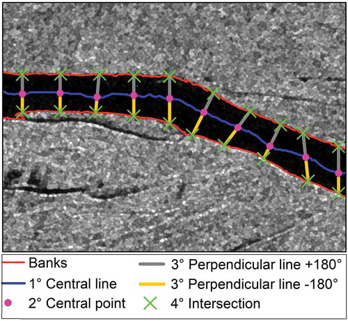
Figure 3. Illustration of the extraction of the river width from a classified image

In the case of the São Francisco River, an interval distance of 500 m was selected after a range of different intervals was tested, which showed 500 m to be a reasonable compromise to have good width differences, while preserving the significant shape changes of the river reach. Each width location can then be understood as a virtual hydrological width station (VHWS).

3.1 Regionalization of the daily mean discharge

Because there are distance lags between the discharge measured at the reference in situ stations (${\mathrm{S}}_Q$) and the VHWSs, the discharge had to be compensated for the difference in drainage area ($C{A}_{WQ/Q}$), a process called “regionalization of the discharge”. This can usually be performed using a simple compensation factor ($C{A}_{WQ/Q}$, Equation (4)(4) $C{A}_{WQ/Q}=\frac{A_{WQ}}{A_Q}$(4) ) based on the difference in area between the reference station and the VHWS. Equation (5)(5) $Q_{WQ}=Q\times C{A}_{WQ/Q}$(5) shows how the discharge at ${\mathrm{S}}_Q$ can be transferred (regionalized) to VHWSs.

(4) $C{A}_{WQ/Q}=\frac{A_{WQ}}{A_Q}$(4)

(5) $Q_{WQ}=Q\times C{A}_{WQ/Q}$(5)

where $A_{WQ}$ represents the area of contribution at the virtual station and ${\mathrm{A}}_Q$ (km²) is the contribution area at the reference station ${\mathrm{S}}_Q$ (km²), $Q$ is the discharge at the reference station ${\mathrm{S}}_Q$ (m³/s), and $Q_{WQ}$ is the transferred discharge.

As a rule-of-thumb method proposed by Euclydes et al. (2005), it was decided to apply the discharge regionalization equations (i.e. estimate the discharge based on the additional contribution area) whenever the difference between contribution areas did not exceed 30% of the reference station contribution area (Euclydes et al. 2005).

3.2 Approximating parameters a and b

Daily regionalized discharge data $Q_{WQ}$ and their respective widths were used to calibrate each virtual width station model following the power function law between these variables. The calibration of parameters $a$ and $b$ was performed using a nonlinear least square function and a k-fold cross-validation to determine the best fit model.

The k-fold technique consists in splitting the set of data into $k$ subsets. Models are trained using k – 1 subsets, and the remaining subset is used to evaluate the model generated. The process is repeated k times with a different subset composed of 80% of the original set each time, while the remaining 20% is used as a validation subset. The model generated from the subset with the best result is then chosen (James et al. 2013).

Figure 4 shows a graph schematic that illustrates the k-fold approach with the 80–20% fivefold used in this study. The number of folds ($k$) was selected so that 80% of the dates would represent at least 30 observations (Kuhn and Kjell 2013). The k-fold approach increases the chances of generating a good model without the risk of overfitting.

Figure 4. K-fold cross-validation example for k = 5. Light grey: training data, Dark grey: test data. The method first divides the data set in k subsets, then uses k – 1 subsets for training while keeping the remaining one for validation. k iterations are performed, each one testing a model build from a different fold generating a validation estimate. The mean absolute error (MAE) was used here

The mean absolute error (MAE) was used as criterion to select the best of the five models. The MAE is calculated using Equation (6)(6) $\mathrm{M}\mathrm{A}\mathrm{E}=\frac{{\sum }_{i=1}^n\left|y_i-x_i\right|}{n}$(6) and gives an unambiguous magnitude of the errors associated with the prediction set independently of the sign (+ or –) (Willmott and Matsuura 2005):

(6) $\mathrm{M}\mathrm{A}\mathrm{E}=\frac{{\sum }_{i=1}^n\left|y_i-x_i\right|}{n}$(6)

where $y_i$ is the predicted value, $x_i$ is the observed value, and $n$ is the number of samples.

3.3 Procedures for deploying virtual station

The width data set used to analyse the hydraulic geometry relationships was acquired using three different methods from which it was decided to focus on the one offering the best results. In the first method, all the width measurements ($w$) were used individually to generate virtual stations in an “at-a-station” approach (Fig. 5(a)). A total of 952 stations were generated from the satellite mosaics and for 40–75 different dates depending on the river section.

Figure 5. The three different methods of virtual (width) stations definitions: (a) individual width ($w$) at-a-station, (b) systematic average width stations ($w_n$) calculated for the whole river reach every 10 km and (c) selected average width stations ($w_s$) defined by statistically selecting river sections with the most width variations

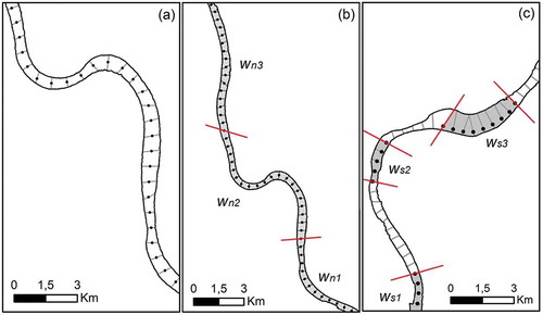
The second and third methods are based on the concept of averaging the width over a short sector (ASW or$w_e$) and was introduced by Smith et al. (1995). The ASW is calculated by averaging a number of consecutive river section widths of a given sector, which amounts to a value with the same dynamic as dividing the area of the river section by its average width ($w_n$). ASW values can then substitute $w$ in the hydraulic geometry relationship$w=\mathrm{A}\mathrm{S}\mathrm{W}=a.Q^b$ (Smith et al. 1995, Smith and Pavelsky 2008).

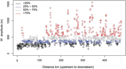
The difference between the second and third methods resides in the manner by which the river sectors are selected. The second method systematically divides the whole river reach in sectors of fixed length (10 km in our case), each of which will have its own ASW. In the third method, a statistical-spatial analysis was used to locate sectors with good potential based on the fact that the relationship between $w$ and $Q$ is influenced by the cross-section shape (Leopold and Maddock 1953). The amplitude within the time series ($w_{i\mathrm{m}\mathrm{a}\mathrm{x}}-w_{i\mathrm{m}\mathrm{i}\mathrm{n}}$) was adopted as indicator of this potential. Only the last quartile (the fourth of four), corresponding to 25% of the river cross-sections with the largest amplitude, was selected (Fig. 6). These sectors ($s_i$) were then analysed to make sure that they had a certain consistency in terms of width amplitude. Only sectors with a length equal or superior to 2 km were retained to calculate $w_s$ (Fig. 5(c)). Width data not included within the last quartile could be tolerated as long as they were isolated (bordered on each side by included values).

Figure 6. Illustration of the set of 952 river cross-sections widths organized by quartiles (25% = 55.5 m, 50% = 90.62 m, 75% = 228.86 m)

3.4 Model performance evaluation and comparison of the three methods

The performance of the models created with the three methods was evaluated with a combination of metrics: Nash-Sutcliffe model efficiency coefficient (NSE, Equation (7)(7) $\mathrm{N}\mathrm{S}\mathrm{E}=1-\left[\frac{{\sum }_{i=1}^n\left(x_i-y_i\right)2}{{\sum }_{i=1}^n\left(x_i-\bar{x}\right)2}\right]$(7) ), normalized root-mean-square error (NRMSE, Equation (8)(8) $\mathrm{N}\mathrm{R}\mathrm{M}\mathrm{S}\mathrm{E}=\frac{\sqrt{\frac{{\sum }_{i=1}^n\left(y_i-x_i\right)2}{n}}}{\bar{x}}$(8) ), percent bias (Pbias, Equation (9)(9) $\mathrm{P}\mathrm{b}\mathrm{i}\mathrm{a}\mathrm{s}=\frac{{\sum }_{i=1}^n\left(x_i-y_i\right)}{{\sum }_{i=1}^n\left(x_i\right)}\times 100$(9) ) and percentage forecast error (PFE, Equation (10)(10) $\mathrm{P}\mathrm{F}\mathrm{E}=\frac{\left(y_i-x_i\right)\times 100}{x_i}$(10) ):

(7) $\mathrm{N}\mathrm{S}\mathrm{E}=1-\left[\frac{{\sum }_{i=1}^n\left(x_i-y_i\right)2}{{\sum }_{i=1}^n\left(x_i-\bar{x}\right)2}\right]$(7)

(8) $\mathrm{N}\mathrm{R}\mathrm{M}\mathrm{S}\mathrm{E}=\frac{\sqrt{\frac{{\sum }_{i=1}^n\left(y_i-x_i\right)2}{n}}}{\bar{x}}$(8)

(9) $\mathrm{P}\mathrm{b}\mathrm{i}\mathrm{a}\mathrm{s}=\frac{{\sum }_{i=1}^n\left(x_i-y_i\right)}{{\sum }_{i=1}^n\left(x_i\right)}\times 100$(9)

(10) $\mathrm{P}\mathrm{F}\mathrm{E}=\frac{\left(y_i-x_i\right)\times 100}{x_i}$(10)

where $x_i$ represents the observed values, $y_i$ the predicted values, $\bar{x}$ the mean of the observations and $n$ the number of samples.

The NSE is used to determine the normalized magnitude of the variance of the residue by comparing it to the variance of the observed data (Nash and Sutcliffe 1970). The closer NSE gets to 1.0, the more precise the model. The NRMSE is used to support the interpretation of NSE. Pbias is used mainly to check if a trend is present in the predicted values: a positive Pbias indicates that the models tend to overestimate $Q$, whereas a negative value indicates the opposite (Moriasi et al. 2007). PFE is used to evaluate the individual errors of the predicted discharge.

4 Results and discussions

4.1 Discharge compensation

The average daily discharge from the in situ stations was regionalized to match the locations of the virtual width stations (see Section 3.1). To illustrate the validity of this procedure, Table 3 and Fig. 7 show the result of regionalizing the discharge of station SQ3 to a location 64 km downstream that corresponds to the location of SQ4 so that the result can be compared with the “true” value. Using the flood hydrograms from the two stations (SQ3 and SQ4), we estimated the lag time (∆t) of 25 h with an average flow propagation speed of 0.708 m/s, for the study period (2016–2018). The average discharge of station SQ4 was then used for comparison. An NRMSE of 8.52% was obtained for the comparison between regionalized and observed discharge. The results (QWQ in Table 3, column 4) can be compared with the actual in situ data measured at station SQ4 (Table 3, column 3).

Table 3. Transferred discharge (QWQ) of station SQ3 to a virtual station 64 km downstream that coincides with station SQ4. The PFE gives an idea of the errors generated by the approach

Dates 1–2	Station SQ3 (m^3/s)	Station SQ4 (m^3/s)	QWQ (m^3/s)	PFE QWQ – SQ4 (%)
01–02/03/2016	596.9	658.0	713.2	8.39
08–09/03/2016	909.4	1061.7	1086.5	2.34
03–04/12/2016	685.2	832.6	818.7	–1.67
15–16/12/2016	2169.6	2407.2	2592.3	7.69
13–14/02/2017	1297.0	1661.5	1549.7	–6.73
09–10/03/2017	549.9	630.7	657.1	4.18
13–14/11/2017	559.2	815.0	668.1	–18.02
10–11/12/2017	1751.3	2059.0	2092.5	1.63
28–29/12/2017	426.6	547.5	509.7	–6.90
15–16/01/2018	545.3	678.7	651.5	–4.01
20–21/02/2018	491.2	698.3	586.8	–15.97
16–17/03/2018	1715.0	1934.8	2049.1	5.91
21–22/04/2018	439.2	570.2	524.8	–7.96
07–08/05/2018	294.0	335.1	351.2	4.81
17–18/05/2018	312.3	333.2	373.1	11.96
06–07/06/2018	357.9	383.1	427.6	11.63
21–22/06/2018	338.6	348.3	404.5	16.15
16–17/07/2018	357.9	363.6	427.6	17.60
14–15/08/2018	385.6	387.0	460.7	19.05

Figure 7. Transferred discharge data (SQ QWQ) of station S_Q3 to a point 64 km downstream that coincides with station S_Q4.

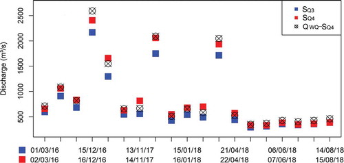
The percentage forecast error (PFE) varies between – 16 and 19, with a slight trend towards overestimation. The majority (12 out of 19) are in the interval bracket – 10% to 10%. Ouarda et al. (2018) argue that the uncertainties generated by the regionalization of the discharge are mostly attributable to other physiographical attributes of the river such as the shape of the watershed or peculiarities of the climate and its distribution. The contribution area and the geographical proximity are, therefore, not always sufficient to estimate accurately the discharge at a certain point of the river (Ouarda et al. 2001), since it neglects the dynamic component of the flow.

4.2 Comparison of the three methods

The three methods used to test the $w-Q$ relationship (individual width, w, systematic average, $w_n$, and selected average, $w_s$) were evaluated and statistically compared, and the results are presented in Figs. 8 and 9. The three methods were also compared based on the same subsection of the river reach being studied. Within this analysis, the “individual width” method yielded almost systematically worse results (except for two cases) than the other two methods, which, in turn, produced similar performances. These suggest that methods considering averages over a short river reach are more likely to generate better results. Smith et al. (1996) and Sun et al. (2010) also stress that averaging the width over a section reduces the impact of measurement errors and local variations on models relating width and discharge.

Figure 8. Model performance evaluation for virtual stations generated from the three methods

Figure 9. Evaluation metrics used to compare the results from the three discharge estimation methods: (a) individual width, $w$; (b) systematic average, $w_n$ and (c) selected average, $w_s$

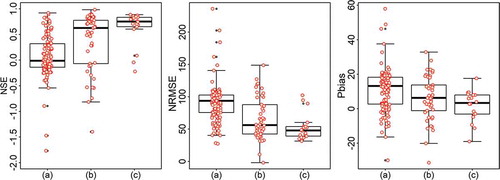
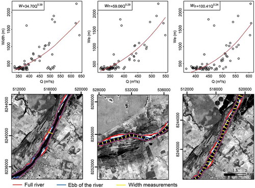
Figure 10. The best curves for the $w-Q$ relationship by method and the respective analysis sections in the river

The $w_s$ group of results was granted the largest median NSE value (NSE_med value = 0.725), followed by $w_n$ (NSE_med = 0.554) and $w$ (NSE_med = – 0.012) (Fig. 9). The same can be said about NRMSE (47.7%, 56.1% and 93.7%). It can also be observed that the difference between the two methods ($w_n$ and $w_s$) is quite small for all three metrics. It is quite clear that in the case of $w_n$, the variance is always much larger, which most likely explains the somewhat poorer results. These analyses indicate that the $w_s$ method stands out compared to the $w_n$ method because it increases performance by previously selecting potentially good areas (based on width amplitude) for observing the $w-Q$ relationship.

The Pbias values (13.20%, 7.75% and 3.35%) for the three methods show the same general trend. The fact that all three values are positive shows that the models tend to overestimate the discharge in most cases.

4.3 Estimating river discharge

The power functions and their respective evaluation metrics for the model with the best adjustment for each of the three methods are presented in Table 4 and Fig. 10. While in general terms the “individual width” method generated poorer results, it did produce the single best fit at a specific location with values of 0.92, 27.42% and 5.1% for the NSE-NRMSE-Pbias triad. The best model for the other two methods shows slightly poorer results but can be considered within the same order of magnitude for the three metrics. Although the “selected average” method gave a smaller NSE, it had the smallest Pbias of the three. In comparison, Smith et al. (1996), using the same exponential form, obtained NRMSE of between 15% and 61% using SAR images in Alaska and Canada to measure the river width. In another similar study in western Canada, Ashmore and Sauks (2006) obtained NRMSE of between 14% and 25% with orthorectified aerial photographs. Both case studies were done on braided streams in which the width varies widely with discharge.

Table 4. Best fit power functions achieved by each method

Method	Equation	NSE	NRMSE	Pbias
$w$	$Q={\left(\frac{W}{34.70}\right)}^{\frac{1}{0.39}}$	0.92	27.42	5.1
$w_n$	$Q={\left(\frac{We}{59.06}\right)}^{\frac{1}{0.29}}$	0.89	31.5	6.0
$w_s$	$Q={\left(\frac{We}{100.41}\right)}^{\frac{1}{0.24}}$	0.87	34.82	2.8

Xu et al. (2004) used an approach that combines the relationships width–stage and stage–discharge, where the width was measured from a time series of high-resolution satellite images of four trapezoidal cross-sections of the Yangtze River; they claimed an average percent accuracy of 95.2% ($Ac=100-\left[\left(yi-xi\vee xi\right)\ast 100\right]$, where $yi$ are the estimated discharge and $xi$ the measured one). For the sake of comparison, the average percent accuracies reached in this study are 85%, 61% and 70% for the three models, respectively, as shown in Table 4. We should mention that Xu et al. (2004) used images with a spatial resolution of ≈2.4 m, whereas we used S2 and L8 images of 10 and 30 m resolution, respectively.

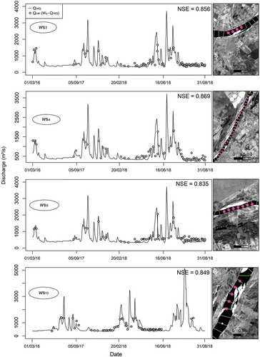
The models generated from the $w_s$ method are presented in Table 5 along with the three evaluation metrics. Figure 11 shows the location of the 13 virtual width stations. Eight of the 13 stations gave NSE values greater than 0.7.

Table 5. Models $w_s$ method. Bold values indicate best model results

Virtual station	a	b	NSE	NRMSE	Pbias
$w$s1	4.968	0.662	0.760	47.2	2.8
$w$s2	8.358	0.635	0.686	54.0	3,9
$w$s3	70.446	0.296	0.856	36.6	–3.1
$w$s4	100.417	0.243	0.869	34.8	–3.0
$w$s5	56.224	0.313	0.835	39.1	9.5
$w$s6	3.839	0.709	0.706	52.2	5.9
$w$s7	87.266	0.237	0.746	48.6	–1.6
$w$s8	129.009	0.236	0.795	43.6	2.7
$w$s9	80.714	0.297	0.605	60.2	–9.3
$w$s10	10.870	0.582	0.849	37.2	–4.8
$w$s11	0.284	1.083	–0.044	94.6	17.6
$w$s12	263.828	0.109	–0.222	102.3	–19.0
$w$s13	40.654	0.376	0.652	53.8	8.0

Figure 11. Location of the 13 virtual $w_s$ stations

Four of these virtual stations have an NSE larger than 0.8 and the time series of their estimated discharge are presented in Fig. 12. The fourth model ($w_{s4}$) presented the best fit (NSE = 0.869) and is well adjusted both in low and high discharge values. Flow duration of less than 24% (>962 m³/s) was underestimated, probably because of the scarcity of such situations in the study’s time series. Large values of PFE are associated with flow duration superior to 64% (<423 m³/s). In contrast to the study of Ashmore and Sauks (2006), who claimed larger residuals with large discharge values, our largest residuals are mostly associated with low discharge situations.

Figure 12. Daily in situ discharge (Q_obs) data (line) compared with estimated discharge calculated from the $w_s$ method for the period March 2016–August 2018

The results tend to suggest that the method can yield discharge estimates for a medium-sized river as long as the morphology of some sectors responds to an increase of discharge by widening its wet surface. Moreover, this widening should be well detectable by the imaging sensors given their spatial resolution. For the approach to work, the river should have at least a few fluviometric stations to be able to calibrate the models. In a similar approach using width data from satellite images, Gleason et al. (2014), proposed an innovative method (see Section 2) tested in 34 rivers around the world. Their method yielded mostly good result, except for three rivers, one of which was the São Francisco.

To further the analysis of the fourth model ($w_{s4}$), cross-sections were generated at six locations along this river reach. The width time series was combined with a water level time series of the nearby hydrologic station located approximately 6 km upstream to produce these partial cross-sections (Fig. 13).

Figure 13. Cross-sections at six locations along this river reach $w_{s4}$

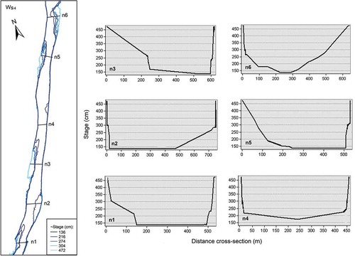
Cross-sections n2 and n4 have an almost rectangular shape that makes the relationship between discharge and width very difficult to observe. This is also partially the case for the lower portion of cross-sections n1 and n3 so that the change in discharge (hence level) will only be expressed in the width when a certain water level is attained. In the example illustrated in Fig. 13, n5, n6 and the upper portion of n1 and n3 are best suited to express the discharge variation as a function of width. The asymmetrical aspect of these four cross-sections is also a feature that has frequently been observed throughout the river reach under study. This relationship between the channel cross-section and the widening angle of the river banks is extensively discussed by Ferguson (1986).

The b exponent in the relationship $Q=a{w}^b$ has been related to the shape of the cross-section (Ferguson 1986). In our study, we were able to observe a moderate relationship between b and the width amplitude (max_w – min_w) and calculate a coefficient of correlation (Spearman) of 0.639 (Fig. 14(a)).

Figure 14. Relationships between (a) exponent $b$ and width amplitude, and (b) NRMSE and width amplitude

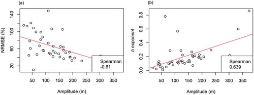
The same was observed between the width amplitude and the NRMSE, but in this case, as the amplitude increases, the NRMSE decreases (Fig. 14(b)). These relationships tend to validate the suggestion that virtual discharge stations can be based on width alone as long as a certain amount of variation is observed for a wide enough range of water levels. This also suggests that the prior selection of river sections based on the amount of width variation is a valid and desirable approach.

Furthermore, the ability to measure such width-based discharge using satellite images also depends on the spatial resolution of these images and on the revisit frequency. It is our view that the increasing number of SAR missions like Sentinel-1 and the RADARSAT Constellation Mission (RCM) will eventually provide daily image data of any place on Earth which will greatly facilitate such endeavour.

5 Conclusion

In this study, two initial methods were implemented and compared in order to determine the discharge of a medium-sized river from a time series of river width extracted from satellite images. The first method is based on individual width measurements ($w$) while the second considers the average width over a river section. The latter was then subdivided to create a third method. While it was initially considered to systematically consider all river sections of a fixed length to cover the whole river reach under study (systematic average, $w_n$), we then opted to select certain river sections of varying width based on two criteria: (i) spatial consistency and (ii) statistical appropriateness based on the analysis of the width amplitude (selected average, $w_s$).

A 470-km reach of the São Francisco River was used to implement and test the three methods. This section of the river is characterized by both near-rectangular and asymmetrical trapezoidal cross-sections Maillard (2020, in press). Our aim was to use a time series of satellite images from a variety of sensors with good spatial resolution (10–30 m) over a relatively short period (3 years) to take advantage of the recent increase in freely available systematic coverage from the recent Sentinel-1 and −2 and the Landsat-8 missions. Width-discharge models were created for non-monitored sections of the river by regionalizing the discharge based on the adjusted contribution area.

We first observe that average-based methods systematically produced better results than the “individual width” method. While both the systematic and selected average generated good results, the latter tended to show better adjustments consistently as shown by three evaluation metrics (NSE, NRMSE and Pbias). A correlation between the b exponent, taken as a cross-section shape indicator, and the width amplitude suggests that the method is especially appropriate for trapezoidal cross-section shapes which is consistent with the hydraulic geometry theory.

About 69% of the models generated with the selected average method presented NSE values better than 0.7. The evaluation of four of these models produced NSE values between 0.84 and 0.87 indicating a good fit for these types of models. It was observed that the largest residuals were associated with flow durations greater than 64% that could be the result of near-rectangular cross-sections in low waters. Conversely, high waters (larger widths) tended to overestimate the discharge. This could be caused by the reduced number of observations in high waters but also by a widening of the upper portion of the cross-sections in these conditions.

It should be stated that this kind of approach using remote sensing data to estimate hydraulic variables is not suitable for some situations. For instance, rivers margins with extensive areas of aquatic plants can produce errors in width measurements or rivers that split into numerous channels in low waters can also generate unrealistic measurements. The same goes for backwaters near coastal areas, sections of rapids and river sections with mostly rectangular cross-sections. In fact, one of the challenges involved in producing good estimates of these variables consists in choosing proper sections or reaches where these approaches are likely to generate usable measurements.

Today, the availability of in situ data from ANA’s hydrometric stations can take anything between 3 and 6 months, or even more, whereas most satellite images can be downloaded within 1 or 2 days of the sensing. Although remote sensing data will not substitute for in situ data, the facility of acquisition and processing can be combined with the method we proposed to generate rapid estimates of river discharge. Moreover, these estimates are not restricted to special locations but can be produced for any sector where the river is sufficiently wide, has width variation enabling the discharge estimation and has at least some fluviometric in situ station data to calibrate the models.

Acknowledgements

The authors are most grateful to the US National Air and Space Administration (NASA), the United States Geological Survey (USGS), the European Space Agency (ESA), Agência Nacional das Águas (ANA) and the Serviço Geológico do Brasil (CPRM) for making available the data and images necessary for the execution of this study.

Disclosure statement

No potential conflict of interest was reported by the authors.

Additional information

Funding

The authors would like to thank Coordenação de Aperfeiçoamento de Pessoal de Nível Superior (CAPES) for the postgraduate scholarship [Process no. 88882.18426712018-01] and the Universidade Federal de Minas Gerais.

Notes

¹ https://www.esa.int/Applications/Observing_the_Earth/Copernicus.

² https://www.snirh.gov.br.

³ https://scihub.copernicus.eu.

⁴ https://earthexplorer.usgs.gov.

⁵ http://www.igc.ufmg.br/.

Appendix

Water surface extraction from optical and SAR images

In order to create a time series of satellite images with minimum time gaps between dates, images from three missions involving five satellites were combined: Sentinel-1A and 1B, Sentinel-2A and 2B and Landsat-8. To make sure the results from these different image types and resolutions were compatible, two studies were performed and are reported elsewhere.

The first study was conducted in a small urban reservoir (actually a complex of three small reservoirs) known as Lake Pampulha, where a precise GNSS survey of the two smallest water bodies was done the same day as the Sentinel-1B overpass (a high resolution image was used to validate the third one). Various speckle filtering methods were applied in combination with the support vector machine (SVM) classification algorithm known for its robustness in dealing with noisy SAR image data. It was found that the Refined Lee filter used on the VV polarization produced the best results. The VV band is less prone to noise and produced better results than combined with the VH band when comparing the differences in areas and geometry with the precise survey of the reservoir banks. A high accuracy (83–85%) for two small reservoirs of less than 6 ha and very high accuracy (94.7%) for the larger one (172 ha) were obtained. These results were especially good given the small size of these water bodies where the proportion of edge/total water pixels is quite large. Figure A1 shows the SAR image and the difference maps comparing the classification with the precise delineation.

In the second study, a 65-km reach of the São Francisco River was used to test the accuracy of three different sensors: Settinel-1 C-SAR instrument, Sentinel-2 MSI sensor and Landsat-8 OLI sensor. For this study, one image of each type was processed and classified in a variety of ways to produce water surface areas that were then compared for accuracy assessment with an interpreted high-resolution Planet Scope image (spatial resolution of 3 m). All images were acquired within the same 4-day period in January 2018, with a maximum water stage difference of 10 cm (Table A1). The S-1 SAR image was calibrated (σ₀) and geometrically corrected using a digital elevation model. Because a single image was used in the case of L-8 and S-2, no radiometric correction was performed. To determine the best water extraction procedure, five supervised classification algorithms (random forest, K-nearest neighbour, maximum likelihood classification, support vector machine and Mahalanobis) and two unsupervised ones (K-means and expectation maximization cluster analysis) were tested with all band combinations of each image. On average, random forest outperformed all other methods but SVM was slightly better for the SAR data. As for the best band combination, Table A2 presents the 10 combinations for each sensor that produced the best results with the K-means algorithm (hundreds of tests were performed). Considering the results presented in Table A2, it stands out that for L-8, band 6 (SWIR) produced the best results and is present in seven of the best 10 classification results. Since for S-2, no single band produced one of the 10 better results, we chose the most recurring band within these results: Band 11 (also SWIR). Figure A2 shows a sector of the São Francisco River with the three image type results as well as the reference PlanetScope interpretation.

Figure A1. Top Sentinel-1B SAR image of the Pampulha Reservoirs complex. Bottom: difference maps between the SAR image classification results and the precise delineation. Grey pixels represent false negative errors (omitted pixels) and black pixels represent false positive errors (falsely included pixels). Reproduced with permission from the authors

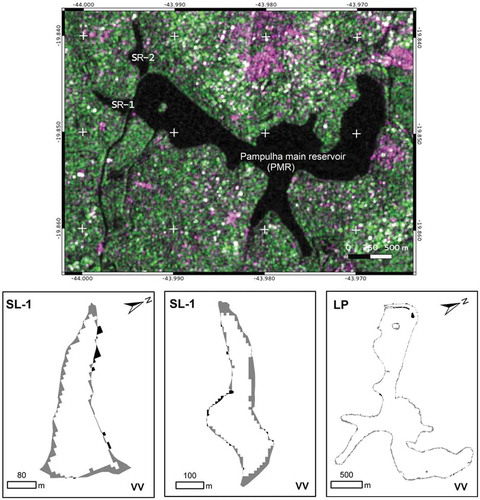
Figure A2. Left: PlanetScope false colour image. Right: water surfaces extracted from Lansat-8, Sentinel-1 and Sentinel-2 images. The background cyan colour shows the reference surface from the Planet Scope image used for determination of accuracy. Reproduced with authorization from the authors

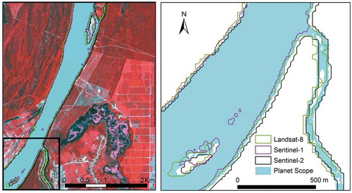
Table A1. List of images acquired with some of their specification and the associated water stage level

Sensor	Image date	Pixel size (m)	Stage (cm)*	Product level
Sentinel-1 (S-1)	15/01/18	10	223.5	Level-1GRD
Sentinel-2 (S-2)	17/01/18	10	217	1 C
PlanetScope	17/01/18	3	217	3A
Landsat/OLI (L-8)	18/01/18	30	213	L1

Table A2. Water surface classification accuracy by sensor, spectral bands and polarizations

Rank	Bands L8	Accuracy L8	Bands S-2	Accuracy S-2	Pol band S-1	Accuracy S-1
1	6	86.43	8,12	94.70	VV	93.79
2	3,6	86.22	3,8	94.48	VH	84.97
3	3,7	86.09	8A,11	94.41	VV+VH	82.00
4	6,7	85.92	8,11	94.32
5	3,6,7	85.88	6,8A,11	94.28
6	3,4,6	85.73	8,11,12	94.25
7	7	85.59	11,12	94.24
8	3,4,6,7	85.53	8A,11,12	94.21
9	3,4,7	85.46	6,8A,11,12	94.16
10	4,6,7	85.28	6,11,12	94.13

References

- Alsdorf, D.E., Rodríguez, E., and Lettenmaier, D.P., 2007. Measuring surface water from space. Reviews of Geophysics, 45 (2). doi:10.1029/2006RG000197
- ANA, 2018. São Francisco [online]. Available from: http://www3.ana.gov.br/portal/ANA/sala-de-situacao/sao-francisco. [Accessed 9 May 2018].
- Ashmore, P. and Sauks, E., 2006. Prediction of discharge from water surface width in a braided river with implications for at a station hydraulic geometry. Water Resources Research, 42 (3), 2006. doi:10.1029/2005WR003993
- Canty, M.J., 2014. Image analysis, classification and change detection in remote sensing: with algorithms for ENVI/IDL and Python. Boca Raton, FL: CRC Press.
- Chu, Z.X., et al., 2006. Changing pattern of accretion/erosion of the modern Yellow River (Huanghe) subaerial delta, China: based on remote sensing images. Marine Geology, 227 (1–2), 13–30. doi:10.1016/j.margeo.2005.11.013
- de Oliveira, L.M., Maillard, P., and de Andrade Pinto, E.J., 2017. Application of a land cover pollution index to model non-point pollution sources in a Brazilian watershed. Catena, 150, 124–132. doi:10.1016/j.catena.2016.11.015
- Elmi, O., Tourian, M.J., and Sneeuw, N., 2015. River discharge estimation using channel width from satellite imagery. In: 2015 IEEE International Geoscience and Remote Sensing Symposium (IGARSS). Milan: IEEE, 727–730.
- ESA (European Space Agency), 2018. Sentinel-1 - the SAR imaging constellation for land and ocean services [online]. Available from: https://directory.eoportal.org/web/eoportal/satellite-missions/c-missions/copernicus-sentinel-1. [Accessed 9 May 2018].
- Euclydes, H.P., Ferreira, P.A., and Filho, R.F.F., 2005. Atlas digital das águas de Minas: uma ferramenta para o planejamento e gestão dos recursos hídricos. [CD-ROM]. Belo Horizonte: Ruralminas/UFV.
- Ferguson, R.I., 1986. River loads underestimated by rating curves. Water Resources Research, 22 (1), 74–76. doi:10.1029/WR022i001p00074
- Frappart, F., et al., 2005. Floodplain water storage in the Negro River basin estimated from microwave remote sensing of inundation area and water levels. Remote Sensing of Environment, 99 (4), 387–399. doi:10.1016/j.rse.2005.08.016
- Fryirs, K.A. and Brierley, G.J., 2012. Geomorphic analysis of river systems: an approach to reading the landscape. Hoboken: John Wiley & Sons.
- Gleason, C.J. and Smith, L.C., 2014. Toward global mapping of river discharge using satellite images and at-many-stations hydraulic geometry. Proceedings of the National Academy of Sciences, 111 (13), 4788–4791. doi:10.1073/pnas.1317606111
- Gleason, C.J., Smith, L.C., and Lee, J., 2014. Retrieval of river discharge solely from satellite imagery and at-many-stations hydraulic geometry: sensitivity to river form and optimization parameters. Water Resources Research, 50 (12), 9604–9619. doi:10.1002/2014WR016109
- Gleason, C.J. and Wang, J., 2015. Theoretical basis for at many stations hydraulic geometry. Geophysical Research Letters, 42 (17), 7107–7114. doi:10.1002/2015GL064935
- Haas, E.M., Bartholomé, E., and Combal, B., 2009. Time series analysis of optical remote sensing data for the mapping of temporary surface water bodies in sub-Saharan western Africa. Journal of Hydrology, 370 (1–4), 52–63. doi:10.1016/j.jhydrol.2009.02.052
- James, G., et al., 2013. An introduction to statistical learning. New York: Springer.
- Jensen, J.R., 2006. Remote sensing of the environment: an earth resource perspective. Upper Saddle River, NJ: Prentice Hall.
- Kim, D., et al., 2019. Ensemble learning regression for estimating river discharges using satellite altimetry data: Central Congo River as a Test-bed. Remote Sensing of Environment, 221, 741–755. doi:10.1016/j.rse.2018.12.010
- Knighton, A.D., 1974. Variation in width-discharge relation and some implications for hydraulic geometry. Geological Society of America Bulletin, 85 (7), 1069–1076. doi:10.1130/0016-7606(1974)85<1069:VIWRAS>2.0.CO;2
- Koblinsky, C., et al., 1993. Measurements of river level variations with satellite altimetry. Water Resources Research, 29 (6), 1839–1848. doi:10.1029/93WR00542
- Kuhn, M. and Kjell, J., 2013. Applied predictive modeling. New York: Springer.
- Leopold, L.B. and Maddock, T., 1953. The hydraulic geometry of stream channels and some physiographic implications. Washington, DC: US Government Printing Office, 253.
- Maillard, P., 2020 (in press). Using time series of Sentinel-1 images to produce dry bathymetry of rivers. ISPRS Annals of the Photogrammetry, Remote Sensing and Spatial Information Sciences, V-3-2020, 387–394. doi:10.5194/isprs-annals-V-3-2020-387-2020.
- Moriasi, D.N., et al., 2007. Model evaluation guidelines for systematic quantification of accuracy in watershed simulations. Transactions of the ASABE, 50 (3), 885–900. doi:10.13031/2013.23153
- Mueller, N., et al., 2016. Water observations from space: mapping surface water from 25 years of Landsat imagery across Australia. Remote Sensing of Environment, 174, 341–352. doi:10.1016/j.rse.2015.11.003
- Nace, R.L., 1964. The international hydrological decade. Eos, Transactions American Geophysical Union, 45 (3), 413–421. doi:10.1029/TR045i003p00413
- Nash, J.E. and Sutcliffe, J.V., 1970. River flow forecasting through conceptual models part I - A discussion of principles. Journal of Hydrology, 10 (3), 282–290. doi:10.1016/0022-1694(70)90255-6
- Ouarda, T., et al., 2001. Regional flood frequency estimation with canonical correlation analysis. Journal of Hydrology, 254 (1–4), 157–173. doi:10.1016/S0022-1694(01)00488-7
- Ouarda, T., et al., 2018. Introduction of the GAM model for regional low-flow frequency analysis at ungauged basins and comparison with commonly used approaches. Environmental Modelling & Software, 109, 256–271. doi:10.1016/j.envsoft.2018.08.031
- Pavelsky, T.M., et al., 2014. Assessing the potential global extent of SWOT river discharge observations. Journal of Hydrology, 519, 1516–1525. doi:10.1016/j.jhydrol.2014.08.044
- Pekel, J.F., et al., 2016. High-resolution mapping of global surface water and its long-term changes. Nature, 540 (7633), 418–422. doi:10.1038/nature20584
- Pôssa, É.M., et al., 2018. On water surface delineation in rivers using Landsat-8, Sentinel-1 and Sentinel-2 data. In: Proc. SPIE 10783. Remote Sensing for Agriculture, Ecosystems, and Hydrology XX. Berlin: International Society for Optics and Photonics.
- Pôssa, É.M. and Maillard, P., 2018. Precise delineation of small water bodies from sentinel-1 data using support vector machine classification. Canadian Journal of Remote Sensing, 44 (3), 179–190. doi:10.1080/07038992.2018.1478723
- Shiklomanov, I.A., 1993. World freshwater resources. In: P.H. Gleick, ed. Water in crisis: a guide to the world’s fresh water resources. Oxford, UK: Oxford University Press, 13–24.
- Sichangi, A., Wang, L., and Hu, Z., 2018. Estimation of river discharge solely from remote-sensing derived data: an initial study over the Yangtze river. Remote Sensing, 10 (9), 1385. doi:10.3390/rs10091385
- Singh, V.P. and Zhang, L., 2008. At-a-station hydraulic geometry relations, 1: theoretical development. Hydrological Processes: An International Journal, 22 (2), 189–215. doi:10.1002/hyp.6411
- Smith, L.C., et al., 1995. Estimation of discharge from braided glacial rivers using ERS 1 synthetic aperture radar: first results. Water Resources Research, 31 (5), 1325–1329. doi:10.1029/95WR00145
- Smith, L.C., et al., 1996. Estimation of discharge from braid rivers using synthetic apertureradar imagery: potential application to ungauged basins. Water Resources Research, 32 (7), 2021–2034. doi:10.1029/96WR00752
- Smith, L.C. and Pavelsky, T.M., 2008. Estimation of river discharge, propagation speed, and hydraulic geometry from space: Lena River, Siberia. Water Resources Research, 44 (3). doi:10.1029/2007WR006133
- Sun, W.C., Ishidaira, H., and Bastola, S., 2010. Towards improving river discharge estimation in ungauged basins: calibration of rainfall-runoff models based on satellite observations of river flow width at basin outlet. Hydrology and Earth System Sciences, 14 (10), 2011–2022. doi:10.5194/hess-14-2011-2010
- Tang, Q., et al., 2009. Remote sensing: hydrology. Progress in Physical Geography, 33 (4), 490–509. doi:10.1177/0309133309346650
- Tarpanelli, A., et al., 2013. Toward the estimation of river discharge variations using MODIS data in ungauged basins. Remote Sensing of Environment, 136, 47–55. doi:10.1016/j.rse.2013.04.010
- Tarpanelli, A., et al., 2019. Daily river discharge estimates by merging satellite optical sensors and radar altimetry through artificial neural network. IEEE Transactions on Geoscience and Remote Sensing, 57 (1), 329–341. doi:10.1109/TGRS.2018.2854625
- The Ad Hoc Committee Group, et al., 2001. Global water data: a newly endangered species. EOS Transactions. American Geophysical Union, 82 (5), 54–58. doi:10.1029/01EO00031
- Tourian, M.J., et al., 2016. Spatiotemporal densification of river water level time series by multimission satellite altimetry. Water Resources Research, 52 (2), 1140–1159. doi:10.1002/2015WR017654
- Villar, R.E., et al., 2013. A study of sediment transport in the Madeira River, Brazil, using MODIS remote-sensing images. Journal of South American Earth Sciences, 44, 45–54. doi:10.1016/j.jsames.2012.11.006
- Wass, P.D., et al., 1997. Monitoring and preliminary interpretation of in-river turbidity and remote sensed imagery for suspended sediment transport studies in the Humber catchment. Science of the Total Environment, 194, 263–283. doi:10.1016/S0048-9697(96)05370-3
- Willmott, C.J. and Matsuura, K., 2005. Advantages of the mean absolute error (MAE) over the root mean square error (RMSE) in assessing average model performance. Climate Research, 30 (1), 79–82. doi:10.3354/cr030079
- Xu, K., et al., 2004. Estimating river discharge from very high‐resolution satellite data: a case study in the Yangtze River, China. Hydrological Processes, 18 (10), 1927–1939. doi:10.1002/hyp.1458
- Zhang, J., et al., 2004. Estimation of river discharge from non-trapezoidal open channel using QuickBird-2 satellite imagery. Hydrological Sciences Journal, 49 (2). doi:10.1623/hysj.49.2.247.34831