Multi-site statistical downscaling of precipitation using generalized hierarchical linear models: a case study of the imperilled Lake Urmia basin

ABSTRACT

A downscaling model capable of explaining the temporal and spatial variability of regional hydroclimatic variables is essential for reliable climate change studies and impact assessments. This study proposes a novel statistical approach based on generalized hierarchical linear model (GHLM) to downscale precipitation from the outputs of general circulation models (GCMs) at multiple sites. GHLM partitions the total variance of precipitation into within- and between-site variability allowing for transferring information between sites to develop a regional downscaling model. The methodology is demonstrated by downscaling precipitation using the outputs of eight GCMs in Lake Urmia basin in northwestern Iran. Multi-model ensemble simulations are merged and bias-corrected using Bayesian model averaging and equidistant quantile mapping, respectively. The results of this study show projected declining trends in precipitation resulting in approximately 11.2% and 15.3% decrease during 2060–2080 compared to the historical period of 1985–2005 considering representative concentration pathways (RCPs) 4.5 and 8.5, respectively.

KEYWORDS:

• climate change impact
• downscaling
• precipitation
• hierarchical linear model
• Bayesian model averaging
• Lake Urmia

Editor A. Fiori Associate editor A. Requena

1 Introduction

General circulation models (GCMs) are commonly used to assess the impacts of climate change on hydroclimate variables. However, due to their coarse resolution, an intermediate model, i.e. downscaling model, is required to map their outputs to local variables. Dynamical downscaling through regional climate models (RCMs) can represent the physical dynamics of regions of interest and preserve the spatial correlations and physical relationships between multiple variables. As RCMs are computationally intensive, there is still great demand and interest in the development and application of robust statistical downscaling methods.

1.1 Statistical downscaling

Statistical downscaling provides a low-cost and rapid assessment of regional climate change impacts through the development of an empirical relationship between GCM outputs and hydroclimatic variables at catchment- or station-scales. The empirical relationship involves a deterministic or probabilistic mathematical model to represent linear or nonlinear relationships between large-scale atmospheric variables and local-scale hydroclimatic components (Nasseri et al. 2013). Commonly applied methods include multiple linear regression (MLR; e.g. Loukas et al. 2008), generalized linear model (GLM; e.g. Liu et al. 2012), artificial neural network (e.g. Samadi et al. 2012), least square support vector machine (e.g. Sachindra et al. 2013), and hybrid methods (e.g. Das and Umamahesh 2016, Lin et al. 2016).

1.1.1 Multiple linear regression (MLR)

Among the mentioned methods, MLR has gained considerable attention because of its relative simplicity, effectiveness, and probabilistic nature, which allows for the generation of a large number of samples to characterize some aspects of climate uncertainty such as natural variability (Wilby et al. 2004). The model can take nonlinear transformations of large-scale variables as new predictors while maintaining the linearity in model parameters (Wilks 2011). Statistical DownScaling model (SDSM) is an MLR-based downscaling package developed by Wilby et al. (2002), which is designed to project future daily time series under climate change at single sites.

In spite of the wide application of MLR to single-site downscaling, the model has strong limitations in multi-site downscaling because it does not characterize the significant cross correlations that exist between hydroclimatic variables recorded in different sites. Neighbouring sites are usually governed by the same large-scale atmospheric and oceanic processes; hence, hydroclimatic variables at these sites do not behave independently, but rather covary (Wilks 2011). This covariability needs to be addressed in a multi-site downscaling procedure by linking stations together. While some studies have developed separate models for each site individually neglecting the relationships among sites (e.g. Goly et al. 2014, Okkan and Kirdemir 2016, Pang et al. 2017), some others have attempted to construct a single representative time-series of the hydroclimatic variable of interest over the study region, followed by employing a conditional resampling technique to disaggregate the representative series to constituent sites (e.g. Harpham and Wilby 2005, Kannan and Ghosh 2013).

1.1.2 Weather generators

Weather generators play a pivotal role in statistical downscaling. Single-site weather generation is a process in which random weather sequences are generated such that the statistical properties of the generated sequences resemble those of historical observations at a particular site. The general idea behind modelling single-site daily precipitation involves a two-step procedure. In the first step, precipitation occurrence process is modelled to identify wet and dry days. In the second step, the distribution of precipitation amounts in wet days is represented (Woolhiser 1992). A review of single-site weather-generation techniques is presented by Mehrotra et al. (2006). Some weather generators including LARS-WG (Long Ashton Research Station Weather Generator; Semenov and Barrow 1997), AAFC-WG (Agriculture and Agri-Food Canada Weather Generator; Hayhoe 2000), and PRECIS (Providing Regional Climates for Impacts Studies; Jones et al. 2004) are specifically used to downscale GCM outputs at single sites for climate change impact studies.

Space-time weather generators, which are the extensions of single-site weather generators, aim to represent cross correlation among neighbouring sites besides preserving statistical properties at each site. Multi-site weather generators can be classified into parametric (e.g. Bardossy and Plate 1992, Wilks 1998, Qian et al. 2002, Baigorria and Jones 2010) and non-parametric (e.g. Rajagopalan and Lall 1999, Harrold et al. 2003, Mehrotra and Sharma 2006, Sharif and Burn 2007, Lee et al. 2012) methods. Parametric weather generators attempt to represent some important physical aspects of precipitation generation mechanism through a large set of parameters. As model calibration and validation require significant efforts, particularly with a large number of sites, the operational applications of parametric weather generators are limited (Mehrotra et al. 2006). Non-parametric weather generators do not presume a joint probability distribution among weather variables and sites. This feature gives them the ability to model complex dependence structures in the observations of variables (Mehrotra et al. 2006, Verdin et al. 2018). The non-parametric nature of this type of weather generators, however, limits their application to out-of-sample data in both space and time (Verdin et al. 2019).

1.1.3 Generalized linear model (GLM)

The generalized linear model (GLM) has gained considerable attention as a comparatively simple stochastic technique to model and downscale weather variables (e.g. Stern and Coe 1984, Furrer and Katz 2007, Kim et al. 2012). A practical advantage of GLM is that it can effectively handle discrete variables such as precipitation occurrence as well as non-normally distributed variables such as precipitation amount. Furthermore, GLMs can include a set of relevant covariates in the simulation of weather variables. This allows for downscaling the outputs of GCMs to weather variables at any site. For instance, GLIMCLIM (Generalised LInear Modelling of daily CLIMate sequences; Chandler 2002) is a statistical downscaling model founded on GLMs that is used to generate daily weather sequences under climate change (e.g. Beecham et al. 2014, Rashid et al. 2015, Fu et al. 2018). Recently, there have been growing efforts to develop space-time weather generators based on GLMs which can incorporate large-scale climate variables to generate weather sequences at any arbitrary location and spatial resolution (Kleiber et al. 2012, 2013, Verdin et al. 2015, 2018, 2019).

1.2 Generalized hierarchical linear model (GHLM)

This study proposes a multi-site downscaling framework using the GHLM, which is the extension of GLM that partitions the total variance of a predictand into different sources of variability. Hence, it can handle grouped data in which a predictand varies within- and between-groups. Owing to this property, the proposed methodology offers three contributions to multi-site downscaling. First, GHLM can convey information between stations so that it can establish a more reliable link between large-scale atmospheric predictors and station-scale precipitation. This would address one of the limitations of statistical downscaling techniques, i.e. requiring sufficiently long observations, particularly in regions with limited records. Second, GHLM can explain both within- and between-station variability; hence, the downscaling model can provide a better understanding of precipitation variability over the study area. Third, the proposed framework can be viewed as a regional downscaling model in that it allows for downscaling precipitation at ungauged locations.

The hierarchical linear model (HLM) is a special case of GHLM that can model normally distributed variables. HLM, also called multilevel model, linear mixed model, and random effects model, has been used in a wide range of scientific disciplines (Raudenbush and Bryk 2002). In hydrology, Clarke (2001) used HLM for annual flood regionalization and record augmentation. He showed that HLM can provide reliable estimates of the mean annual floods at sites with short records by combining data from each site with the ones from the neighbouring sites. Booker and Dunbar (2008) used HLM to build discharge–hydraulic geometry relationship for 3600 measuring stations in England and Wales. They estimated the width, mean depth, and mean velocity of the flow at ungauged sites by grouping data into stations, stations into rivers, and rivers into hydrologic regions. Lessels and Bishop (2013) proposed HLM to predict total phosphorus and total nitrogen and their spatial autocorrelation using observed turbidity and discharge at the outlets of two catchments in southeast Australia. Slaets et al. (2014) developed HLMs to predict concentrations of suspended sediment, particulate organic carbon, and particulate nitrogen from turbidity, discharge, and rainfall at four sites in a catchment in northwest Vietnam. In their study, HLMs outperformed MLRs as they accounted for the serial correlations of the observations. Hanel and Buishand (2015) showed the application of HLM to quantifying the contribution of three sources of uncertainty, including natural climate variability, climate model structure, and future greenhouse gas emission scenarios in GCM simulated precipitation anomalies. Kamruzzaman et al. (2016) analysed the trends and the intensity–duration relationship of the maximum monthly rainfall at six stations in southern Australia. They showed that HLM can effectively handle data with unequal record lengths at multiple sites.

1.3 Lake Urmia basin

The methodology proposed in this study is applied to Lake Urmia basin, which is a hydrologically critical region attracting international attention. Lake Urmia, in the northwest of Iran, was the sixth-largest salt lake on Earth at its original extent. In recent decades, the lake level has been declining at an alarming rate raising questions about its survival in the future. While anthropogenic climate change is blamed as one of the main contributors to this trend, besides water mismanagement, it is still not clear to what extent climate change plays a role. Alizadeh-Choobari et al. (2016) estimated that evaporation from Lake Urmia has risen by 6.2 mm per decade due to the increase in temperature at a rate of 0.18°C per decade. In addition, precipitation has declined by 9.0 mm per decade over Lake Urmia basin. On the other hand, agricultural land areas have been expanded rapidly such that water demand has surpassed water supply. Hence, both meteorological and socio-economic droughts have contributed to the shrinkage of the lake. Hydrological modelling by Shadkam et al. (2016) suggests that runoff ending up in the Lake Urmia has dropped by 48% during 1960–2010. Three-third of this decline is associated with climatic changes, and two-third of that is attached to water resources development. Chaudhari et al. (2018) conducted two simulations using hydrological modelling, one with and another without anthropogenic activities, during 1995–2010. Results showed that human activities are responsible for 1.74 km³/year reduction in inflow to Lake Urmia causing about 86% decline in the lake’s volume. The study concludes that mismanagement of Lake Urmia basin is a key factor in the depletion of the lake besides prolonged droughts. Khazaei et al. (2019) believe that climate change is not a primary driver of Lake Urmia desiccation based on an analysis which showed that changes in precipitation, temperature, and soil moisture cannot explain the sharp decline of the lake’s water level since 2000. Developing of agricultural lands, on the other hand, exhibits a significant correlation with the lake’s level due to massive water consumption and diversion upstream of the lake. These studies imply that there is still large room for examining how much climate change is involved in Lake Urmia crisis. This study provides critical information about future precipitation changes over this region, which can support the development of more robust mitigation plans.

In this paper, predictor selection, downscaling procedure based on HLMs and GHLMs, and model validation are described in Section 2. The application of the proposed approach is demonstrated through a case study described in Section 3, followed by the summary and concluding remarks in Section 4.

2 Methodology

2.1 Predictor selection

Downscaling predictors that are likely to affect the predictand are called probable predictors (Sachindra and Perera 2016). Since including all these predictors in a downscaling model may cause overfitting, a promising set of variables, called potential predictors, need to be selected (Wilby et al. 2004, Wilks 2011, Sachindra and Perera 2016). The relationship between the selected predictors and the predictand is expected to be physically meaningful, statistically significant, and realistically represented by GCMs (Wilby et al. 2004). Correlation analysis is widely used to select potential predictors. In this approach, correlations between all predictors and a predictand are calculated, and predictors having the largest values are selected. Then significant cross-correlations among selected predictors can be detected using partial correlation analysis to avoid multicollinearity (Wilby and Harris 2006).

2.2 Description of the GHLM

Neglecting the nested structure of the dataset, as in GLM, would result in complete-pooling (or aggregation) bias, misestimated standard errors, and heterogeneity of the model. GHLM is the extension of GLM where the intercept and slope coefficients can be different for each group of the nested data. In these models, the variance of the regression model is partitioned into the individual variability of the error terms at each stage of the hierarchy. Contrary to the widely used GLM approach, these models are not bound by the assumption of independence between groups of observations (Raudenbush and Bryk 2002).

To explain GHLM effectively, we elaborate on HLM as a special case of GHLM that allows for modelling normally distributed variables. Then we readily expand HLM to GHLM. Consider the simple model $y_i=\alpha +\beta x_i+{ϵ}_i$, ${ϵ}_i\sim N\left(0,{\sigma }^2\right)$, $i=1,\dots ,T$, where $x$ is a large-scale climate predictor, $y$ is the predictand (i.e. precipitation), $\alpha$ is the intercept, $\beta$ is the slope, $ϵ$ is the error, and $T$ represents the number of observations. This model can be generalized to the so-called varying-intercept model when $T$ observations are clustered into $S$ groups: $y_i={\alpha }_{j\left[i\right]}+\beta x_i+{ϵ}_i$, ${ϵ}_i\sim N\left(0,{\sigma }^2\right)$, $i=1,\dots ,T$, and $j=1,\dots ,S$, where the intercept varies by each group while the slope is the same for all. The notation ${\alpha }_{j\left[i\right]}$ denotes the intercept for the $j$th group containing the $i$th observation. This can be further extended to a varying-intercept and -slope model: $y_i={\alpha }_{j\left[i\right]}+{\beta }_{j\left[i\right]}{x}_i+{ϵ}_i$, ${ϵ}_i\sim N\left(0,{\sigma }^2\right)$, $i=1,\dots ,T$, where both intercept and slope would vary by each group. This equation represents the data-level model of HLM.

In HLM, the parameters of the data-level model are described through a group-level regression model. Considering the varying-intercept model $y_i={\alpha }_{j\left[i\right]}+\beta x_i+{ϵ}_i$, the group-level regression for ${\alpha }_j$ can be described by ${\alpha }_j={\gamma }_0+{\gamma }_1{z}_j+{\eta }_j^{\alpha }$, ${\eta }_j^{\alpha }\sim N\left(0,{\tau }^2\right)$, $j=1,\dots ,S.$ ${\gamma }_0$ and ${\gamma }_1$ are the intercept and slope of the group-level model, respectively, $z$ is the predictor, and ${\tau }^2$ is the variance of the error term ${\eta }_j^{\alpha }$. While $x$ is a data-level predictor that explains the within-group variability of the predictand (i.e. the variation of precipitation within each station) $z$ is a group level predictor which describes between-group variability (i.e. the variation of precipitation between stations). Data- and group-level parameters are estimated simultaneously.

When groups are highly correlated, a large portion of the between-group variability can be explained by $z$, and the error variance of the group-level model ${\tau }^2$ would approach zero. It suggests that a single regression model can represent data from all groups, which are closely interconnected (i.e. complete-pooling). Conversely, when correlation is low, $z$ cannot account for between-group variability, and ${\tau }^2$ would take larger values as the errors of the group-level model increase. It suggests that a separate regression model is required for each group since they are independent from each other (i.e. no-pooling). While HLMs represent the partial-pooling approach, they also perform well for these two scenarios (Gelman and Hill 2007).

GHLM is the extension of HLM that relates a linear combination of a set of predictors to the mean of a predictand using a link function such that:

(1) $\begin{array}{r}\begin{array}{ccc}& g\left({\mu }_i\right)={\beta }_{j\left[i\right]}^0+{\beta }_{j\left[i\right]}^1{x}_i^1+\cdots +{\beta }_{j\left[i\right]}^k{x}_i^k,& i=1,\cdots ,T,\\ & j=1,\cdots ,S\end{array}\end{array}$(1)

where ${\mu }_i$ is the mean of ith observation of the predictand, $g(\cdot )$ is the link function, ${\beta }_{j\left[i\right]}^k$ is the kth coefficient of the jth group that contains the ith observation, and $x_i^k$ is the ith value of the kth predictor corresponding to the ith observation of the predictand. Given that precipitation amount is commonly represented by the gamma distribution (Wilks 2011), the link function of a GHLM whose predictand follows the gamma distribution is the reciprocal function:

(2) $\begin{array}{r}\begin{array}{ccc}& g\left({\mu }_i\right)=\frac{1}{{\mu }_i}={\beta }_{j\left[i\right]}^0+{\beta }_{j\left[i\right]}^1{x}_i^1+\cdots +{\beta }_{j\left[i\right]}^k{x}_i^k,& i=1,\cdots ,T,\\ & j=1,\cdots ,S.\end{array}\end{array}$(2)

Assuming that precipitation occurrence consists of Bernoulli trials, logistic HLM, which is a special case of GHLM, can be used to model precipitation occurrence. A logistic HLM relates a linear combination of a set of relevant predictors to the probability of precipitation occurrence via the logistic link function:

(3) $\begin{array}{r}\begin{array}{ccc}& \mathrm{l}\mathrm{n}\left(\frac{o_i}{1-o_i}\right)={\beta }_{j\left[i\right]}^0+{\beta }_{j\left[i\right]}^1{x}_i^1+\cdots +{\beta }_{j\left[i\right]}^k{x}_i^k,& i=1,\cdots ,T,\\ & j=1,\cdots ,S\end{array}\end{array}$(3)

where $o_i$ is the probability of precipitation occurrence corresponding to the ith observation.

The Akaike Information Criterion (AIC; Akaike 1974), as the measure of a model’s out-of-sample predictive skill, is used in a step-wise approach to identify the optimum GHLM structure. It is calculated based on $\mathrm{A}\mathrm{I}\mathrm{C}=-2\mathrm{l}\mathrm{o}\mathrm{g}\left(\mathrm{l}\mathrm{i}\mathrm{k}\mathrm{e}\mathrm{l}\mathrm{i}\mathrm{h}\mathrm{o}\mathrm{o}\mathrm{d}\right)+2p$, where $p$ represents the number of parameters in the model. The GHLM structure with the lowest AIC is selected for downscaling the outputs of GCMs.

In this study, the lme4 package in the R programming language (Bates et al. 2015) is used to estimate the parameters of GHLMs. The textbook by Gelman and Hill (2007) is an excellent reference for GHLMs, which also details the implementation of the lme4 package.

2.3 Model performance evaluation

The performance of the proposed methodology is evaluated from two different perspectives. From regionalization viewpoint, the ability of GHLM to downscale precipitation at sites that are not involved in model calibration is examined through leave-one-station-out cross-validation. From the second point of view, the improved ability of GHLM in downscaling precipitation with respect to GLM, which does not take between-station correlations into account, is evaluated using k-fold cross-validation.

Leave-one-station-out cross-validation is applied using the following algorithm:

1. Given $S$ sites, select $\left(S-1\right)$ sites for calibration and leave one site out for validation.

2. Fit GHLM to the $\left(S-1\right)$ calibration sites.

3. Downscale precipitation at the validation sites, which does not contribute to the estimation of the parameters, using the calibrated GHLM.

4. Repeat steps 1 to 3 so that each site is selected for validation once.

5. Calculate the Nash-Sutcliffe efficiency coefficient ($C_{\mathrm{N}\mathrm{S}\mathrm{E}}$; Nash and Sutcliffe 1970) and the Spearman’s correlation coefficient ($\rho$) between the downscaled and observed values to quantify the performance of GHLM in regionalization.

The k-fold cross-validation is implemented through the following algorithm:

1. Divide the historical data into $k$ sets.

2. 2. Select one particular site.

3. For all stations, assign the data in $\left(k-1\right)$ sets to calibration and the data in one set to validation.

4. Fit GLM to the calibration data of the selected site in Step 2, and use the calibrated GLM to downscale precipitation for the validation data of the selected site.

5. Fit GHLM to the calibration data of all sites as GHLM is proposed as a multi-site downscaling model, and use the calibrated model to downscale precipitation for the validation data of the selected site in Step 2.

6. Repeat steps 3 to 5 $k$ times so that each data point of the selected site in Step 2 participates once in validation.

7. Repeat steps 2 to 6 so that all sites are selected once.

8. Calculate $C_{\mathrm{N}\mathrm{S}\mathrm{E}}$ and $\rho$ between the downscaled and observed values to compare the out-of-sample performance of GLM and GHLM.

2.4 Multi-model ensemble averaging

It is now widely recognized that multi-model ensemble means provide more reliable predictions compared to the individual models (Weigel et al. 2008, Najafi and Moradkhani 2016). In weighted averaging techniques, each ensemble member is weighted according to its performance relative to observations over the historical period. Bayesian model averaging (BMA; Hoeting et al. 1999) is such an approach that has shown satisfactory results in previous studies (e.g. Raftery et al. 2005, Duan et al. 2007, Liang et al. 2013). In this study, BMA is used to combine the ensemble members of downscaled precipitation from the outputs of multiple GCMs through the development of a predictive probability density function (pdf) that is obtained from the weighted average of single model pdfs.

According to the law of total probability, the BMA predictive pdf of a quantity of interest, $p(y|D)$, is given by:

(4) $p\left(y|D\right)=\sum _{k=1}^{K}p\left(M_k|D\right)\cdot p_k\left(y|M_k,D\right)$(4)

where $p_k(y|M_k,D)$ is the posterior pdf of $y$ based on the model $M_k$ and observed dataset $D$, and $p(M_k|D)$ is the posterior pdf of model $M_k$ being correct given $D$. $p(M_k|D)$ represents the performance of model $M_k$ and shows the corresponding BMA weight of that model, i.e. $w_k=p\left(M_k|D\right)$, and $\sum _{k=1}^K{w}_k=1$.

The mean of BMA predictions is expressed as:

(5) $E\left(y|D\right)=\sum _{k=1}^{K}p\left(M_k|D\right)\cdot E\left[p_k\left(y|M_k,D\right)\right]=\sum _{k=1}^K{w}_k{\mu }_k$(5)

where ${\mu }_k$ is the mean of the predictand $y$ given the model $M_k$ and observation $D$. The BMA mean of the predictand $y$, $E(y|D)$, is the weighted average of the individual model means. The weights are inferred using the expectation–maximization algorithm (Dempster et al. 1977). BMA assumes that the predictand follows a Gaussian distribution. In the case of precipitation, which is a skewed variable, transformation methods such as Box-Cox can be applied such that the predictand approximately follows a Gaussian distribution (Raftery et al. 2005). The readers are referred to Raftery et al. (2005) and Duan et al. (2007) for the details of BMA and the EM algorithm.

2.5 Bias-correction using equidistant quantile mapping (EQM)

GCM outputs commonly show systematic errors (biases) due to the limited understanding and simplified representation of climate system processes, coarse spatial resolution, and numerical and parameterization schemes (Nahar et al. 2017). Bias-correction aims to isolate climate change signals from systematic errors (Maurer and Pierce 2014), which can be applied to the GCM outputs or downscaled variables at the local scale. The equidistant quantile mapping (EQM) method introduced by Li et al. (2010) is a modified version of quantile mapping technique, which has shown good performance in previous studies (e.g. Srivastav et al. 2014, Sachindra et al. 2014a, Mehrotra and Sharma 2016, Okkan and Kirdemir 2016). The first step in EQM is to derive the empirical cumulative distribution functions (ECDFs) of observed precipitation, and historical/future downscaled precipitation. The ECDF of historical downscaled precipitation is mapped onto the ECDF of observed precipitation so that the bias-corrected ECDF of downscaled precipitation in the historical period would exactly match the ECDF of observations. Next, the difference between ECDF of future downscaled precipitation and the historical one is calculated. The difference is then added to the bias-corrected ECDF in the historical period to obtain the bias-corrected ECDF of downscaled precipitation in the future period (Sachindra et al. 2014a).

3 Results and discussion: Case study of Lake Urmia basin

In this section, we discuss the application of the developed methodology to downscaling precipitation over Lake Urmia basin in the northwest of Iran between 35°40ʹ–38°30ʹN and 44°07ʹ–47°53ʹE, with an area of 52 × 10³ km² (Fig. 1). It is a closed basin surrounded by high mountainous terrains, with peaks of 3608, 3332 and 3850 m a.m.s.l. to the west, south, and east of the lake, respectively (Fig. 1). Based on the Köppen-Geiger classification, the basin’s climate is classified as humid continental (Dsa) and hot-summer Mediterranean (Csa) (Peel et al. 2007).

Figure 1. The atmospheric sub-domains over Lake Urmia basin, northwest Iran, and the location of synoptic stations (Mahabad, Maraghe, Saghez, Sahand, Sarab, Tabriz, Takab, Urmia). Each of the sub-domains R1, R2, R3, and R4 includes 16 grid-points, while sub-domain R5 contains four grid-points

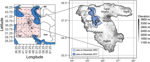
Figure 2. Scatter plot of downscaled versus observed annual precipitation in calibration (1985–2005)

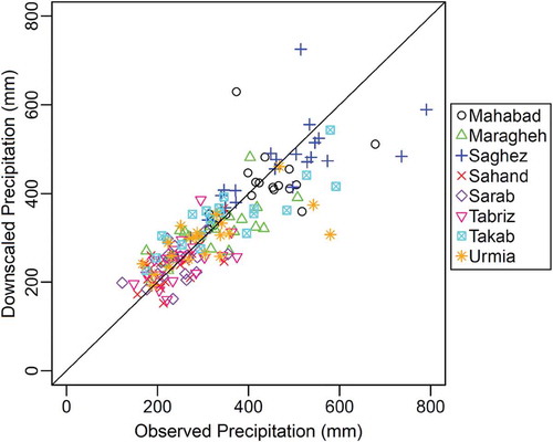
Figure 3. Time series of observed precipitation (triangles) and boxplots of 1000 simulations for downscaled precipitation in calibration (1985–2005) at (a) Mahabad, (b) Maraghe, (c) Saghez, (d) Sahand, (e) Sarab, (f) Tabriz, (g) Takab, and (h) Urmia stations

Figure 4. Scatterplot of downscaled versus observed annual precipitation in leave-one-station-out cross-validation (1985–2005). Vertical lines represent 95% confidence intervals associated with the estimation of the intercept parameter at a new site

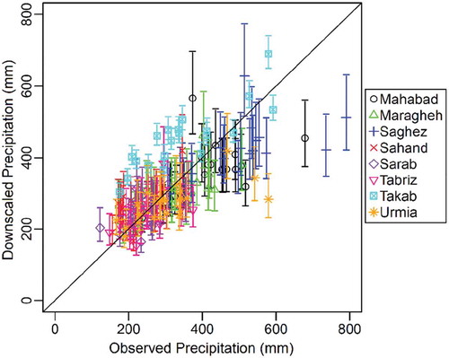
Figure 5. Scatterplots of downscaled versus observed annual precipitation in k-fold cross-validation (1985–1991, 1992–1998, 1999–2005) at Urmia station using (a) MLR and (b) HLM

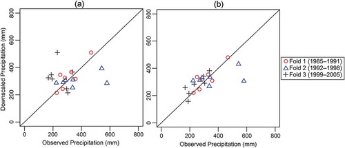
Figure 6. Changes in winter (DJF), spring (DJF), summer (JJA), and autumn (SON) precipitation relative to the historical period based on the multi-model ensemble mean of GCMs under scenarios (a) RCP4.5 2020–2040, (b) RCP4.5 2040–2060, (c) RCP4.5 2060–2080, (d) RCP8.5 2020–2040, (e) RCP8.5 2040–2060, and (f) RCP8.5 2060–2080

Lake Urmia, the terminal lake within the basin, is a hypersaline lake with a surface area of 5 200 km², and a maximum length, width, and depth of 140 km, 55 km, and 16 m, respectively at its original extent. It is the habitat for the Iranian brine shrimp Artemia urmiana which is the primary food source of host water birds. The lake and its islands are protected by the Ramsar Convention on Wetlands of international importance (Fazel et al. 2018). Lake Urmia has faced desiccation since 1995 reaching less than 20% of its original volume by August 2014 (AghaKouchak et al. 2015). Water shortage has resulted in an increase in the salinity from 170 to about 400 g/L (Zarghami and Szidarovszky 2011) while a concentration of 240 g/L or less is suggested to be sustainable for a viable population of Artemia urmiana (Abbaspour and Nazaridoust, 2007). To maintain the lake’s salinity at this sustainable concentration, the water level must be raised by 3 m to the so-called ecological water level, which requires more than 13.2 km³ of water (Sima and Tajrishy 2013). Hamidi-Razi et al. (2018) evaluated several restoration scenarios using a two-dimensional shallow water model. They suggested that the scenarios involving structural practices, such as constructing a dike at the southern part of the lake or transferring water between rivers, would not improve the current condition of the lake. Updating agricultural practices in Lake Urmia basin, however, may lead to partial restoration of the lake. Besides losing Artemia due to increased salinity, salt storms from the lake’s dry bed, land degradation, and biodiversity loss are other environmental consequences of Lake Urmia’s shrinkage that would adversely affect the economy, public health, and agriculture of the surrounding areas (Azarnivand et al. 2015). Some scientists have warned that an outcome similar to that of the Aral Sea is likely for Lake Urmia, but more people would be at risk since the population around Lake Urmia is much larger than around the Aral Sea (AghaKouchak et al. 2015).

3.1 Data

Monthly precipitation data at eight synoptic stations are obtained for the historical period of 1985–2005 from Iran’s Meteorological Organization (www.irimo.ir). The selected sites are quality-controlled stations with the longest record in Lake Urmia basin that contain less than 3% missing data (Table 1). Large-scale climate variables from the National Center for Environmental Prediction/Department of Energy (NCEP/DOE) reanalysis dataset, second version (Kanamitsu et al. 2002) are used for calibrating and validating the downscaling model. This reanalysis product, which is available from 1979 until the present, is treated as an ideal GCM (Cannon and Whitfield 2002).

Table 1. Synoptic stations in Lake Urmia basin

Station name	Latitude (°N)	Longitude (°E)	Elevation (m)	Periods with complete record, 1985–2005
Mahabad	36.75	45.72	1351.8	1985–2005
Maragheh	37.40	46.27	1477.7	1985–2005
Saghez	36.25	46.27	1522.8	1985–2005
Sahand	37.93	46.12	1641.0	1985–1992; 1996–2005
Sarab	37.93	47.53	1682.0	1987–2005
Tabriz	38.08	46.28	1361.0	1985–2005
Takab	36.40	47.10	1817.2	1986–2005
Urmia	37.67	45.05	1328.0	1985–2005

Monthly outputs from eight GCMs participating in the Fifth Phase of the Coupled Model Intercomparison Project (CMIP5) (Table 2) are extracted for the periods of 1985–2005, 2020–2040, 2040–2060, and 2060–2080 (https://esgf-node.llnl.gov). Eight GCMs with varying degrees of bias in simulating precipitation are included such that four GCMs tend to overestimate precipitation over Iran (Access1.0, GISS-E2-H, HadGEM2-CC, and MRI-CGCM3) and four others tend to underestimate it (CanESM2, IPSL-CM5A-MR, MPI-ESM-LR, NorESM1-M) (Abbasian et al. 2018). Also, the selected GCMs are developed by different modelling groups, as climate models from the same groups tend to show similar behaviour (Abbasian et al. 2018). Future scenarios are based on representative concentration pathways RCP4.5 and RCP8.5 emissions scenarios. The former is representative of intermediate scenarios in which the total radiative forcing is stabilized just after 2100, and the latter is a highly energy-intensive scenario resulting from no climate policy, high population growth, and a low rate of technology development leading to increasing greenhouse gas emissions over time. All GCM output variables are re-gridded to the 2.5° by 2.5° grid of the NCEP/DOE reanalysis data using bilinear interpolation.

Table 2. Selected CMIP5 GCMs

Name	Modelling center	Resolution (latitude × longitude)
ACCESS1.0	Commonwealth Scientific and Industrial Research Organization and Bureau of Meteorology, Australia	1.25° × 1.875°
CanESM2	National Centre for Atmospheric Research, Canada	2.7906° × 2.8125°
GISS–E2–H	NASA Goddard Institute for Space Studies, USA	2° × 2.5°
HadGEM2–CC	Met Office Hadley Centre, UK	1.25° × 1.25°
IPSL–CM5A–MR	Institute Pierre-Simon Laplace, France	1.2676° × 2°
MPI–ESM–LR	Max Planck Institute for Meteorology, Germany	1.8653° × 1.875°
MRI–CGCM3	Meteorological Research Institute, Japan	1.12148° × 1.125°
NorESM1–M	Norwegian Climate Centre, Norway	1.8947° × 2.5°

As noted by previous studies, the temporal resolution of the downscaling model is dependent on the purpose of the study. For example, the analysis of extremes would require downscaled products at daily or sub-daily scales (Sachindra and Perera 2016), while monthly or seasonal data is sufficient for water allocation analyses (Sachindra et al. 2014a). As this study aims to project precipitation at a regional scale for long-term planning and management of Lake Urmia basin, the application of the proposed methodology is presented in detail at the annual timescale. The results of the analysis at monthly timescale are outlined in Section 3.8 to briefly investigate the inter-annual changes of precipitation under climate change.

3.2 Specifying atmospheric domain

An atmospheric domain is a region above the study area where large-scale predictors are selected and downscaled to local-scale hydroclimatic variables. The selection of an appropriate size of the domain is important to the downscaling model’s performance. Tripathi et al. (2006), Frost et al. (2011), Sachindra et al. (2013), Mehrotra et al. (2013), and Rashid et al. (2015) chose 6 × 6, 5 × 6, 6 × 7, 3 × 3, and 3 × 4 GCM cells on 2.5° by 2.5° grid systems, respectively. Based on these studies and implementing a trial-and-error procedure, it is concluded that 7 × 7 cells over Lake Urmia basin provide a suitable atmospheric domain. However, considering that the optimal location and dimension of the atmospheric domain can vary from one large-scale predictor to the other (e.g. Wilby et al. 2004, Sachindra et al. 2013), the entire domain is divided into six sub-domains denoted by R0 to R5 in which R0 is the original 7 × 7 area and R5 covers the basin (Fig. 1).

3.3 Selection of optimal predictors

Twenty-one large-scale climate variables are considered as probable predictors (Table 3). All of these predictors are physically connected with local-scale precipitation. Surface precipitation rate, or precipitation flux, defined as the amount of precipitation over the unit area and the unit time, is a predominant predictor in the downscaling process. Some researchers have developed downscaling models with surface precipitation rate being the only predictor. For example, Widmann et al. (2003) and Schmidli et al. (2007) suggested that GCM precipitation outputs are better predictors than GCM atmospheric circulation predictors for downscaling regional precipitation. They claimed that GCM precipitation variables are already physically connected with relevant atmospheric circulation variables; hence, employing GCM precipitation directly as the predictor would be sufficient, and reduces the problems associated with the selection of multiple predictors. However, this idea is subjected to criticism. For example, Jeong et al. (2013) stated that GCM-simulated precipitation tends to show strong systematic biases due to the simplified representation of topography, mesoscale processes, and regional-scale conditions; therefore, it should not be used as the sole downscaling predictor. Notwithstanding, previous studies suggest that surface precipitation can be an effective predictor in statistical downscaling (e.g. Tisseuil et al. 2010, Frost et al. 2011, Jeong et al. 2013, Okkan and Kirdemir 2016, Sachindra and Perera 2016). Precipitation and temperature changes are often related such that higher temperature values are associated with lower precipitation amounts over middle latitudes below 40 °N since higher temperatures favour dry conditions (IPCC 2007). Relative and specific humidity are measures of the atmospheric water vapour content that determines the formation of clouds (Peixoto and Oort 1996). Geopotential heights represent large-scale atmospheric pressure variations. They indicate pressure troughs, regions of relatively low pressure, which are often associated with the formation of clouds and precipitation. Zonal and meridional wind fields determine the movement of precipitation-bearing clouds (Sachindra et al. 2014b).

Table 3. Results of correlation analysis for the set of probable predictors. The atmospheric sub-domain column represents the sub-domain in which each predictor shows the highest correlation with the predictand

Predictor	Abbreviation	Spearman’s correlation	p-value	Atmospheric sub-domain
Air temperature at 500 hPa	air_500hPa	–0.422	0.058	R2
Air temperature at 700 hPa^†	air_700hPa	–0.667	0.001*	R5
Air temperature at 850 hPa	air_850hPa	–0.672	0.001*	R5
Geopotential height at 500 hPa	hgt_500hPa	–0.609	0.004*	R1
Geopotential height at 700 hPa^†	hgt_700hPa	–0.621	0.003*	R1
Geopotential height at 850 hPa	hgt_850hPa	–0.327	0.147	R3
Mean air temperature at 2 m^†	air_2 m	–0.689	0.001*	R3
Mean sea level pressure	mslp	+0.435	0.051	R5
Meridional wind component at 10 m	vwnd_10 m	+0.511	0.019*	R4
Meridional wind component at 500 hPa	vwnd_500hPa	+0.210	0.358	R4
Meridional wind component at 700 hPa	vwnd_700hpa	+0.279	0.219	R4
Meridional wind component at 850 hPa	vwnd_850hPa	+0.584	0.006*	R4
Relative humidity at 500 hPa	rhum_500hPa	+0.597	0.005*	R0
Relative humidity at 700 hPa^†	rhum_700hPa	+0.727	0.000*	R5
Relative humidity at 850 hPa	rhum_850hPa	+0.699	0.000*	R5
Specific humidity at 2 m	shum_2 m	+0.644	0.002*	R5
Surface precipitation rate^†	p-rate	+0.757	0.000*	R5
Zonal wind component at 10 m	uwnd_10 m	–0.297	0.219	R2
Zonal wind component at 500 hPa	uwnd_500hPa	+0.287	0.206	R4
Zonal wind component at 700 hPa^†	uwnd_700hPa	+0.503	0.021*	R4
Zonal wind component at 850 hPa	uwnd_850hPa	+0.501	0.022*	R2

* the sample Spearman’s correlation coefficient is significant at 5% significance level.

^†the predictors pass the partial correlation analysis at the 5% significance level, i.e. the final set of predictors.

Spearman’s correlation coefficient ($\rho$) is used to rank the strength of relationship between each of the 21 predictors and the local January –December total precipitation amounts. For each predictor, the sub-domain that exhibits the highest correlation is identified (Table 3). The optimal sub-domain differs among predictors since some predictors can represent relevant circulation patterns that are not necessarily centred over the study area (Wilby et al. 2004, Sachindra et al. 2014b). For instance, Table 3 shows that annual precipitation has a statistically significant correlation with hgt_700hPa within sub-domain R1, i.e. precipitation amounts can be linked to pressure anomalies at 700 hPa to the north-west of Lake Urmia basin. Predictors which did not pass the two-tailed correlation test at 0.05 significance level were excluded from the analysis. Having screened the predictors using correlation analysis, partial correlation analysis is used to identify and eliminate significant cross-correlations in the set of predictors. Finally, six potential predictors are selected to drive the downscaling model (Table 3).

3.4 Model calibration

Preliminary data analysis using Q-Q plots and Shapiro-Wilk test (Shapiro and Wilk 1965) showed that observed annual precipitation follows normal distribution. In this case, GHLM reduces to HLM, i.e. the link function in Equation (1)(1) $\begin{array}{r}\begin{array}{ccc}& g\left({\mu }_i\right)={\beta }_{j\left[i\right]}^0+{\beta }_{j\left[i\right]}^1{x}_i^1+\cdots +{\beta }_{j\left[i\right]}^k{x}_i^k,& i=1,\cdots ,T,\\ & j=1,\cdots ,S\end{array}\end{array}$(1) is the identity function. Also, the relationship between large-scale predictors and the predictand is examined using scatter plots, which showed a linear relation. In the case of nonlinearity, appropriate predictor transformations should be applied to satisfy the linearity assumption. Large-scale atmospheric potential predictors are standardized prior to downscaling to reduce the bias in the mean and standard deviation of the predictors (Wilby et al. 2004).

Large-scale atmospheric variables are included in the data-level HLM, and latitude, longitude, and elevation, which describe inter-station variability, are considered for the station-level HLM. Consequently, total sample sizes for data and station levels are 162 (8 stations × 21 years) and 8, respectively.

The predictive performance of 10 HLM structures with varying complexities is evaluated using AIC to select the best structure, starting with the simplest model (or the null model M0) (Table 4). The data level of the null model is given by $y_i={\alpha }_{j\left[i\right]}+{ϵ}_i,ϵ{ }_i\sim N\left(0,{\sigma }^2\right),\hspace{0.17em}i=1,\dots ,\hspace{0.17em}162$, with only one parameter (intercept) and no predictors. The parameter variation between stations is characterized in the station level, ${\alpha }_{j\left[i\right]}={\gamma }_0^{\alpha }+{\eta }_j^{\alpha },{\eta }_j^{\alpha }\sim N\left(0,{\tau }^2\right),j=1,\dots ,8,$ with no predictors. Next, the latitudes, longitudes, and elevations of the stations are added to the station-level model M1 as predictors. This results in an increase in AIC indicating that the model is over-parameterized, i.e. some predictors are redundant. Excluding longitude and elevation from the HLM model (i.e. M2) reduces the value of AIC compared to those of M0 and M1 showing that a portion of between-station variability is explained by latitude. This is consistent with previous studies that showed precipitation over Lake Urmia basin would decrease with increasing latitudes and that the effects of longitude and elevation are negligible (Raziei et al. 2008, Fazel et al. 2018). Adding the first and then second predictors with largest correlations with the local precipitation (i.e. surface precipitation rate and relative humidity at 700 hPa) in the data-level HLM (M3 and M4) improves the predictive performance: AIC starts to increase with the addition of other predictors (M5 and M6). In addition, varying-intercept and -slope models (M7–M9) do not improve the overall performance. Consequently, M4 is selected as the optimal HLM structure for downscaling the outputs of GCMs.

Table 4. Different HLM structures and the corresponding AIC values

HLM code	HLM structure	AIC
M0	$\{\begin{array}{lll}{y}_i={\alpha }_{j\left[i\right]}+{ϵ}_i\hfill & {ϵ}_i~N\left(0,{\sigma }^2\right)\hfill & i=1,\dots ,162\hfill \\ {\alpha }_{j\left[i\right]}={\gamma }_0^{\alpha }+{\eta }_j^{\alpha }\hfill & {\eta }_j^{\alpha }~N\left(0,{\tau }^2\right)\hfill & j=1,\dots ,8\hfill \end{array}$	1943
M1	$\{\begin{array}{lll}{y}_i={\alpha }_{j\left[i\right]}+{ϵ}_i\hfill & {ϵ}_i~N\left(0,{\sigma }^2\right)\hfill & i=1,\dots ,162\hfill \\ {\alpha }_{j\left[i\right]}={\gamma }_0^{\alpha }+{\gamma }_1^{\alpha }\left(\text{lat}.\right)+{\gamma }_2^{\alpha }\left(\text{lon}.\right)+{\gamma }_3^{\alpha }\left(\text{eleva}.\right)+{\eta }_j^{\alpha }\hfill & {\eta }_j^{\alpha }~N\left(0,{\tau }^2\right)\hfill & j=1,\dots ,8\hfill \end{array}$	1955
M2	$\{\begin{array}{lll}{y}_i={\alpha }_{j\left[i\right]}+{ϵ}_i\hfill & {ϵ}_i~N\left(0,{\sigma }^2\right)\hfill & i=1,\dots ,162\hfill \\ {\alpha }_{j\left[i\right]}={\gamma }_0^{\alpha }+{\gamma }_1^{\alpha }\left(\text{lat}.\right)+{\eta }_j\hfill & {\eta }_j^{\alpha }~N\left(0,{\tau }^2\right)\hfill & j=1,\dots ,8\hfill \end{array}$	1921
M3	$\{\begin{array}{lll}{y}_i={\alpha }_{j\left[i\right]}+\beta \left(\text{p-rate}\right)+{ϵ}_i\hfill & {ϵ}_i~N\left(0,{\sigma }^2\right)\hfill & i=1,\dots ,162\hfill \\ {\alpha }_{j\left[i\right]}={\gamma }_0^{\alpha }+{\gamma }_1^{\alpha }\left(\text{lat}.\right)+{\eta }_j^{\alpha }\hfill & {\eta }_j^{\alpha }~N\left(0,{\tau }^2\right)\hfill & j=1,\dots ,8\hfill \end{array}$	1851
M4	$\{\begin{array}{lll}{y}_i={\alpha }_{j\left[i\right]}+\beta \left(\text{p-rate}\right)+\zeta \left(\text{rhum}\_\text{700hPa}\right)+{ϵ}_i\hfill & {ϵ}_i~N\left(0,{\sigma }^2\right)\hfill & i=1,\dots ,162\hfill \\ {\alpha }_{j\left[i\right]}={\gamma }_0^{\alpha }+{\gamma }_1^{\alpha }\left(\text{lat}.\right)+{\eta }_j^{\alpha }\hfill & {\eta }_j^{\alpha }~N\left(0,{\tau }^2\right)\hfill & j=1,\dots ,8\hfill \end{array}$	1827
M5	$\{\begin{array}{lll}{y}_i={\alpha }_{j\left[i\right]}+\beta \left(\text{p-rate}\right)+\zeta \left(\text{rhum}\_\text{700hPa}\right)+\xi \left(\text{air}\_\text{2m}\right)+{ϵ}_i\hfill & {ϵ}_i~N\left(0,{\sigma }^2\right)\hfill & i=1,\dots ,162\hfill \\ {\alpha }_{j\left[i\right]}={\gamma }_0^{\alpha }+{\gamma }_1^{\alpha }\left(\text{lat}.\right)+{\eta }_j^{\alpha }\hfill & {\eta }_j^{\alpha }~N\left(0,{\tau }^2\right)\hfill & j=1,\dots ,8\hfill \end{array}$	1839
M6	$\{\begin{array}{lll}{y}_i={\alpha }_{j\left[i\right]}+\beta \left(\text{p-rate}\right)+\zeta \left(\text{rhum}\_\text{700hPa}\right)+\xi \left(\text{air}\_\text{700hPa}\right)+{ϵ}_i\hfill & {ϵ}_i~N\left(0,{\sigma }^2\right)\hfill & i=1,\dots ,162\hfill \\ {\alpha }_{j\left[i\right]}={\gamma }_0^{\alpha }+{\gamma }_1^{\alpha }\left(\text{lat}.\right)+{\eta }_j^{\alpha }\hfill & {\eta }_j^{\alpha }~N\left(0,{\tau }^2\right)\hfill & j=1,\dots ,8\hfill \end{array}$	1841
M7	$\left\{\begin{array}{ccc}{y}_i={\alpha }_{j\left[i\right]}+{\beta }_{j\left[i\right]}\left(\mathrm{p}\text{-}\mathrm{r}\mathrm{a}\mathrm{t}\mathrm{e}\right)+{ϵ}_i& {ϵ}_i\sim N\left(0,{\sigma }^2\right)& i=1,\dots ,162\\ {\alpha }_{j\left[i\right]}={\gamma }_0^{\alpha }+{\gamma }_1^{\alpha }\left(\mathrm{l}\mathrm{a}\mathrm{t}.\right)+{\eta }_j^{\alpha }& {\eta }_j^{\alpha }\sim N\left(0,{\tau }^2\right)& j=1,\dots ,8\\ {\beta }_{j\left[i\right]}={\gamma }_0^{\beta }+{\gamma }_1^{\beta }\left(\mathrm{l}\mathrm{a}\mathrm{t}.\right)+{\eta }_j^{\beta }& {\eta }_j^{\beta }\sim N\left(0,{\upsilon }^2\right)& j=1,\dots ,8\end{array}\right.$	1873
M8	$\left\{\begin{array}{ccc}{y}_i={\alpha }_{j\left[i\right]}+{\beta }_{j\left[i\right]}\left(\mathrm{p}\text{-}\mathrm{r}\mathrm{a}\mathrm{t}\mathrm{e}\right)+\zeta \left(\mathrm{r}\mathrm{h}\mathrm{u}\mathrm{m}\mathrm{\_}700\mathrm{h}\mathrm{P}\mathrm{a}\right)+{ϵ}_i& {ϵ}_i\sim N\left(0,{\sigma }^2\right)& i=1,\dots ,162\\ {\alpha }_{j\left[i\right]}={\gamma }_0^{\alpha }+{\gamma }_1^{\alpha }\left(\mathrm{l}\mathrm{a}\mathrm{t}.\right)+{\eta }_j^{\alpha }& {\eta }_j^{\alpha }\sim N\left(0,{\tau }^2\right)& j=1,\dots ,8\\ {\beta }_{j\left[i\right]}={\gamma }_0^{\beta }+{\gamma }_1^{\beta }\left(\mathrm{l}\mathrm{a}\mathrm{t}.\right)+{\eta }_j^{\beta }& {\eta }_j^{\beta }\sim N\left(0,{\upsilon }^2\right)& j=1,\dots ,8\end{array}\right.$	1842
M9	$\left\{\begin{array}{ccc}{y}_i={\alpha }_{j\left[i\right]}+{\beta }_{j\left[i\right]}\left(\mathrm{p}\text{-}\mathrm{r}\mathrm{a}\mathrm{t}\mathrm{e}\right)+\zeta \left(\mathrm{r}\mathrm{h}\mathrm{u}\mathrm{m}\mathrm{\_}700\mathrm{h}\mathrm{P}\mathrm{a}\right)+{ϵ}_i& {ϵ}_i\sim N\left(0,{\sigma }^2\right)& i=1,\dots ,162\\ {\alpha }_{j\left[i\right]}={\gamma }_0^{\alpha }+{\gamma }_1^{\alpha }\left(\mathrm{l}\mathrm{a}\mathrm{t}.\right)+{\eta }_j^{\alpha }& {\eta }_j^{\alpha }\sim N\left(0,{\tau }^2\right)& j=1,\dots ,8\\ \begin{array}{c}{\beta }_{j\left[i\right]}={\gamma }_0^{\beta }+{\gamma }_1^{\beta }\left(\mathrm{l}\mathrm{a}\mathrm{t}.\right)+{\eta }_j^{\beta }\\ {\zeta }_{j\left[i\right]}={\gamma }_0^{\zeta }+{\gamma }_1^{\zeta }\left(\mathrm{l}\mathrm{a}\mathrm{t}.\right)+{\eta }_j^{\zeta }\end{array}& \begin{array}{c}{\eta }_j^{\beta }\sim N\left(0,{\upsilon }^2\right)\\ {\eta }_j^{\zeta }\sim N\left(0,{\omega }^2\right)\end{array}& \begin{array}{c}j=1,\dots ,8\\ j=1,\dots ,8\end{array}\end{array}\right.$	1886

Note: $y_i$ is the $i$th observed precipitation considering all stations; lat., lon., and eleva.: latitude, longitude and elevation of stations, respectively; ${\alpha }_{j\left[i\right]}$: intercept of the $j$th station which includes the $i$th observation; $\beta$, $\zeta$, and $\xi$: coefficients of p-rate, rhum_700hPa, and air_700hPa respectively, which are constant for all stations; ${\beta }_{j\left[i\right]}$ and ${\zeta }_{j\left[i\right]}$: coefficients of p-rate and rhum_700hPa for the $j$th station which includes the $i$th observed precipitation, respectively; ${\gamma }_0^{\alpha }$, ${\gamma }_0^{\beta }$, and ${\gamma }_0^{\zeta }$: intercept of the station-level regression models for estimating $\alpha$, $\beta$, and $\zeta$, respectively; ${\gamma }_1^{\alpha }$, ${\gamma }_1^{\beta }$, and ${\gamma }_1^{\zeta }$: coefficients of latitude in the station-level regression model for estimating $\alpha$, $\beta$, and $\zeta$, respectively; ${ϵ}_i$: error of the data-level model for the $i$th observed precipitation; ${\eta }_j^{\alpha }$, ${\eta }_j^{\beta }$, and ${\eta }_j^{\zeta }$: error of the station-level models for the $j$th $\alpha$, $\beta$, and $\zeta$, respectively; ${\sigma }^2$, ${\tau }^2$, ${\upsilon }^2$, and ${\omega }^2$: variances of the error terms $ϵ$, ${\eta }^{\alpha }$, ${\eta }^{\beta }$, and ${\eta }^{\zeta }$, respectively.

To further investigate the effectiveness of including surface precipitation rate as a predictor in downscaling precipitation, p-rate is removed from M4 and M5, and these models are re-calibrated with different combinations of the remaining predictors (i.e. rhum_700hPa, air_2m, air_700hPa, hgt_700hPa, uwnd_700hPa). The results show that excluding p-rate can lead to at least 17 units increase in AIC, suggesting that surface precipitation rate is the most influential predictor in the set of large-scale potential predictors. Although the biases in surface precipitation rate are comparatively larger than the biases in some other large-scale variables such as mean air temperature (Abbasian et al. 2018), standardization through subtracting the mean and dividing by the standard deviation prior to downscaling can substantially reduce the biases (Wilby et al. 2004; Sachindra et al. 2013), especially those caused due to overestimation/underestimation and overdispersion/underdispersion.

Examining the standard deviations of the data level (σ) and the station level (τ) can reveal valuable information. Parameter estimation for M4 yields σ = 71.6 mm and τ = 34.7 mm. The estimate of σ shows that within-station variability of precipitation, which cannot be explained by large-scale atmospheric predictors, is 71.6 mm on average. If latitude is removed from the station-level model followed by the re-estimation of parameters, σ does not change since the data-level model’s predictors remain the same. However, τ increases to 88.2 mm indicating that 53.5 mm (60.6%) of between-station variability of precipitation is explained by latitude. The estimate of ${\gamma }_1^{\alpha }$ for M4 suggests that for one degree increase in latitude, annual precipitation decreases by 106.1 mm on average. To illustrate this relationship between latitude and precipitation, the map of the intercepts of the data-level model (α_j) is shown in the Supplementary material (Fig. S1), in which the values of ${\alpha }_j$ are interpolated over the basin from the estimates of ${\alpha }_j,j=1,\cdots ,8$ given by M4. The map shows that the southern regions receive more precipitation on average than the northern parts of the basin. This is because the influence of the Mediterranean air mass, which is the primary source of precipitation over Lake Urmia basin, diminishes over higher latitudes. In this regard, the proposed multi-site downscaling methodology can offer a better understanding of precipitation variability over the study region in the downscaling procedure.

The statistical properties of downscaled annual precipitation using the calibrated HLM based on NCEP/DOE reanalysis dataset and ground-based precipitation data for 1985–2005 are presented in Table 5. The mean bias of the model is –0.9 mm, and it overestimates the minimum by 26.6 mm and underestimates the maximum by 65.5 mm considering all stations together. To illustrate the performance of HLM in calibration, the scatter plot of downscaled precipitation versus the observed annual precipitation is presented in Fig. 2. The Nash-Sutcliffe efficiency coefficient ($C_{\mathrm{N}\mathrm{S}\mathrm{E}}$) and Spearman’s correlation coefficient ($\rho$) values of 0.686 and 0.865 show an overall good model performance (see Supplementary material, Table S1).

Table 5. Statistics of observed annual precipitation (1985–2005), downscaled precipitation using HLM in calibration (1985–2005), downscaled precipitation using HLM in leave-one-station-out cross-validation (1985–2005), and downscaled precipitation using HLM and MLR in k-fold cross-validation (1985–1991, 1992–1998, 1999–2005). SD: standard deviation

Model	Minimum	Mean	Maximum	SD
Observed precipitation	122.5	326.0	790.7	124.2
HLM in calibration	152.1	325.1	725.2	100.9
HLM in leave-one-station-out cross-validation	153.7	323.7	689.4	97.0
HLM in k-fold cross-validation	155.2	323.0	683.3	95.8
MLR in k-fold cross-validation	160.1	322.8	659.6	89.3

The total variance of the predictand is partitioned into the variance explained by the model and the unexplained variance (i.e. model residuals). The stochastic nature of HLM allows for generating an ensemble of downscaled precipitation values based on the unexplained variance to show the uncertainty range of the downscaling process. According to the equation for M4 given in Table 4, the predicted precipitation for the $i$th observation from the $j$th station, $y_i$, follows a normal distribution with mean ${\alpha }_{j\left[i\right]}+\beta \left(\mathrm{p}\text{-}\mathrm{r}\mathrm{a}\mathrm{t}\mathrm{e}\right)+\zeta \left(\mathrm{r}\mathrm{h}\mathrm{u}\mathrm{m}\mathrm{\_}700\mathrm{h}\mathrm{P}\mathrm{a}\right)$ and variance ${\sigma }^2$. Using the distribution of predicted precipitation, 1000 simulations of downscaled precipitation are generated and compared with observations (Fig. 3).

3.5 Model evaluation

As described in Section 2.3, leave-one-station-out cross-validation is used to quantify the predictive performance of the model at new sites (i.e. those not included in calibration). According to M4, the coefficients of p-rate ($\beta$) and rhum_700hPa ($\zeta$) are constant for the entire spatial domain. The intercept, ${\alpha }_{j\left[i\right]}$, which varies between stations, and its associated uncertainties are estimated through the station-level HLM model, ${\alpha }_{j\left[i\right]}={\gamma }_0^{\alpha }+{\gamma }_1^{\alpha }\left(\mathrm{l}\mathrm{a}\mathrm{t}\mathrm{i}\mathrm{t}\mathrm{u}\mathrm{d}\mathrm{e}\right)+{\eta }_j^{\alpha },{\eta }_j^{\alpha }\sim N\left(0,{\tau }^2\right)$. Here, the intercept of the $j$th station follows a normal distribution with mean ${\gamma }_0^{\alpha }+{\gamma }_1^{\alpha }\left(\mathrm{l}\mathrm{a}\mathrm{t}\mathrm{i}\mathrm{t}\mathrm{u}\mathrm{d}\mathrm{e}\right)$ and variance ${\tau }^2$. One thousand simulations are generated from the intercept’s distribution, and precipitation is downscaled based on each generated value to show the confidence intervals associated with estimating the intercept at new sites. Figure 4 presents the scatter plot of downscaled precipitation in the process of leave-one-station-out cross-validation versus the observed annual precipitation. Confidence intervals are not constant among sites since at each step of leave-one-station-out cross-validation different sites participate in calibration leading to different estimates of the variance of the station-level model, ${\tau }^2$. The results show that $C_{\mathrm{N}\mathrm{S}\mathrm{E}}$ and $\rho$ values are 0.512 and 0.761, respectively, for downscaled precipitation at stations not included in calibration (Supplementary material, Table S1), which can indicate the potential capability of HLM as a regional downscaling model. The statistical properties of the downscaled precipitation in leave-one-station-out cross-validation are given in Table 5.

As explained in Section 2.3, k-fold cross-validation is used to assess the out-of-sample predictive performance of the model relative to GLM. Since annual precipitation is normally distributed, GLM reduces to MLR. While HLM can convey information between sites through its station-level model, MLR is not able to establish a link between correlated sites. The historical period (1985–2005) is divided into three sets (1985–1991, 1992–1998, 1999–2005), each of which consists of seven years of data. Since the data-level model of the optimal HLM (M4) contains two predictors (i.e. p-rate and rhum_700hPa), the MLR includes the same two predictors so that the effects of predictor selection on downscaling are eliminated. Focusing on Urmia station as an example, MLR is fitted to data in the first and second sets of Urmia station, and the model is then used to downscale data in the third set of Urmia station. However, HLM is fitted to data in the first and second sets of all stations, and the calibrated HLM is implemented to downscale data in the third set of Urmia station. This process is repeated two other times such that data in the first and second sets of the Urmia station are downscaled as well. The scatter plots of downscaled data using HLM and MLR versus the observed annual precipitation at Urmia station in the historical period are shown in Fig. 5. The plots show that HLM has better performance than MLR as data points obtained from HLM are more tightly scattered around the 1:1 line compared to data points yielded by MLR. The $C_{\mathrm{N}\mathrm{S}\mathrm{E}}$ is 0.438 and –0.249 for HLM and MLR, respectively, supporting the superior performance of HLM. This is due to the fact that MLR uses only 14 data points to estimate the coefficients of predictors and then uses the estimated coefficients to downscale precipitation corresponding to the seven remaining data points. On the other hand, HLM pools data from eight stations for calibration, i.e. HLM involves approximately $14\times 8$ data points to link large-scale predictors with local precipitation, and therefore, can give more reliable estimates of coefficients. The k-fold cross-validation algorithm is applied to all stations, and the statistical properties of downscaled data using HLM and MLR are presented in Table 5. The outputs of MLR exhibit a negative $C_{\mathrm{N}\mathrm{S}\mathrm{E}}$ and almost zero $\rho$ between downscaled and observed annual precipitation, showing poor out-of-sample performance of MLR compared to HLM (Table S1).

3.6 Downscaling precipitation in the historical period from the outputs of GCMs

The outputs of GCMs in 1985–2005 are fed into the calibrated HLM to downscale annual precipitation in the historical period over Lake Urmia basin. The performance of GCMs in reproducing observed annual precipitation is evaluated through scatter plot (see Supplementary material, Fig. S2), $C_{\mathrm{N}\mathrm{S}\mathrm{E}}$, and $\rho$ (Supplementary material, Table S2). The overall $C_{\mathrm{N}\mathrm{S}\mathrm{E}}$ and $\rho$ values, calculated over all data from all stations, are smaller than those obtained from NCEP/DOE reanalysis data. This is because, contrary to GCMs that are not expected to mimic the temporal variations of observed variables at annual or monthly scales, the reanalysis dataset is quality-controlled and corrected based on observations (Christensen et al. 2001). Therefore, the differences between reanalysis dataset and GCMs are attributable to the GCM uncertainties. The maximum $C_{\mathrm{N}\mathrm{S}\mathrm{E}}$ value, associated with GISS-E2-H, is 0.356. The $C_{\mathrm{N}\mathrm{S}\mathrm{E}}$ values for two GCMs, CanESM2 and MRI-CGCM3, are nearly zero (–0.095 and –0.084, respectively).

The predictive mean of the multi-model ensemble is estimated by applying BMA algorithm (Section 2.4) to downscaled precipitation ensembles from the outputs of GCMs. The estimated weights of GCMs in BMA (Table S2) reflect how well GCMs can represent observed annual precipitation relative to each other. GCMs that receive higher BMA weights can represent observations with comparatively more accuracy. For example, GISS-E2–H, with the $C_{\mathrm{N}\mathrm{S}\mathrm{E}}$ value of 0.356 (highest among all) receives the highest weight (0.139), while CanESM2 with the $C_{\mathrm{N}\mathrm{S}\mathrm{E}}$ value of –0.095 takes the second lowest weight (0.115). The multi-model ensemble mean outperforms the individual GCMs with $C_{\mathrm{N}\mathrm{S}\mathrm{E}}$ and $\rho$ values of 0.390 and 0.607, respectively (Supplementary material, Table S2 and Fig. S2).

3.7 Projecting precipitation in the future periods

The outputs of the eight GCMs under RCP4.5 and RCP8.5 climate scenarios in 2020–2040, 2040–2060, and 2060–2080 are used to drive the calibrated HLM to project annual precipitation over Lake Urmia basin. Ensemble members are combined using the BMA algorithm based on parameters estimated for the period 1985–2005, followed by bias correction using the EQM technique (Section 2.5). The underlying assumption of applying BMA weights to ensemble members in the future is that GCMs with a better performance in the historical period can provide more reliable projections of the future. However, modelling climate system involves significant uncertainties, and therefore, putting too much emphasis on single GCMs can lead to misleading conclusions. As a result, none of the GCMs, even those showing relatively poor performance, are excluded from multi-model averaging so that all GCMs contribute to the multi-model ensemble mean to the extent determined by BMA weights. A discussion about the benefits of including both well- and poor-performing models (regarding a historical period) in calculating the multi-model ensemble mean is presented by Weigel et al. (2008). The statistical properties of the bias-corrected multi-model ensemble mean for the future periods and the percentages of change relative to the historical observations are shown in Table 6. For the period 2020–2040, it is projected that annual precipitation amounts will not change under RCP4.5 and will decline by 9.0 mm (2.7%) under RCP8.5. As a result, the next two decades may be viewed as a buffer between the current state and future conditions where precipitation is expected to decrease due to climatic changes. This may give the managers of the basin a reasonable time frame to save the lake before facing the negative impacts of climate change on renewable water resources of Lake Urmia basin. For example, the Urmia Lake Restoration Plan is sticking to a strategy to cut irrigation water use by 40% in the basin. It is a long-term water management plan that is taking the place of a former one that intended to build more reservoirs and develop irrigation. During 2040–2060, it is projected that precipitation will decrease by 19.5 mm (6.0%) and 24.4 mm (7.5%) based on RCP4.5 and RCP8.5, respectively. These amounts of change are not statistically significant according to the two-tailed t-test at the 5% significance level. The largest changes, which are statistically significant, are associated with the period 2060–2080 when projected changes are –36.6 mm (–11.2%) and –50 mm (–15.3%) for RCP4.5 and RCP8.5, respectively. This suggests that Lake Urmia basin may meet water shortage ultimately if effective mitigation plans are not formulated and implemented.

Table 6. Statistics of the bias-corrected multi-model ensemble mean of projected annual precipitation over Lake Urmia basin in the future periods under RCP4.5 and RCP8.5 and the percentage change of the statistics relative to the historical period (in parenthesis)

Scenario	Minimum	Mean	Maximum	SD
RCP4.5 2020–2040	114.4 (–6.6%↓)	325.9 (0.0%)	813.9 (+2.9%↑)	126.0 (+1.4%↑)
RCP4.5 2040–2060	109.7 (–10.5%↓)	306.5 (–6.0%↓)	805.2 (+1.8%↑)	122.3 (–1.5%↓)
RCP4.5 2060–2080	88.6 (–27.7%↓)	289.4* (–11.2%↓)	732.7 (–7.3%↓)	115.4 (–7.1%↓)
RCP8.5 2020–2040	104.0 (–15.1%↓)	317.0 (–2.7%↓)	779.4 (–1.4%↓)	123.0 (–1.0%↓)
RCP8.5 2040–2060	105.6 (–13.8%↓)	301.6 (–7.5%↓)	753.4 (–4.7%↓)	118.5 (–4.6%↓)
RCP8.5 2060–2080	74.5 (–39.2%↓)	276.0* (–15.3%↓)	739.0 (–6.5%↓)	115.0 (–7.4%↓)

* change in mean annual precipitation is significant at the 5% significance level.

3.8 Downscaling precipitation at monthly timescale

The application of the methodology is already described thoroughly at the annual timescale, and the whole process of the proposed multi-site downscaling can be implemented for any desired timescale in accordance with the purpose of a study. However, two important distinctions between annual and sub-annual timescales must be recognized. First, logistic HLM (Section 2.2) may be required to model precipitation occurrence since precipitation may not occur at all time-steps. Second, precipitation amount is a right-skewed variable at sub-annual timescales, and therefore, a GHLM whose predictand is modelled by gamma distribution (Section 2.2) should be used rather than the HLM. The application of the GHLM to downscaling monthly precipitation is described in this section.

October to May are the wet months in that Lake Urmia basin receives precipitation during these months in all years. On the contrary, precipitation may (or may not) occur in June, July, August, and September (dry months). Hence, precipitation occurrence is modelled by logistic HLM, and precipitation amount at wet time steps is predicted through GHLM in June–September. This two-step approach is also very common for downscaling daily precipitation at single sites (Section 1.1.1). In the remaining months, precipitation amount is downscaled at all time steps using GHLM. To model precipitation occurrence, the time series are converted into the binary sequence of 0s and 1s, where 0 and 1 represent dry and wet time-steps, respectively.

The correlation analysis followed by partial correlation analysis in all months reveals that surface precipitation rate, relative humidity, and air temperature are the most influential large-scale predictors for both occurrence and amount models. Repeating predictor selection on a seasonal basis: winter (DJF), spring (MAM), summer (JJA), and autumn (SON), which is suggested by some authors (e.g. Fealy and Sweeney 2007, Mehrotra and Sharma 2010, Jeong et al. 2013), does not significantly affect the final set of potential predictors. Prior to model calibration, predictors are normalized, and the validity of linear relationship between predictors and local monthly precipitation is verified. Several logistic HLMs and GHLMs with different degrees of complexity are fitted to the data, and the optimal models are identified based on AIC for each month. This process is fully described in Section 3.4.

The final result of downscaling monthly precipitation from the reanalysis dataset is illustrated in Fig. S3 in the Supplementary material. The $C_{\mathrm{N}\mathrm{S}\mathrm{E}}$ and $\rho$ values between the downscaled and observed data are 0.672 and 0.866, respectively. The calibrated models are driven by the outputs of GCMs in the historical period, and the weights of GCMs to calculate the multi-model ensemble mean are obtained by BMA algorithm. The RCP experiments of the GCMs are then employed to downscale monthly precipitation over future periods. The ensemble members from GCMs are combined and bias-corrected using BMA and EQM, respectively. Examining future projection of precipitation by the multi-model ensemble mean shows that the dry months of the year (June–September) will not shift in the future.

The changes in winter, spring, summer, and autumn precipitation in the future periods under RCP4.5 and RCP8.5 relative to the historical period projected by the multi-model ensemble mean of GCMs are presented in Fig. 6. About 45% of average annual precipitation (326 mm) is observed in spring in which agricultural production is highly reliant on precipitation conditions (Nassiri et al. 2006, Nouri et al. 2017). Against this background, the most dramatic changes in the future are expected to occur in spring (up to –12 mm in 2060–2080). This can intensify water withdrawal and diversion upstream of Lake Urmia to meet crop demand in spring, and therefore, further complicate revitalizing the lake.

4 Summary and concluding remarks

The main objective of this paper is to propose the Generalized Hierarchical Linear Model (GHLM) to downscale precipitation at multiple sites. GHLM is structured into at least two levels: the data level explains within-group variability of the predictand (precipitation variability at stations), and the group level describes between-group variability (precipitation variability between sites). The predictand of GHLM can follow the exponential family of distributions such as gamma and normal distributions for continuous variables and Bernoulli distribution for discrete variables. This allows for modelling precipitation occurrence and precipitation amount at sub-annual timescales in which precipitation may not occur at all time steps, and precipitation amount is not normally distributed. For the case of normally distributed predictand such as annual precipitation in this study, GHLM reduces to hierarchical linear model (HLM). The methodology is demonstrated by downscaling annual and monthly precipitation over Lake Urmia basin in the northwest of Iran. Lake Urmia is already undergoing  severe desiccation partly due to unfavourable climate conditions during the past decades, and any decline in precipitation under climate change can decrease runoff ending up in the lake, and therefore, hinder the restoration of the lake.

Leave-one-station-out cross-validation shows that the methodology has good performance in regionalization, i.e. it can downscale precipitation at locations not included in model calibration. This stems from the fact that GHLM can explain a portion of the spatial variability of precipitation field through its group-level model. k-fold cross-validation reveals that the out-of-sample predictive performance of the proposed model is superior to multiple linear regression, which cannot transfer information between sites. Taking between-station correlations into account, GHLM can pool data from neighbouring sites to build a more reliable link between large-scale climate variables and local precipitation.

The bias-corrected multi-model ensemble mean projects a slight reduction in precipitation in the near future (2020–2040). However, a declining trend will lead to 11.2% and 15.3% decline in annual precipitation over 2060–2080 based on RCP4.5 and RC8.5 climate scenarios, respectively. The results show that the largest decline in precipitation will occur in spring when agriculture is highly dependent on precipitation.

Disclosure statement

No potential conflict of interest was reported by the authors.

Supplementary material

Supplemental data for this article can be accessed here.

References

- Abbasian, M., Moghim, S., and Abrishamchi, A., 2018. Performance of the general circulation models in simulating temperature and precipitation over Iran. Theoretical and Applied Climatology, 135 (3–4), 1465–1483. doi:10.1007/s00704-018-2456-y.
- Abbaspour, M. and Nazaridoust, A., 2007. Determination of environmental water requirements of Lake Urmia, Iran: an ecological approach. International Journal of Environmental, 64 (2), 161–169. doi:10.1080/00207230701238416.
- AghaKouchak, A., et al., 2015. Aral Sea syndrome desiccates Lake Urmia: call for action. Journal of Great Lakes Research, 41 (1), 307–311. doi:10.1016/j.jglr.2014.12.007.
- Akaike, H., 1974. A new look at the statistical model identification. IEEE Transactions on Automatic Control, 19 (6), 716–723. doi:10.1109/tac.1974.1100705.
- Alizadeh-Choobari, O., et al., 2016. Climate change and anthropogenic impacts on the rapid shrinkage of Lake Urmia. International Journal of Climatology, 36 (13), 4276–4286. doi:10.1002/joc.4630.
- Azarnivand, A., Hashemi-Madani, F., and Banihabib, M., 2015. Extended fuzzy analytic hierarchy process approach in water and environmental management (case study: lake Urmia Basin, Iran). Environmental Earth Sciences, 73 (1), 13–26. doi:10.1007/s12665-014-3391-6.
- Baigorria, G.A. and Jones, J.W., 2010. GiST: A stochastic model for generating spatially and temporally correlated daily rainfall data. Journal of Climate, 23 (22), 5990–6008. doi:10.1175/2010jcli3537.1.
- Bardossy, A. and Plate, E.J., 1992. Space–time models for daily rainfall using atmospheric circulation patterns. Water Resources Research, 28 (5), 1247–1259. doi:10.1029/91wr02589.
- Bates, D., et al., 2015. Fitting Linear Mixed-Effects Models Using lme4. Journal of Statistical Software, 67 (1), 1. doi:10.18637/jss.v067.i01.
- Beecham, S., Rashid, M., and Chowdhury, R.K., 2014. Statistical downscaling of multi-site daily rainfall in a South Australian catchment using a Generalized Linear Model. International Journal of Climatology, 34 (14), 3654–3670. doi:10.1002/joc.3933.
- Booker, D. and Dunbar, M., 2008. Predicting river width, depth and velocity at ungauged sites in England and Wales using multilevel models. Hydrological Processes, 22 (20), 4049–4057. doi:10.1002/hyp.7007.
- Cannon, A. and Whitfield, P., 2002. Downscaling recent streamflow conditions in British Columbia, Canada using ensemble neural network models. Journal of Hydrology, 259 (1–4), 136–151. doi:10.1016/s0022-1694(01)00581-9.
- Chandler, R.E., 2002. Generalized linear modelling for daily climate time series (software and user guide). London, England: Department of Statistical Science, University College London.
- Chaudhari, S., et al., 2018. Climate and anthropogenic contributions to the desiccation of the second largest saline lake in the twentieth century. Journal of Hydrology, 560, 342–353. doi:10.1016/j.jhydrol.2018.03.034
- Christensen, O.B., et al., 2001. Internal variability of regional climate models. Climate Dynamics, 17 (11), 875–887. doi:10.1007/s003820100154.
- Clarke, R., 2001. Separation of year and site effects by generalized linear models in regionalization of annual floods. Water Resources Research, 37 (4), 979–986. doi:10.1029/2000wr900370.
- Das, J. and Umamahesh, N.V., 2016. Downscaling monsoon rainfall over river godavari basin under different climate-change scenarios. Water Resources Management, 30 (15), 5575–5587. doi:10.1007/s11269-016-1549-6.
- Dempster, A.P., Laird, N.M., and Rubin, D.B., 1977. Maximum likelihood from incomplete data via the EM algorithm. Journal of the Royal Statistical Society, 39B, 1–39.
- Duan, Q., et al., 2007. Multi-model ensemble hydrologic prediction using Bayesian model averaging. Advances in Water Resources, 30 (5), 1371–1386. doi:10.1016/j.advwatres.2006.11.014.
- Fazel, N., et al., 2018. Regionalization of precipitation characteristics in Iran’s Lake Urmia basin. Theoretical and Applied Climatology, 132 (1–2), 363–373. doi:10.1007/s00704-017-2090-0.
- Fealy, R. and Sweeney, J., 2007. Statistical downscaling of precipitation for a selection of sites in Ireland employing a generalised linear modelling approach. International Journal of Climatology, 27 (15), 2083–2094. doi:10.1002/joc.1506.
- Frost, A., et al., 2011. A comparison of multi-site daily rainfall downscaling techniques under Australian conditions. Journal of Hydrology, 408 (1–2), 1–18. doi:10.1016/j.jhydrol.2011.06.021.
- Fu, G., Chiew, F.H.S., and Shi, X., 2018. Generation of multi-site stochastic daily rainfall with four weather generators: a case study of Gloucester catchment in Australia. Theoretical and Applied Climatology, 134 (3–4), 1027–1046. doi:10.1007/s00704-017-2306-3.
- Furrer, E. and Katz, R., 2007. Generalized linear modelling approach to stochastic weather generators. Climate Research, 34, 129–144. doi:10.3354/cr034129
- Gelman, A. and Hill, J., 2007. Data analysis using regression and multilevel/hierarchical models. Cambridge: University Press. doi:10.1017/cbo9780511790942
- Goly, A., Teegavarapu, R.S.V., and Mondal, A., 2014. Development and evaluation of statistical downscaling models for monthly precipitation. Earth Interactions, 18 (18), 1–28. doi:10.1175/ei-d-14-0024.1.
- Hamidi-Razi, H., et al., 2018. Investigating the restoration of Lake Urmia using a numerical modelling approach. Journal of Great Lakes Research. doi:10.1016/j.jglr.2018.10.002
- Hanel, M. and Buishand, T., 2015. Assessment of the sources of variation in changes of precipitation characteristics over the rhine basin using a linear mixed-effects model. Journal of Climate, 28 (17), 6903–6919. doi:10.1175/jcli-d-14-00775.1.
- Harpham, C. and Wilby, R.L., 2005. Multi-site downscaling of heavy daily precipitation occurrence and amounts. Journal of Hydrology, 312 (1–4), 235–255. doi:10.1016/j.jhydrol.2005.02.020.
- Harrold, T.I., Sharma, A., and Sheather, S.J., 2003. A non-parametric model for stochastic generation of daily rainfall occurrence. Water Resources Research, 39 (10), 1300. doi:10.1029/2003wr002182.
- Hayhoe, H., 2000. Improvements of stochastic weather data generators for diverse climates. Climate Research, 14, 75–87. doi:10.3354/cr014075
- Hoeting, J.A., et al., 1999. Bayesian model averaging: a tutorial. Statistical Science, 14 (4), 382–417.
- IPCC. 2007. Climate change 2007: the physical science basis. contribution of working group i to the fourth assessment report of the intergovernmental panel on climate change [Solomon, S., D. Qin, M. Manning, Z. Chen, M. Marquis, K.B. Averyt, M. Tignor and H.L. Miller (eds.)]. Cambridge, United Kingdom and New York, NY, USA: Cambridge University Press, 996.
- Jeong, D., et al., 2013. A multi-site statistical downscaling model for daily precipitation using global scale GCM precipitation outputs. International Journal of Climatology, 33 (10), 2431–2447. doi:10.1002/joc.3598.
- Jones, R.G., et al., 2004. Generating high resolution climate change scenarios using PRECIS. Exeter: Met Office Hadley Centre.
- Kamruzzaman, M., Beecham, S., and Metcalfe, A., 2016. Estimation of trends in rainfall extremes with mixed effects models. Atmospheric Research, 168, 24–32. doi:10.1016/j.atmosres.2015.08.018
- Kanamitsu, M., et al., 2002. NCEP–DOE AMIP-II Reanalysis (R-2). B. AmBulletin of the American Meteorological Society, 83 (11), 1631–1643. doi:<1631:nar>10.1175/BAMS-83-11-1631.
- Kannan, S. and Ghosh, S., 2013. A nonparametric kernel regression model for downscaling multisite daily precipitation in the Mahanadi basin. Water Resources Research, 49 (3), 1360–1385. doi:10.1002/wrcr.20118.
- Khazaei, B., et al., 2019. Climatic or regionally induced by humans? Tracing hydro-climatic and land-use changes to better understand the Lake Urmia tragedy. Journal of Hydrology, 569, 203–217. doi:10.1016/j.jhydrol.2018.12.004
- Kim, Y., et al., 2012. Reducing overdispersion in stochastic weather generators using a generalized linear modelling approach. Climate Research, 53 (1), 13–24. doi:10.3354/cr01071.
- Kleiber, W., Katz, R.W., and Rajagopalan, B., 2012. Daily spatiotemporal precipitation simulation using latent and transformed Gaussian processes. Water Resources Research, 48 (1), 1. doi:10.1029/2011wr011105.
- Kleiber, W., Katz, R.W., and Rajagopalan, B., 2013. Daily minimum and maximum temperature simulation over complex terrain. The Annals of Applied Statistics, 7 (1), 588–612. doi:10.1214/12-aoas602.
- Lee, T., Ouarda, T.B.M.J., and Jeong, C., 2012. Nonparametric multivariate weather generator and an extreme value theory for bandwidth selection. Journal of Hydrology, 452-453, 161–171. doi:10.1016/j.jhydrol.2012.05.047
- Lessels, J.S. and Bishop, T.F.A., 2013. Estimating water quality using linear mixed models with stream discharge and turbidity. Journal of Hydrology, 498, 13–22. doi:10.1016/j.jhydrol.2013.06.006
- Li, H., Sheffield, J., and Wood, E., 2010. Bias correction of monthly precipitation and temperature fields from Intergovernmental panel on climate change AR4 models using equidistant quantile matching. Journal of Geophysical Research, 115, D10. doi:10.1029/2009jd012882
- Liang, Z., et al., 2013. Application of bayesian model averaging approach to multimodel ensemble hydrologic forecasting. Journal of Hydrologic Engineering, 18 (11), 1426–1436. doi:10.1061/(asce)he.1943-5584.0000493.
- Lin, G.-F., Chang, M.-J., and Wu, J.-T., 2016. A hybrid statistical downscaling method based on the classification of rainfall patterns. Water Resources Management, 31 (1), 377–401. doi:10.1007/s11269-016-1532-2.
- Liu, W., et al., 2012. A comparison of three multi-site statistical downscaling models for daily rainfall in the North China Plain. Theoretical and Applied Climatology, 111 (3–4), 585–600. doi:10.1007/s00704-012-0692-0.
- Loukas, A., Vasiliades, L., and Tzabiras, J., 2008. Climate change effects on drought severity. Advances in Geosciences, 17, 23–29. doi:10.5194/adgeo-17-23-2008
- Mandal, S., Srivastav, R.K., and Simonovic, S.P., 2016. Use of beta regression for statistical downscaling of precipitation in the Campbell River basin, British Columbia, Canada. Journal of Hydrology, 538, 49–62. doi:10.1016/j.jhydrol.2016.04.009
- Maurer, E. and Pierce, D., 2014. Bias correction can modify climate model simulated precipitation changes without adverse effect on the ensemble mean. Hydrology and Earth System Sciences, 18 (3), 915–925. doi:10.5194/hess-18-915-2014.
- Mehrotra, R. and Sharma, A., 2006. Conditional resampling of hydrologic time series using multiple predictor variables: A K-nearest neighbour approach. Advances in Water Resources, 29 (7), 987–999. doi:10.1016/j.advwatres.2005.08.007.
- Mehrotra, R. and Sharma, A., 2010. Development and application of a multisite rainfall stochastic downscaling framework for climate change impact assessment. Water Resources Research, 46 (7), W07526. doi:10.1029/2009wr008423.
- Mehrotra, R. and Sharma, A., 2016. A multivariate quantile-matching bias correction approach with auto- and cross-dependence across multiple time scales: implications for downscaling. Journal of Climate, 29 (10), 3519–3539. doi:10.1175/jcli-d-15-0356.1.
- Mehrotra, R., et al., 2013. Assessing future rainfall projections using multiple GCMs and a multi-site stochastic downscaling model. Journal of Hydrology, 488, 84–100. doi:10.1016/j.jhydrol.2013.02.046
- Mehrotra, R., Srikanthan, R., and Sharma, A., 2006. A comparison of three stochastic multi-site precipitation occurrence generators. Journal of Hydrology, 331 (1–2), 280–292. doi:10.1016/j.jhydrol.2006.05.016.
- Nahar, J., Johnson, F., and Sharma, A., 2017. Assessing the extent of non-stationary biases in GCMs. Journal of Hydrology, 549, 148–162. doi:10.1016/j.jhydrol.2017.03.045
- Najafi, M.R. and Moradkhani, H., 2016. Ensemble Combination of Seasonal Streamflow Forecasts. Journal of Hydrologic Engineering, 21 (1), 04015043. doi:10.1061/(asce)he.1943-5584.0001250.
- Nash, J. and Sutcliffe, J., 1970. River flow forecasting through conceptual models part I — A discussion of principles. Journal of Hydrology, 10 (3), 282–290. doi:10.1016/0022-1694(70)90255-6.
- Nasseri, M., Tavakol-Davani, H., and Zahraie, B., 2013. Performance assessment of different data mining methods in statistical downscaling of daily precipitation. Journal of Hydrology, 492, 1–14. doi:10.1016/j.jhydrol.2013.04.017
- Nassiri, M., et al., 2006. Potential impact of climate change on rainfed wheat production in Iran. Archives of Agronomy and Soil Science, 52 (1), 113–124. doi:10.1080/03650340600560053.
- Nouri, M., Homaee, M., and Bannayan, M., 2017. Climate variability impacts on rainfed cereal yields in west and northwest Iran. International Journal of Biometeorology, 61 (9), 1571–1583. doi:10.1007/s00484-017-1336-y.
- Okkan, U. and Kirdemir, U., 2016. Downscaling of monthly precipitation using CMIP5 climate models operated under RCPs. Meteorological Applications, 23 (3), 514–528. doi:10.1002/met.1575.
- Pang, B., et al., 2017. Statistical downscaling of temperature with the random forest model. Advances in Meteorology, 2017, 1–11. doi:10.1155/2017/7265178
- Peel, M.C., Finlayson, B.L., and McMahon, T.A., 2007. Updated world map of the Köppen-Geiger climate classification. Hydrology and Earth System Sciences, 11 (5), 1633–1644. doi:10.5194/hess-11-1633-2007.
- Peixoto, J. and Oort, A., 1996. The climatology of relative humidity in the atmosphere. Journal of Climate, 9 (12), 3443–3463. doi:10.1175/1520-0442(1996)009<3443:tcorhi>2.0.co;2.
- Qian, B., Corte-Real, J., and Xu, H., 2002. Multisite stochastic weather models for impact studies. International Journal of Climatology, 22 (11), 1377–1397. doi:10.1002/joc.808.
- Raftery, A., et al., 2005. Using Bayesian Model Averaging to Calibrate Forecast Ensembles. Monthly Weather Review, 133 (5), 1155–1174. doi:10.1175/mwr2906.1.
- Rajagopalan, B. and Lall, U., 1999. A K-nearest neighbour simulator for daily precipitation and other weather variables. Water Resources Research, 35 (10), 3089–3101. doi:10.1029/1999wr900028.
- Rashid, M., Beecham, S., and Chowdhury, R., 2015. Statistical downscaling of CMIP5 outputs for projecting future changes in rainfall in the Onkaparinga catchment. Science of the Total, Environment 530-531, 171–182. doi:10.1016/j.scitotenv.2015.05.024
- Raudenbush, S.W. and Bryk, A.S., 2002. Hierarchical linear models applications and data analysis methods. 2nd. Thousand Oaks: Sage.
- Raziei, T., Bordi, I., and Pereira, L., 2008. A precipitation-based regionalization for Western Iran and regional drought variability. Hydrology and Earth System Sciences, 12 (6), 1309–1321. doi:10.5194/hess-12-1309-2008.
- Sachindra, D., et al., 2013. Least square support vector and multi-linear regression for statistically downscaling general circulation model outputs to catchment streamflows. International Journal of Climatology, 33 (5), 1087–1106. doi:10.1002/joc.3493.
- Sachindra, D., et al., 2014a. Statistical downscaling of general circulation model outputs to precipitation-part 2: bias-correction and future projections. International Journal of Climatology, 34 (11), 3282–3303. doi:10.1002/joc.3915.
- Sachindra, D., et al., 2014b. Statistical downscaling of general circulation model outputs to precipitation-part 1: calibration and validation. International Journal of Climatology, 34 (11), 3264–3281. doi:10.1002/joc.3914.
- Sachindra, D. and Perera, B., 2016. Annual statistical downscaling of precipitation and evaporation and monthly disaggregation. Theoretical and Applied Climatology, 131 (1–2), 181–200. doi:10.1007/s00704-016-1968-6.
- Samadi, S., et al., 2012. Statistical downscaling of river runoff in a semi arid catchment. Water resource management, 27 (1), 117–136. doi:10.1007/s11269-012-0170-6.
- Schmidli, J., et al., 2007. Statistical and dynamical downscaling of precipitation: an evaluation and comparison of scenarios for the European Alps. Journal of Geophysical Research, 112 (D4), D4. doi:10.1029/2005jd007026.
- Semenov, M.A. and Barrow, E.M., 1997. Use of a stochastic weather generator in the development of climate change scenarios. Climatic Change, 35 (4), 397–414. doi:10.1023/A:1005342632279.
- Shadkam, S., et al., 2016. Impacts of climate change and water resources development on the declining inflow into Iran’s Urmia Lake. Journal of Great Lakes Research, 42 (5), 942–952. doi:10.1016/j.jglr.2016.07.033.
- Shapiro, S.S. and Wilk, M.B., 1965. An analysis of variance test for normality (complete samples). Biometrika, 52 (3–4), 591–611. doi:10.1093/biomet/52.3-4.591.
- Sharif, M. and Burn, D.H., 2007. Improved K-nearest neighbor weather generating model. Journal of Hydrologic Engineering, 12 (1), 42–51. doi:10.1061/(asce)1084-0699(2007)12:1(42).
- Sima, S. and Tajrishy, M., 2013. Using satellite data to extract volume–area–elevation relationships for Urmia Lake, Iran. Journal of Great Lakes Research, 39 (1), 90–99. doi:10.1016/j.jglr.2012.12.013.
- Slaets, J., et al., 2014. A turbidity-based method to continuously monitor sediment, carbon and nitrogen flows in mountainous watersheds. Journal of Hydrology, 513, 45–57. doi:10.1016/j.jhydrol.2014.03.034
- Srivastav, R.K., Schardong, A., and Simonovic, S.P., 2014. Equidistance quantile matching method for updating IDFCurves under climate change. Water Resource Management, 28 (9), 2539–2562. doi:10.1007/s11269-014-0626-y.
- Stern, R.D. and Coe, R., 1984. A model fitting analysis of daily rainfall data. Journal of the Royal Statistical Society. Series A (General), 147 (1), 1–34. doi:10.2307/2981736.
- Tisseuil, C., et al., 2010. Statistical downscaling of river flows. Journal of Hydrology, 385 (1–4), 279–291. doi:10.1016/j.jhydrol.2010.02.030.
- Tripathi, S., Srinivas, V., and Nanjundiah, R., 2006. Downscaling of precipitation for climate change scenarios: A support vector machine approach. Journal of Hydrology, 330 (3–4), 621–640. doi:10.1016/j.jhydrol.2006.04.030.
- Verdin, A., et al., 2015. Coupled stochastic weather generation using spatial and generalized linear models. Stochastic Environmental Research and Risk Assessment, 29 (2), 347–356. doi:10.1007/s00477-014-0911-6.
- Verdin, A., et al., 2018. A conditional stochastic weather generator for seasonal to multi-decadal simulations. Journal of Hydrology, 556, 835–846. doi:10.1016/j.jhydrol.2015.12.036
- Verdin, A., et al., 2019. BayGEN: A Bayesian space‐time stochastic weather generator. Water Resources Research, 55 (4), 2900–2915. doi:10.1029/2017wr022473.
- Weigel, A.P., Liniger, M.A., and Appenzeller, C., 2008. Can multi-model combination really enhance the prediction skill of probabilistic ensemble forecasts?. Quarterly Journal of the Royal Meteorological Society, 134 (630), 241–260. doi:10.1002/qj.210.
- Widmann, M., Bretherton, C., and Salathé, E., 2003. Statistical precipitation downscaling over the northwestern united states using numerically simulated precipitation as a predictor. Journal of Climate, 16 (5), 799–816. doi:10.1175/1520-0442(2003)016<0799:spdotn>2.0.co;2.
- Wilby, R., Dawson, C., and Barrow, E., 2002. sdsm — a decision support tool for the assessment of regional climate change impacts. Environmental Modelling & Software, 17 (2), 145–157. doi:10.1016/s1364-8152(01)00060-3.
- Wilby, R. and Harris, I., 2006. A framework for assessing uncertainties in climate change impacts: low-flow scenarios for the River Thames, UK. Water Resources Research, 42 (2), 2. doi:10.1029/2005wr004065.
- Wilby, R.L., et al., 2004. Guidelines for use of climate scenarios developed from statistical downscaling methods. IPCC Task Group on Data and Scenario Support for Impact and Climate Analysis (TGICA). https://www.ipcc-data.org/guidelines/dgm_no2_v1_09_2004.pdf
- Wilks, D., 2011. Statistical Methods in the Atmospheric Sciences. Elsevier Academic Press, Amsterdam. doi:10.1016/c2010-0-65519-2
- Wilks, D.S., 1998. Multisite generalization of a daily stochastic precipitation generation model. Journal of Hydrology, 210 (1–4), 178–191. doi:10.1016/s0022-1694(98)00186-3.
- Woolhiser, D.A., 1992. Modeling daily precipitation – progress and problems. In: A.T. Walden and P. Guttorp, eds. Statistics in the Environmental and Earth Sciences. New York: Wiley, 71–89.
- Zarghami, M. and Szidarovszky, F., 2011. Multicriteria analysis: applications to water and environment management. Berlin: Springer. doi:10.1007/978-3-642-17937-2