Assessing the origin and processes controlling groundwater salinization in coastal aquifers through integrated hydrochemical, isotopic and hydrogeochemical modelling techniques

ABSTRACT

The origin of groundwater and the processes controlling its chemical composition in complex coastal aquifers are of interest, as about 44% of the world’s population lives in coastal areas. Groundwater over-exploitation in the highly urbanized coastal regions has exerted pressure on these aquifers, leading to seawater intrusion. This study aimed to identify (1) the complex relationship between natural and anthropogenic factors, and (2) the hydrogeochemical processes controlling the groundwater chemistry in an over-stressed coastal aquifer of southern India. The results indicate an increase in the extent of seawater intrusion from 4 km in 1969 to 17 km in 2014. Major hydrogeochemical processes controlling the aquifers are evaporation, ion exchange and dissolution of aluminosilicates, gypsum, halites and calcites. The integrated use of field investigation with hydrochemical, isotopic and hydrogeochemical modelling techniques allowed a conceptual model of the groundwater salinization process over 46 years to be developed as a basis for designing sustainable management measures.

KEYWORDS:

• Cl/Br ratio
• stable isotopes
• hydrogeochemical model
• PHREEQC
• seawater intrusion
• Chennai
• India

Editor S. Archfield Associate editor M. Hutchins

1 Introduction

Seawater intrusion (SWI) in coastal regions is a global phenomenon. With about 44% of the world’s population living within 150 km of the coast (Reed 2010), groundwater abstraction is high in the coastal aquifers as it is the main reliable source of freshwater in these areas. The problem is more pronounced in tropical regions with monsoonal rains where the availability of surface water resources is limited. Due to the low topography, coastal aquifers are highly sensitive to fluctuations in groundwater pumping and recharge. Hence, over-exploitation of groundwater is the major contributor to aquifer salinization in the coastal areas (Kim et al. 2003, Askri et al. 2016, Alfarrah et al. 2017). The seawater–freshwater dynamics is also influenced by natural processes including coastal evolution, long-term historical sea-level changes, tsunami, flooding and climate change.

Several methods are available to explore the dynamics and position of the seawater–freshwater interface. Numerical modelling and geophysical investigations are increasingly adopted to identify the extent of SWI (Hwang et al. 2004, Kazakis et al. 2016, Rajaveni et al. 2016a, 2016b). But when seawater mixes with freshwater, the interaction causes changes in the chemical composition of fresh groundwater. Understanding the hydrogeochemical processes is essential to assess the origin and evolution of salinity along the flowpath, which are generally not considered during numerical modelling. Determination of the electrical conductivity (EC), major ions (especially sodium and chloride), minor ions (especially bromide) and isotopes in groundwater are the important indicators in understanding SWI processes. These parameters are widely assessed and the SWI is deciphered by using graphical approaches. Various ionic ratios are also used as SWI indicators (Alcalá and Custodio 2008, Lee et al. 2008, Nair et al. 2016). Kazakis et al. (2016) used geophysical data in areas where hydrochemical data could not be collected to delineate SWI. Bouzourra et al. (2015) used hydrochemical data in conjunction with historical information and adopted multivariate statistical methods to identify SWI processes. A multi-isotope approach was adopted by Cary et al. (2015) to evaluate groundwater salinization in coastal aquifers.

In most SWI studies, hydrochemical data collected during a short term is used (Gemitzi et al. 2014, Alfarrah et al. 2017, Bagheri et al. 2017, Maurya et al. 2019). To understand the complex processes and mechanisms that control SWI in an area, however, long-term assessment of the hydrochemical characteristics is required. Especially in coastal areas with tropical climate which mainly depend on monsoons for groundwater recharge, water levels fluctuate widely. Further, in these areas groundwater is over-exploited and SWI is highly dynamic in nature. In such a scenario, it is vital to use an integrated approach to understanding SWI by including the long-term variation in hydrochemistry. The mixing processes in coastal aquifers and the vulnerability of the aquifer to SWI can be better determined only through long-term monitoring and analysis of hydrochemical data (Kazakis et al. 2016). Additionally, hydrogeochemical modelling should be used to identify the processes that are likely to take place during SWI. The advantage of hydrochemical models is that historical data can be used along with recently collected data to identify the long-term processes along the groundwater flow direction leading to salinization of the aquifer.

This study was carried out to determine the complex relationship between natural and anthropogenic factors and to identify the processes controlling the groundwater chemistry in a highly stressed and environmentally sensitive coastal aquifer, in order to properly manage the available fresh groundwater resources. The site chosen for this study, located north of Chennai, southern India, is perhaps the world’s most affected region due to SWI. The novelty of this study is the application of an interdisciplinary approach through field investigation, hydrochemical analysis, isotopic analysis and hydrogeochemical modelling by long-term monitoring and assessment of SWI in a coastal aquifer with tropical monsoon climate. It enables us to demarcate the interaction between seawater and freshwater and to understand the processes of seawater–freshwater mixing. Though the novel approach is explained with a case study, the method and the interpretations from this study can be adapted globally to any coastal region. This study is of great environmental significance, as it can be used as a detailed baseline to frame strategies to improve groundwater quality with time.

2 Study area

The study area forms a part of the Arani and Koratalaiyar (A-K) river basin, southern India (578 km²) (Fig. 1). The A-K rivers are non-perennial and flow only for a few days during the northeast monsoon. The Bay of Bengal lies on the eastern side. The Buckingham canal, used in the past for navigation purposes, is located almost parallel to the Bay of Bengal at about 3 km from the coast, and it carries ingress saline water. Characterized by a tropical wet and dry climate, summer (April to June) temperatures range from 38°C to 45°C and winter (November to January) temperatures range from 18°C to 29°C. The mean annual rainfall is 1200 mm. About 60% of this is from the northeast monsoon (October to December), and 35% is from the southwest monsoon (June to September). The maximum elevation is about 10 m a.m.s.l. in the west and at sea level in the eastern boundary. The drainage pattern is dendritic to sub-dendritic (Supplementary material Fig. S1(a)).

Geologically, this area comprises rocks from Archaean to Quaternary age (Fig. 1). Crystalline rocks of Archaean age comprising gneiss, granite and charnockite form the basement (Rao et al. 2004). The Satyavedu Formation, containing shale and clay deposits of the Upper Gondwana, overlies the basement. A massive pile of lacustrine and fluvial deposits overlies the Upper Gondwana formation with an unconformity. This is overlaid by shale, clay, sandstone and marine sediments of the Tertiary Period. The Quaternary strata, which are the youngest of the series, comprise laterite and alluvium deposits. A small patch of laterite is present on the northwestern part of the study area.

Figure 1. Location of the study area indicating sampling points

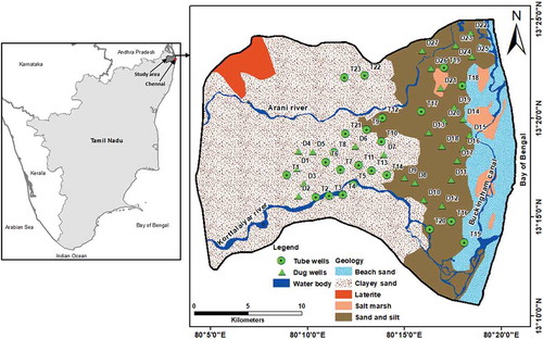
Alluvial deposits consist of fine to coarse sand, gravel with pebbles, clayey sand, sandy clay, and clay, which occur mostly along the two river courses due to the migration of rivers. These deposits form a complex irregular conglomeration with a clay layer, which are mainly deposited in the fluvial and marine environments. The thickness of the alluvium is around 60 m and it increases towards the east. This formation has a clay layer of about 3 to 5 m in thickness, which functions as an aquitard allowing some vertical transfer of water. Hence, the aquifer is multi-layered with an unconfined upper aquifer (UA) and a semi-confined lower aquifer (LA). The thin layer of clay extends up to about 30 km inland from the coast. There are eight different land uses in the study area: agriculture, aquaculture, built-up area, forest, water bodies, saltpans, wasteland and wetland (see Supplementary material, Fig. S1(b)). The region is predominantly used for agricultural purposes, and the water demand is mostly met by groundwater.

3 Methodology

3.1 Groundwater sampling and analysis

Groundwater samples were collected once every 2 months from 50 monitoring locations (28 open wells from the UA and 22 tube wells from the LA) from June 2011 to December 2014. Groundwater level (m) was measured using a water level indicator (Solinist 101). EC and pH were measured in the field using a multi-parameter portable instrument (YSI 556 MPS) calibrated with appropriate standards. Groundwater samples were collected after pumping the well until the measured EC was reasonably stable. Carbonate and bicarbonate concentrations were measured immediately after sample collection by titration using the alkalinity test kit (Merck 1.11109.0001). Samples were collected by filtering through a 0.2-mm filter paper into 1-L polyethylene (HDPE) bottles (pre-washed with dilute hydrochloric acid). Bottles were rinsed three times with the water sample before filling the bottle with the sample and were labeled. Filtered samples were analysed for calcium, magnesium, sodium, potassium, chloride, sulphate and bromide using an ion chromatograph (Metrohm 861). Adequate care was taken to ensure that the analytical procedures, precision, quality assurance and quality control were adopted. The ion balance error was calculated to check the accuracy of the analysis and was found to be within ±5%. During pre-monsoon in 2018, the EC was measured in these wells to compare the extent of salinization.

Initially, 22 samples were collected in March and May 2012 for isotope analysis (Nair et al. 2015). However, this study did not consider seasonal fluctuations as the samples were collected only during the summer (pre-monsoon). From the preliminary results of Nair et al. (2015), nine locations were chosen for further isotope analysis in June and December 2013. Additionally, one sample was collected from the Buckingham Canal and the mouth of Arani River. Stable isotopes (δD, δ¹⁸O) were analysed using a PICARRO L1102-i isotope analyser. The International Atomic Energy Agency (IAEA) standards were used for calibration.

3.2 Hydrogeochemical modelling

Hydrogeochemical models are based on equilibrium concepts and are used to predict the spatial and temporal variation in chemical reactions that occur along the groundwater flowpath (Bethke 1996). The hydrogeochemical modelling code PHREEQC (Parkhurst and Appelo 1999) was used to understand the interaction of groundwater with the aquifer material. PHREEQC was initially used to identify the hydrogeochemical processes occurring in the study area by inverse modelling. Subsequently, forward modelling was used to predict the temporal variation in the concentration of ions in groundwater due to mixing of seawater, taking into consideration the hydrogeochemical processes identified from inverse modelling. Saturation indices (SI) for different minerals were also calculated using PHREEQC.

3.2.1 Inverse modelling

The purpose of inverse modelling is to identify the processes that have resulted in the present groundwater quality. By assuming two solutions (groundwater samples) as the initial and final composition along a flowpath or from different times, inverse modelling can be used to identify the chemical processes that occur as groundwater evolves along the flowpath (Parkhurst and Appelo 1999). In this study, first the different groundwater types were identified. Groundwater samples from July 2014 were plotted on a Piper diagram. This time was chosen as it was the most recent representation of groundwater quality in the study area. The Piper plot indicated three major water types. Out of these three types of water, two samples from each type were chosen such that they lie along the groundwater flowpath, and inverse modelling was performed.

3.2.2 Forward modelling

Forward modelling predicts the water composition and mass transfer based on hypothesized geochemical reactions (Plummer 1992). The one-dimensional geochemical solute transport model was set up for 25 km inland from the coast. The model was developed based on the following hydrogeological characteristics of the LA: hydraulic gradient = 0.005, hydraulic conductivity = 150 m/d (UNDP 1987), porosity = 20%. With a time step of 1 month, the length of each cell was calculated as 112.5 m. Boundary conditions were assumed to be flux boundaries. The diffusion coefficient was considered to be 1 × 10⁻⁹ m²/s based on the surface and subsurface lithology (UNDP 1987), and the dispersivity was considered to be 60 m (Charalambous and Garratt 2009).

In the eastern part, it is assumed that the first 3 km is filled with seawater. The chemical characteristics of seawater were arrived at based on the analysis of seawater collected from four locations. The average concentration of these samples was used as the chemistry of seawater. The concentration of ions in groundwater in the western part of the study area is based on the secondary data collected from the United Nations Development Programme in 1969. Validation of the model was carried out for the following time periods based on data availability: 1975 (from the Chennai Metro Water Supply and Sewerage Board), from 1987 to 2007 (from the Public Works Department) and from 2011 to 2014 (present study). The geochemical processes identified by inverse modelling were also accounted during forward modelling.

4 Results and discussion

4.1 Groundwater variation

Rainfall contributes to the majority of groundwater recharge. Irrigation return flow and seepage from rivers and water storage bodies such as ponds and reservoirs also contribute a minor portion of the recharge (Rajaveni et al. 2016a, 2016b). Rainfall recharge in the alluvial formations of this area varies from 15 to 27%. Spatial variation of groundwater head in the UA varies from –2 to 10 m a.m.s.l. during pre-monsoon, and it varies from –1.09 to 14 m a.m.s.l. during post-monsoon. Spatial variation in groundwater head of the LA varies from –32.4 to 0.5 m a.m.s.l. during pre-monsoon, and from –27.9 to 0.6 m a.m.s.l. during post-monsoon. Overall, the maximum water level is observed after the wet season in December and January, and a rapid decline in water levels is observed during the dry season from April to June. In dry years with low rainfall, the abstraction rate exceeds the recharge and the difference is met by groundwater storage depletion (UNDP 1987). Fluctuation in groundwater head is greater in the LA than the UA due to heavy pumping.

4.2 Hydrochemistry

The pH varies from 7.5 to 8.9, indicating that the groundwater is mostly alkaline. The relative distribution of cations and anions in groundwater was in the following order: sodium > calcium > magnesium > potassium and chloride > sulphate > bicarbonate > carbonate. Na-Cl was the major groundwater type. It was predominant in the pre-monsoon, and a few samples had mixed Ca-Mg-Cl groundwater type. During the post-monsoon, Ca-Mg-Cl, Ca-HCO₃ and Na-HCO₃ types were also noticed. Neither the UA nor the LA showed significant variation in the major groundwater type.

In general, calcium and magnesium in groundwater are mainly due to the dissolution of aquifer material. A high concentration of sodium is a common phenomenon in coastal regions, and the concentration increases when proximity to the sea increases. The concentration of potassium was the lowest among the major cations studied (Supplementary material, Table S1). The amount of carbonate was negligible. Thus, it is mainly bicarbonate that contributes to the alkaline nature of the water. Bicarbonate content was abundant in the recharge areas (freshwater) and decreased towards the discharge areas (coastal groundwater). Chloride, like sodium, occurs frequently in seawater-intruded areas. Similar behaviour of sodium and chloride ions indicates a common source (Alcalá and Custodio 2008, Lee et al. 2008, Nair et al. 2013). Sulphate is mainly contributed by aquifer-water interaction and leachate from sewage. Sulphate reduction is commonly reported due to low rainfall in this area (Sathish 2013). Spatially, all ions measured in groundwater were found in high concentrations in the eastern part (i.e. towards the coast), and the concentrations decreased towards the west.

4.3 Electrical conductivity

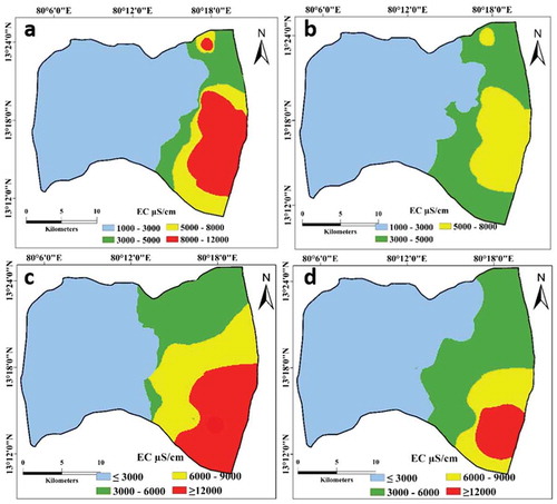
The range of EC in groundwater was 425–24 512 µS/cm (Table S1). Generally, EC > 3000 µS/cm encountered in the coastal areas is considered a contribution from SWI. Significant spatial and temporal variation in the EC of the UA and the LA was observed (Fig. 2). Temporally, EC is influenced by the rainfall pattern. High rainfall leads to a low concentration of EC in both the UA and the LA. The extent of SWI was traced through the interpretation of spatial variation in EC. The northern part of the study area had EC ranging between 1250 and 6000 µS/cm. Also, the effect of SWI is not significant in the post-monsoon period in the north, where EC is generally < 3000 µS/cm (Fig. 2(b) and (d)). But coastal areas in the south of the study area had EC values consistently above 3000 µS/cm, i.e. ranging from 8000 to 15, 000 µS/cm (Fig. 2(a–d)). Such high EC values compared to the other parts is not only contributed by lateral SWI, but also due to saltwater recharge from saltpans located in the southern part and the saline backwaters. Over the study period, EC in the UA was > 3000 µS/cm up to 15 km from the coast, and in the LA it extended up to 17 km inland from the coast (Table 1).

Figure 2. Spatial variation in electrical conductivity (EC) in the upper aquifer in (a) July 2014 and (b) December 2014, and in the lower aquifer in (c) July 2014 and (d) December 2014

4.4 Historical chloride and sodium concentration

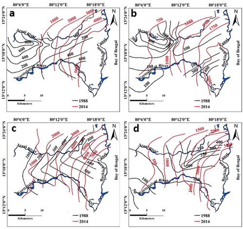
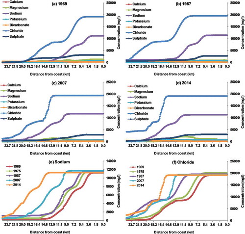
The sodium and chloride concentrations measured in groundwater during this study were compared with a previous study conducted in 1988 (Elango 1992) to understand the changes in the hydrochemical status over the past three decades. Though the sampling wells in the two studies are not the same, the comparison indicated an increase by about 10-fold in the concentrations of chloride and sodium. The spatial variation in the measured chloride and sodium in groundwater during 1988 and 2014 is shown in Fig. 3. Since the river flows for only 0–30 d/year, groundwater major ion concentrations were indicated as contours even across the rivers (Fig. 3). The impact of SWI caused by increased pumping of groundwater for the needs of the growing population is obvious. In 1988, the groundwater of the UA had high concentrations of chloride (Fig. 3(a)) and sodium in the southern part (Fig. 3(b)). The LA in 1988 possessed comparatively elevated contents of these ions in the north (Fig. 3(c and d)). The minor difference in the spatial variation of sodium and chloride in groundwater between 1988 and 2014 is due to some changes in sampling locations.

Figure 3. Temporal variation in the concentration of ions in the upper aquifer: (a) chloride and (b) sodium; and in the lower aquifer: (c) chloride and (d) sodium

4.5 Hydrochemical evolution

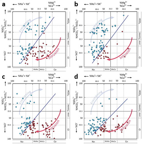
A plot of EC versus chloride was used to derive information on SWI graphically. Figure 4 shows most samples as fresh, whereas some of them are mixed with and influenced by intruding seawater. Seasonal fluctuation is also observed, as the percentage of mixing of seawater varies due to monsoonal effects (Fig. 4(a and b)). A Hydrochemical Facies Evolution diagram (HFE-D) (Gimenez-Forcada and Roman 2015) was used to understand the influence of SWI on the groundwater (Fig. 5). Samples falling in the lower left column (i.e. towards 100% sodium and chloride) indicate the influence of seawater (Fig. 5). Recharge of freshwater in the western part of the area and its lateral entry into the LA leads to freshening of groundwater in the LA (Fig. 5(c and d)). A higher salinization process in the UA and the LA during pre-monsoon is established, in concurrence with the other indicators. This is indicated by a shifting of points from the intruded zone to the freshening zone. Similar effects also occur in the UA, indicating the effect of rainfall recharge.

Figure 4. Plot of electrical conductivity vs. chloride showing normal groundwater conditions, saltwater intrusion and mixing for (a) July (pre-monsoon) and (b) December (post-monsoon)

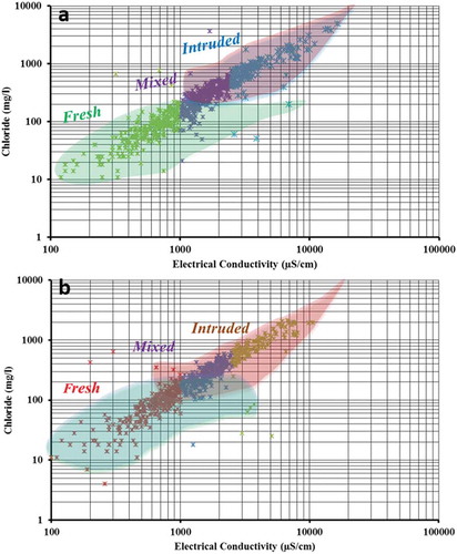
Figure 5. Hydrochemical facies evolution showing aquifer freshening and salinization in the upper aquifer in (a) July 2014 and (b) December 2014, and in the lower aquifer in (c) July 2014 and (d) December 2014

4.6 Seawater intrusion indicators

4.6.1 Na/Cl ratio

The Na/Cl ratio is used to differentiate between SWI and other sources of saltwater. Na/Cl molar ratio < 0.86 (Mæller 1990) indicates SWI (marked as intruded areas in Fig. S2) and > 1 typically characterizes anthropogenic sources like domestic wastewater (Jones et al. 1999). Sodium replaces calcium in the aquifer matrix through reverse ion exchange in advance of the SWI. This reduces the sodium concentration from groundwater, and the Na/Cl ratio drops (Appelo and Postma 2005). Thus, low Na/Cl ratios combined with other geochemical parameters serve as an early indicator to predict the onset of saltwater intrusion. The extent of SWI in the UA ranged up to 15 km during the pre-monsoon and up to 10 km during the post-monsoon (Fig. S2(a–h)). In the LA, the extent of the ingress of seawater ranged up to 17 km during the pre-monsoon and up to 16 km during the post-monsoon (Table 1; Fig. S2(i–p)). Usually, in the pre-monsoon period, the LA is affected by SWI along the entire coast (northern and southern parts). However, after the monsoons, the northern part of the study area is less affected than the southern region. Unlike the LA, the UA is characterized by a high Na/Cl ratio only in the southern region (Fig. S2). The high electropositive nature of sodium in the seawater mixing front means it is readily depleted by taking part in the reverse ion exchange process. Thus, apart from dilution, the reverse ion exchange process also plays a major role in determining the Na/Cl ratio in the post-monsoon period.

Table 1. Extent of seawater intrusion indicated by various indices in different time periods

		Extent of seawater intrusion (km)
		Upper aquifer				Lower aquifer
Indicator	Months	2011	2012	2013	2014	2011	2012	2013	2014	Remarks
EC	July	14.5	15.0	14.0	12.0	15.5	17.0	16.2	16.8	EC > 3000 µS/cm (Kim et al. 2003)
	Dec	10.9	11.0	10	10.5	13.5	14.2	14.7	13.5
Na/Cl	July	15.0	14.0	14.0	13.8	16.6	17.0	16.9	16.8	Na/Cl = 0.86 is seawater, Na/Cl between 0.86 and 1 is mixed water, Na/Cl < 1 is freshwater (Vengosh and Pankratov 1998)
	Dec	9.0	9.5	10.1	10.3	15.9	13.6	14.1	14.1
Cl/Br	July	13.3	14.5	13.4	13.8	16.0	17. 5	16.4	16.8	Cl/Br = 297 is seawater, Cl/Br > 297 is hypersaline water (Davis et al. 1998)
	Dec	10.3	11.9	11.3	11.5	13.9	14.7	13.2	13.7
BEX	July	12.7	13.3	12.2	12.9	14.7	16.3	15.2	15.9	BEX < 0 is seawater (Stuyfzand 2008)
	Dec	10.8	12.0	11.1	11.4	12.4	12.5	12.7	13.1

BEX: base exchange index; EC: electrical conductivity.

4.6.2 Cl/Br ratio

The Cl/Br ratio in seawater around the world is relatively constant (Cl/Br = 292) (Hem 1992). Minor variations in this ratio for seawater (290 ± 4) due to local effects have been reported (Krauskopf 1979, Davis et al. 1998, Panno et al. 2006, Alcalá and Custodio 2008). The Cl/Br ratio of groundwater in the study area varies from 100 to 800. Areas with Cl/Br >300, indicating SWI, are considered as intruded areas (Fig. S3.) Values above the seawater Cl/Br ratio are observed in wells located closer to the sea, and the ratio decreases towards the west. These high values indicate recharge of evaporated seawater from the salt pans and backwaters in the rivers and the canal. The highest Cl/Br ratio, of 800, was observed in the LA (July 2011) at about 7 km from the coast. Groundwater quality was comparatively better in the northern part than the south. The maximum extent of SWI in the UA was up to 14.5 km from the coast in the pre-monsoon, whereas the highest during the post-monsoon was about 12 km (Table 1). The LA was more affected by SWI than the UA, with the maximum SWI extending up to 17.5 km during the pre-monsoon and up to 15 km during the post-monsoon (Table 1).

4.6.3 Base exchange indices

The relationship of sodium, potassium and magnesium to chloride can be used to identify the salinization process and freshening of groundwater using the base exchange indices (BEX) (Versluys 1916, 1931, Schoeller 1934, 1956). The exchange reaction assumes that intruding seawater displaces freshwater, or vice versa, and during this process sodium (during salinization) or calcium (during freshening) is adsorbed. This reaction is given as follows (Stuyfzand 2008):

(1) $2\mathrm{N}{\mathrm{a}}^{+}+\mathrm{C}\mathrm{a}-\mathrm{E}\mathrm{X}\mathrm{C}\mathrm{H}\stackrel{\leftharpoonup }{\rightharpoondown }\mathrm{N}{\mathrm{a}}^{2+}+2\mathrm{N}\mathrm{a}-\mathrm{E}\mathrm{X}\mathrm{C}\mathrm{H}$(1)

where EXCH is the base exchanger (eg. clay, peat), and the left and right arrows indicate salinization (SWI) and freshening (freshwater intrusion), respectively.

For aquifer systems without dolomite, such as in this study area, the BEX index (meq/L) is used (Stuyfzand 1986):

(2) $\mathrm{B}\mathrm{E}\mathrm{X}=\mathrm{N}\mathrm{a}+\mathrm{K}+\mathrm{M}\mathrm{g}-1.0716\mathrm{C}\mathrm{l}$(2)

A salinization trend (BEX < 0) is detected in the southern part due to SWI from extensive groundwater pumping. BEX increases towards the west (BEX > 0) in both the UA (Fig. S4(a and b)) and the LA (Fig. S4(c and d)) indicating the freshening of groundwater. The extent of SWI identified through BEX is given in Table 1.

4.7 Stable isotopes

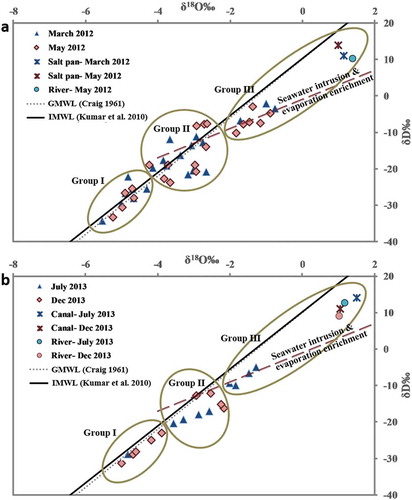
During 2012, the δ¹⁸O value of the groundwater samples ranged from –5.5‰ to –0.8‰, and the δD ranged from –34.2‰ to –2.1‰ (Nair et al. 2015, Nair 2016). In 2013, the δ¹⁸O value ranged from –5.0‰ to –1.3‰ and the δD ranged from –31.3‰ to –5.1‰. To characterize isotopic samples, the global meteoric water line (GMWL) – a regression line (δD = 8.0 × δ¹⁸O + 10) suggested by IAEA protocol – is usually used (Craig 1961). However, the current study uses the Indian meteoric water line (IMWL), a regression line suggested by Kumar et al. (2010) (δD = 7.82 × δ¹⁸O + 10.22) based on the precipitation samples taken from major locations in southern India. The evaporation enrichment line is calculated with δD = 4.9 × δ¹⁸O – 1.

The samples were characterized into three groups (Fig. 6). In Group I, the samples fall on the IMWL towards the depleted region. They are isotopically lighter and are considered to be recharge water derived from rainfall. Group II samples are intermediate between recharge water and isotopically enriched waters. This is the mixed zone, with a mixture of rainfall-derived groundwater and seawater (Nair et al. 2015, Nair 2016). Groundwater samples in Group III plot between IMWL and the evaporation line. They are located close to the sea and are enriched with heavy isotopes. The samples falling below and on the evaporation line follow a linear trend showing mixing with a similar source enriched with heavy isotopes. Such samples enriched due to SWI and recharge of the evaporated enriched water normally move towards the positive side (upward direction). Surface-water samples from the Arani river, Buckingham Canal and salt pans are enriched and cluster under Group III.

Temporal variation in the isotopic signatures of the samples collected in 2012 (both in the pre-monsoon) show the migration of few samples from Group II to Group III (Fig. 6(a)). This enrichment is related to low recharge, saline ingress from the sea and a high evaporation rate experienced during the peak summer month (May) (Nair et al. 2015, Nair 2016). All samples in 2013 fall below the IMWL (Fig. 6(b)) and pre- and post-monsoon samples exhibit a similar trend. Samples from December 2013 were more depleted than in July 2013 due to the monsoon effect. With no samples falling exactly on the IMWL, it is evident that evaporation and mixing with seawater/groundwater enriched in heavy isotopes are major processes controlling the groundwater composition.

Figure 6. Temporal variation in stable isotopes for (a) March and May 2012 and (b) July and December 2013, indicating the three groups of groundwater evolution: Group I – groundwater recharged by rainfall; Group II – mixed zone, i.e. mixture of rainfall derived from groundwater and seawater; and Group III – groundwater enriched due to seawater intrusion and evaporation. Canal: the Buckingham Canal; River: mouth of Arani River; GMWL: global meteoric water line; and IMWL: Indian meteoric water line

4.8 Hydrogeochemical processes and geochemical modelling

The physical process of SWI is accompanied by various hydrogeochemical processes in the coastal aquifers. Before inverse modelling, it is necessary to know the hydrogeochemical processes occurring in this area. These were identified by the direct analysis of the chemical composition of groundwater samples using bivariate plots. Inference from this analysis was used as an input in the inverse model.

Evaporation increases the concentration of all mineral species in water and the salinity of the soil zone. A plot of calcium versus bicarbonate (Fig. S5(a)) in groundwater was compared with the groundwater evaporation line of lowest ionic concentration. Most of the samples plot along this line, indicating the dominance of evaporation. The recharging rainwater and irrigation return-flow are subjected to evaporation, which increases the concentration before it reaches the water table. Further, there are several large-diameter open wells in the region from which evaporation can take place. The evaporation-enriched groundwater from the UA moves to the LA due to the increase in groundwater pumping from the LA over the years.

Sodium and chloride are the dominant ions in seawater, but fresh groundwater in the coastal aquifers is often dominated by calcium and bicarbonate ions resulting from the dissolution of calcite (Appelo and Postma 2005). Sodium is taken up by the exchanger, whereas calcium is released into water (a process indicated as salinization in Equation (1))(1) $2\mathrm{N}{\mathrm{a}}^{+}+\mathrm{C}\mathrm{a}-\mathrm{E}\mathrm{X}\mathrm{C}\mathrm{H}\stackrel{\leftharpoonup }{\rightharpoondown }\mathrm{N}{\mathrm{a}}^{2+}+2\mathrm{N}\mathrm{a}-\mathrm{E}\mathrm{X}\mathrm{C}\mathrm{H}$(1) . If the flux of fresh groundwater is prominent during the monsoon, a reverse cation exchange reaction takes place (a process indicated as freshening in Equation 1(1) $2\mathrm{N}{\mathrm{a}}^{+}+\mathrm{C}\mathrm{a}-\mathrm{E}\mathrm{X}\mathrm{C}\mathrm{H}\stackrel{\leftharpoonup }{\rightharpoondown }\mathrm{N}{\mathrm{a}}^{2+}+2\mathrm{N}\mathrm{a}-\mathrm{E}\mathrm{X}\mathrm{C}\mathrm{H}$(1) ), resulting in the enrichment of sodium relative to chloride (Appelo and Postma 2005).

During SWI, due to its conservative nature, chloride usually remains without change. But, in comparison with chloride, sodium begins to decrease. This is shown in the plot of chloride versus sodium in groundwater samples in different time periods, along with the seawater–freshwater mixing line (Figure S5 b – f). Most of the groundwater samples fall above or on the hypothetical seawater–freshwater mixing line, indicating an obvious increase in the sodium concentration with respect to chloride. Also, as the sampling year increases, more samples plot below the seawater–freshwater mixing line, indicating depletion of sodium and SWI. This is more pronounced in 2007 and 2014 (Fig. S5(e and f)).

The SI was calculated for various minerals from the 1980s to 2014. The SI of gypsum ranged from –2 to 0.5 with an average of 0.2 (Fig. S6), the SI of calcite ranged from –1 to 0.7 and the SI of dolomite ranged from –1 to 0.75. Minerals like gypsum, dolomite and calcite showed a cyclic variation of precipitation and dissolution processes, whereas halite has always been under-saturated since 1980.

4.8.1 Inverse model

As the SWI is more pronounced in the LA and as this aquifer is extensively pumped, hydrogeochemical modelling was carried out for the LA. A Piper plot (Fig. S7) of groundwater samples collected during July 2014 indicated three major water types. Two samples from each water type lying along the groundwater flowpath were chosen. They are divided into three zones: Zone 1, samples of Ca-HCO₃ type in the west (inland T1 and T2); Zone 2, samples of CaNaHCO₃ type in the northeastern coastal part (T22, T23); and Zone 3, samples of Na-Cl water type in the southeast (T15, T16) of the study area (see Fig. 1 for the location of the samples; the groundwater type is given in Fig. S7). These three pairs of solutions were considered the initial and final solutions for the inverse modelling, i.e. samples from the west (Zone 1) are considered the initial solution, which undergoes certain hydrogeochemical processes to evolve to the groundwater composition of Zone 2 or Zone 3 along the flow direction. The aquifer consists of clayey sand, sandy clay, gravel, sand and clay. Hence, the presence of aluminosilicates was considered. Halite and gypsum were also noticed in some locations of the study area and were included in the model. During inverse modelling, the water was assumed to react with aluminosilicates, calcite, dolomite, gypsum and halite, in addition to the processes such as ion exchange identified through the bivariate plots. The mineral phases and the total dissolved solids (TDS) of groundwater in the three zones are given in Table 2.

4.8.2 Forward modelling and simulation

The concentrations of the ions used for forward modelling are given in Table 3. The simulated concentrations of the major ions in groundwater through forward modelling are given in Fig. 7(a–f). Predicted sodium and chloride ions obtained along the flow direction in 1969 indicate SWI up to 3.9 km from the coast (Fig. 7(a)). The trend was similar in 1975 with an increase in SWI up to 5.5 km (Fig. 7(e and f)). The extent of SWI was about 6 km in 1987 (Fig. 7(b)), which was on par with the 7 km SWI reported earlier (UNDP 1987). SWI was noted at 11 km in 2007 (Fig. 7(c)). The overall trend of major ions in groundwater in 2014 is similar to that during the other time periods (Fig. 7(d)). The extent of SWI (spatial) and the temporal variation in sodium and chloride concentration shows high salinity in groundwater during the year 2014, which is in line with the results from the other methods adopted.

Table 2. Mineral phases and total dissolved solids (TDS) in the groundwater of the three zones. Zone 1: western part; Zone 2: northeast; Zone 3: southeast

Minerals/TDS	Zone 1	Zone 2	Zone 3
Albite	0.26	23.56	16.12
Calcite	2.59	-	-
CaX2	–5.07	–3.00	–2.15
CO2g	2.63	11.23	5.59
Gypsum	-	5.48	2.64
Halite	3.43	92.36	35.23
Illite	–0.09	–11.37	–6.93
Quartz	–0.24	–31.93	–23.57
NaX	8.14	-	-
KX	-	6.01	4.30
TDS measured (mg/L)	1300	3554	10 452
TDS computed (mg/L)	1360	3741	10 610

Table 3. Physical and chemical characteristics of seawater and groundwater used in forward modelling. Chemical composition in mg/L

		Groundwater composition in the western part
Parameter	Seawater (eastern part)	1969	1975	1987	2007	2014
pH	8.5	7.2	7	7.4	7	7
pe	8	4	4	4	4	4
Density (kg/m^3)	1.025	1	1	1	1	1
Calcium	400	60	58	79	65	129
Magnesium	1200	12	42.5	60	97.5	70
Sodium	11 200	50.2	135	186	221	414
Potassium	720	4.7	12.6	18.5	11.2	9.8
Bicarbonate	183	355	500	510	289	348
Chloride	19 990	170.9	270	298	265	268
Sulphate	3767	39.9	89	101	56	55.6

Figure 7. Simulated spatial variation in the concentration of major ions for (a) December 1969, (b) December 1987, (c) December 2007 and (d) December 2014. Simulated spatial variation in the concentration of (e) sodium and (f) chloride during different periods

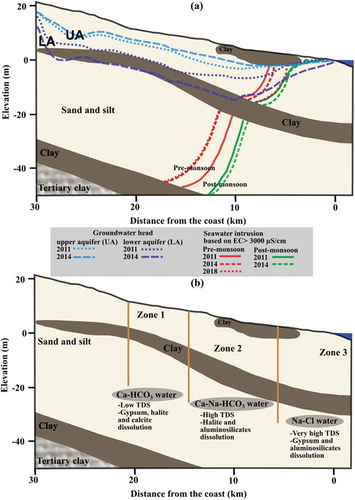
The extent of SWI identified from isotope composition, chemical contents of ions, SWI indices, processes identified through inverse modelling and direct analysis of the hydrochemical data are summarized into a conceptual hydrogeological model for this area (Fig. 8(a and b)). Zone 1 indicates the exchange reactions between NaX and CAX₂, dissolution of evaporites (gypsum and halite) and dissolution of calcite resulting in the exchange of major cations. The TDS of groundwater was also comparatively low (Table 2). In Zone 2, hydrolysis of aluminosilicates (albite, illite) from the silty clay layer is one of the major processes that increases the TDS and controls the chemistry of groundwater. Dissolution of halite is the additional process resulting in the salinization of groundwater in Zone 2. This leads to the sharp increase in chloride, sulphate and bicarbonate contents. Similar to Zone 2, aluminosilicate hydrolysis and gypsum dissolution were the dominant processes that contributed to the groundwater salinity in Zone 3. In addition to these geochemical processes, the mixing of seawater has resulted in a significant increase in TDS, from 1300 to 10 452 mg/L (Table 2). In general, dissolution of evaporites and cation exchange reactions govern the hydrochemistry in the west (Zone 1), whereas aluminosilicate hydrolysis and evaporite dissolution were the dominant hydrogeochemical processes contributing to groundwater salinization in the northeast (Zone 2) and the southeast (Zone 3) (Table 2; Fig. 8(b)).

Figure 8. (a) Conceptual diagram of the seawater–freshwater interface showing the extent of seawater intrusion at different times. (b) Conceptual west-to-east cross section showing the identified geochemical processes

5 Conclusion

Overexploitation of groundwater and subsequent salinization of the groundwater due to SWI is often reported in coastal aquifers. The vulnerability of the highly stressed coastal aquifers to contamination and the demarcation of areas affected by SWI are normally carried out using short-term data collected once or twice during a year. However, the complex geochemical processes controlling the origin of salinization can be assessed only through long-term monitoring of hydrochemical data. Each method of SWI identification depends on certain principles and thus the inferences derived from them may lead to varied results. Hence, an integrated approach using field investigation, hydrochemical methods, isotopic methods and geochemical modelling of the groundwater salinization is essential to precisely characterize the SWI and develop a conceptual geochemical model of the regional aquifer to adopt appropriate mitigation measures. This novel approach was carried out in the highly stressed A-K basin that has undergone remarkable changes due to urbanization and land-use changes. The multilayered aquifer in this basin is heavily pumped to supplement the Chennai city’s water supply and for irrigation. This has affected the coastal groundwater system, leading to salinization of the aquifers. The main findings of this study are:

1. SWI has extended from 4 km inland of the coast in 1969 to about 17 km in 2014. The seawater–freshwater mixing zone moves towards the coast by about 3 km after the monsoonal rains.

2. The areal extent of SWI is greater in the LA than the UA.

3. Within the study area, three groups were identified based on stable isotopes: (i) recharge water derived from rainfall, (ii) a mixed zone with rainfall-derived groundwater and seawater, and (iii) evaporation and recharge of the concentrated seawater.

4. Geochemical processes controlling the aquifers are ion exchange and the dissolution of aluminosilicates, gypsum, halites and calcites.

The influence of human activities and natural geochemical processes in governing the groundwater quality and the extent of SWI is deciphered through this study. These results show that the current rate of uncontrolled groundwater pumping is unsustainable. Augmentation of groundwater recharge by the construction of additional check dams, and increasing the crest level of existing check dams along with the reduction or termination of groundwater pumping for the Chennai city are necessary to mitigate the problem. Recovery of this aquifer from SWI will benefit the local population, which depends on groundwater for domestic and agricultural use. The integrated approach adopted in this study can be applied to any coastal aquifer around the world. Further, the approach is flexible, and based on the availability of data, additional indices can be included that will enable researchers to understand the mixing process explicitly and demarcate the interaction between seawater and fresh water.

Acknowledgements

The authors acknowledge the funding received from the Department of Science and Technology, Government of India (Grant Nos. DST/TM/WTI/WIC/2K17/82(G) and DST/WAR-W/WSI/05/2010), and the Indo German Partnership in Climate and Water Research (IGCaWR) by the University Grants Commission, India (Grant No. F.No.1-8/2020(IC)) & German Academic Exchange Service DAAD (Project number: 57553618).

Disclosure statement

No potential conflict of interest was reported by the authors.

Supplementary material

Supplemental data for this article can be accessed here.

Additional information

Funding

This work was supported by the Department of Science and Technology, Government of India (Grant Nos. DST/TM/WTI/WIC/2K17/82(G) and DST/WAR-W/WSI/05/2010), and the Indo German Partnership in Climate and Water Research (IGCaWR) by the University Grants Commission, India (Grant No. F.No.1-8/2020(IC)) & German Academic Exchange Service DAAD (Project number: 57553618)

References

- Alcalá, F.J. and Custodio, E., 2008. Using the Cl/Br ratio as a tracer to identify the origin of salinity in aquifers in Spain and Portugal. Journal of Hydrology, 359 (1–2), 189–207. doi:10.1016/j.jhydrol.2008.06.028
- Alfarrah, N., et al., 2017. Degradation of groundwater quality in coastal aquifer of Sabratah area, NW Libya. Environmental Earth Sciences, 76 (19). https://doi.org/10.1007/s12665-017-6999-5
- Appelo, C.A.J. and Postma, D., 2005. Geochemistry, groundwater and pollution. 2nd ed. Leiden: A.A. Balkema Publishers.
- Askri, B., et al., 2016. Isotopic and geochemical identifications of groundwater salinisation processes in Salalah coastal plain, Sultanate of Oman. Chemie der Erde - Geochemistry, 76 (2), 243–255. doi:10.1016/j.chemer.2015.12.002
- Bagheri, R., Bagheri, F., and Eggenkamp, H.G.M., 2017. Origin of groundwater salinity in the Fasa plain, southern Iran, hydrogeochemical and isotopic approaches. Environmental Earth Sciences, 76 (19). doi:10.1007/s12665-017-6998-6
- Bethke, C.M., 1996. Geochemical reaction modelling - Concepts and applications. New York: Oxford University Press.
- Bouzourra, H., et al., 2015. Characterization of mechanisms and processes of groundwater salinization in irrigated coastal area using statistics, GIS, and hydrogeochemical investigations. Environmental Science and Pollution Research, 22 (4), 2643–2660. doi:10.1007/s11356-014-3428-0
- Cary, L., et al., 2015. Origins and processes of groundwater salinization in the urban coastal aquifers of Recife (Pernambuco, Brazil): a multi-isotope approach. Science of the Total Environment, 530–531, 411–429.
- Charalambous, A.N. and Garratt, P., 2009. Recharge-abstraction relationships and sustainable yield in the Arani-Kortalaiyar groundwater basin, India. Quarterly Journal of Engineering Geology and Hydrogeology, 42 (1), 39–50. doi:10.1144/1470-9236/07-065
- Craig, H., 1961. Isotopic variations in meteoric waters. Science, 133 (3465), 1702–1703. doi:10.1126/science.133.3465.1702
- Davis, S.N., Whittemore, D.O., and Fabryka-Martin, J., 1998. Uses of chloride/bromide ratios in studies of potable water. Ground Water, 36 (2), 338–350. doi:10.1111/j.1745-6584.1998.tb01099.x
- Elango, L., 1992. Hydrogeochemistry and modeling of multilayer aquifers. (Ph.D.). Anna University.
- Gemitzi, A., et al., 2014. Seawater intrusion into groundwater aquifer through a coastal lake - complex interaction characterised by water isotopes 2H and 18O. Isotopes in Environmental and Health Studies, 50 (1), 74–87. doi:10.1080/10256016.2013.823960
- Gimenez-Forcada, E. and Roman, F.J.S.S., 2015. An excel macro to plot the HFE-diagram to identify sea water intrusion phases. Ground Water, 53 (5), 819–824. doi:10.1111/gwat.12280
- Hem, J.D., 1992. Study and interpretation of the chemical characteristics of natural water, 3rd ed. US Geological Survey Water Supply Paper 2254. Alexandria, VA: U.S. Geological Survey.
- Hwang, S., et al., 2004. Assessment of seawater intrusion using geophysical well logging and electrical soundings in a coastal aquifer, Youngkwang-gun, Korea. Exploration Geophysics, 35 (1), 99–104. doi:10.1071/EG04099
- Jones, B.F., Vengosh A., Rosenthal E., Yechieli Y. 1999. Geochemical Investigations. In: J. Bear, A.H.D. Cheng, S. Sorek, D. Ouazar, I. Herrera, eds. Seawater intrusion in coastal aquifers — concepts, methods and practices. Theory and applications of transport in porous media, vol. 14. Dordrecht: Springer. doi:10.1007/978-94-017-2969-7_3
- Kazakis, N., et al., 2016. Seawater intrusion mapping using electrical resistivity tomography and hydrochemical data. An application in the coastal area of eastern Thermaikos Gulf, Greece. Science of the Total Environment, 543 (Pt A), 373–387. doi:10.1016/j.scitotenv.2015.11.041
- Kim, Y., et al., 2003. Hydrogeochemical and isotopic evidence of groundwater salinization in a coastal aquifer: a case study in Jeju volcanic island, Korea. Journal of Hydrology, 270 (3), 282–294. doi:10.1016/S0022-1694(02)00307-4
- Krauskopf, K.B., 1979. Introduction to geochemistry. New York: McGraw-Hill.
- Kumar, B., et al., 2010. Isotopic characteristics of Indian precipitation. Water Resources Research, 46 (12). doi:10.1029/2009WR008532
- Lee, J.-Y., et al., 2008. Evaluation of seawater intrusion on the groundwater data obtained from the monitoring network in Korea. Water International, 33 (1), 127–146. doi:10.1080/02508060801927705
- Mæller, D., 1990. The Na/CL ratio in rainwater and the seasalt chloride cycle. Tellus B: Chemical and Physical Meteorology, 42 (3), 254–262. doi:10.3402/tellusb.v42i3.15216
- Maurya, P., Kumari, R., and Mukherjee, S., 2019. Hydrochemistry in integration with stable isotopes (δ18O and δD) to assess seawater intrusion in coastal aquifers of Kachchh district, Gujarat, India. Journal of Geochemical Exploration, 196, 42–56. doi:10.1016/j.gexplo.2018.09.013
- Nair, I.S., et al., 2015. Geochemical and isotopic signatures for the identification of seawater intrusion in an alluvial aquifer. Journal of Earth System Science, 124 (6), 1281–1291. doi:10.1007/s12040-015-0600-y
- Nair, I.S., 2016. Assessment of seawater intrusion in an alluvial aquifer by hydrochemical - isotopic signatures and geochemical modelling. Thesis (Ph.D.). Department of Geology, Anna University, 173.
- Nair, I.S., Brindha, K., and Elango, L., 2016. Identification of salinization by bromide and fluoride concentration in coastal aquifers near Chennai, southern India. Water Science, 30 (1), 41–50. doi:10.1016/j.wsj.2016.07.001
- Nair, I.S., Renganayki, P.S., and Elango, L., 2013. Identification of seawater intrusion by Cl/Br ratio and mitigation through managed aquifer recharge in aquifers North of Chennai, India. Journal of Groundwater Research, 2 (1), 155–162.
- Panno, S.V., et al., 2006. Characterization and identification of Na–Cl sources in ground water. Ground Water, 44 (2), 176–187. doi:10.1111/j.1745-6584.2005.00127.x
- Parkhurst, D.L. and Appelo, C.A.J., 1999. User’s guide to PHREEQC-A computer program for speciation, reaction-path, 1D-transport, and inverse geochemical calculations. US Geological Survey Water-Resources Investigations Report. Denver, Colorado: U.S. Geological Survey.
- Plummer, L.N., 1992. Geochemical modeling of water-rock interaction: past, present, future. Rotterdam, Brookfield: Balkema.
- Rajaveni, S.P., Nair, I.S., and Elango, L., 2016a. Evaluation of impact of climate change on seawater intrusion in a coastal aquifer by finite element modelling. Journal of Climate Change, 2 (2), 111–118. doi:10.3233/JCC-160022
- Rajaveni, S.P., Nair, I.S., and Elango, L., 2016b. Finite element modelling of a heavily exploited coastal aquifer to assess the response of groundwater level to the changes in pumping and rainfall variation due to climate change. Hydrology Research, 47 (1), 42–60.
- Rao, S.V.N., et al., 2004. Planning groundwater development in coastal aquifers/Planification du développement de la ressource en eau souterraine des aquifères côtiers. Hydrological Sciences Journal, 49 (1), 155–170. doi:10.1623/hysj.49.1.155.53999
- Reed, D., 2010. Understanding the effects of sea-level rise on coastal wetlands: the human dimension. EGU General Assembly 2010. Vienna, Austria, 5480.
- Sathish, S., 2013. Geophysical, geochemical studies and groundwater modelling in south Chennai coastal aquifer. Thesis (Ph.D.). Anna University.
- Schoeller, H., 1934. Les échanges de bases dans les eaux souterraines; trois exemples en Tunisie. Bulletin de la Société Géologique de France, 4, 389–420.
- Schoeller, H., 1956. Geochimie des eaux souterraines. Paris: Revue de l’Instit. Francaise du Petrole, 230–244.
- Stuyfzand, P.J., 1986. A new hydrochemical classification of water types: principles and application to the coastal dunes aquifer system of the Netherlands. In: ed. Proc. 9th Salt Water Intrusion Meeting, Delft, 641–655.
- Stuyfzand, P.J., 2008. Base exchange indices as indicators of salinization or freshening of (coastal) aquifers. In: 20th Salt Water Intrusion Meeting, Florida, USA, 262–265.
- UNDP, 1987. Hydrogeological and artificial recharge studies, Madras. New York: United Nations Department of Technical Co-operation for Development for the United Nations Development Program New York.
- Vengosh, A. and Pankratov, I., 1998. Chloride/bromide and chloride/fluoride ratios of domestic sewage effluents and associated contaminated ground water. Ground Water, 36 (5), 815–824. doi:10.1111/j.1745-6584.1998.tb02200.x
- Versluys, J., 1916. Chemische werkingen in den ondergrond der duinen. ed. Verslag Gewone Vergad. Amsterdam: Wis- & Nat. afd. Kon. Acad. Wetensch, XXIV, 1671–1676.
- Versluys, J., 1931. Subterranean water conditions in the coastal regions of The Netherlands. Environmental Geology, 26, 65–95.