Improving groundwater potential mapping using metaheuristic approaches

ABSTRACT

Due to climate change and urban growth, the demand for new freshwater sources, especially groundwater, is increasing in water-deficient countries like Iran. Therefore, this study aimed at groundwater potential mapping (GPM) of the Nahavand Plain, Iran, using an optimized adaptive neuro fuzzy inference system (ANFIS) in a geographic information system, with three metaheuristic optimization algorithms: differential evolution (DE), particle swarm optimization (PSO) and ant colony optimization (ACO). A spatial database was constructed using 273 spring locations and 14 groundwater conditioning factors. The optimization algorithms were evaluated using the receiver operating characteristic (ROC) technique. The ANFIS-DE, ANFIS-PSO and ANFIS-ACO models resulted in accuracy of 0.816, 0.809 and 0.758, respectively; the high and very high potential for groundwater springs covered 26% of the Nahavand Plain. The Root Mean Square Error (RMSE) for the training and validation datasets was lowest for the ANFIS-DE model compared to the other two models; and the ANFIS-PSO model had a higher convergence speed. These results may play an important role in sustainable groundwater management in the Nahavand Plain.

KEYWORDS:

• groundwater
• adaptive neuro fuzzy inference system (ANFIS)
• metaheuristic approach
• GIS
• Navahad Plain
• Iran

Editor A. Fiori Associate editor M.C. Demirel

1 Introduction

Groundwater is considered one of the most valuable water resources. Below the water table, groundwater fills geological formations among mineral grains (Freeze and Cherry 1979) or pore spaces of soil. The groundwater is created by the infiltration of snow or rainwater that passes through the soil and the rocks via percolation (Banks et al. 2002). There are some advantages of groundwater, such as its reliability in comparison with surface water during drought, less vulnerability to contamination, little development budget, admirable natural quality and extensive accessibility (Mukerji et al. 2009; Pradhan 2009, Oh et al. 2011). The occurrence of groundwater in a particular place is not accidental and is due to the interaction among several factors, such as natural geography, climate, hydrology, geology, environmental (Shahid et al. 2000) topography, soil type and underlying soil layers, density of fractures, ground slope, land use and shape of land (Jha and Peiffer 2006, Arkoprovo et al. 2012, Manap 2013).

With rapid growth of the human population, the demand for fresh water (which in arid and semi-arid regions is based on groundwater) for drinking, agriculture and industrial use has increased (Naghibi et al. 2016). Iran is an arid country, two thirds of which is covered by desert; with its growing population, the demand for water has been increasing, and groundwater is virtually the sole source of fresh water. Thus, the identification of areas with groundwater resource potential is one of the key requirements for groundwater protection and management.

Traditional methods of groundwater identification, which utilize data from hydrogeological, geological and geophysical methods such as drilling, are difficult and economically not cost effective due to their high cost and time (Singh and Prakash 2002, Jha et al. 2010, Razandi et al. 2015). Recently, geographic information system (GIS) and remote sensing (RS) techniques have provided effective spatial-temporal means for the recognition of groundwater potential regions (Rahmati et al. 2015, Naghibi et al. 2016, Razavi-Termeh et al. 2019). GIS, in various fields such as environmental issues and hydrology, has been used by decision makers as a practical tool for better management of the environment (Gogu et al. 2001, Bandyopadhyay et al. 2007, Chowdhury et al. 2009).

In recent years, groundwater potential mapping (GPM) has been attempted using bivariate or expert-opinion models, such as multi-criteria decision analysis (MCDA; Adiat et al. 2012, Razandi et al. 2015, Rahmati et al. 2015); frequency ratio (FR; Moghaddam et al. 2015, Naghibi and Pourghasemi 2015); logistic regression (LR; Ozdemir 2011, Pourtaghi and Pourghasemi 2014); Shannon entropy (SE; Naghibi and Pourghasemi 2015); certainty factor (CF; Razandi et al. 2015); weight of evidence (WOE; Corsini et al. 2009); and evidential belief function (EBF; Park et al. 2014, Mogaji et al. 2015, Termeh et al. 2019). Although these models are easy to interpret, due to their simple structure, they do not have reliable prediction power. Also, MCDA models, based on expert opinion, are a source of bias. A nonlinear structure for machine learning techniques with high precision modelling (Clapcott et al. 2013) and without the limitation of statistical assumptions is appropriate for complex natural phenomena (Olden et al. 2008). Boosted regression tree (BRT), classification and regression tree (CART) and random forest (RF), as applied by Naghibi et al. (2016), as well as RF and multivariate adaptive regression splines (MARS) models, used by Zabihi et al. (2016), are some of the machine learning models used for groundwater potential map (GPM) generation. Kia et al. (2012) inferred that due to the high efficiency of artificial neural network (ANN) computation, machine learning techniques could be used in various environmental engineering applications. However, there are some weaknesses in ANN modelling, such as the need for a large dataset to give highly accurate prediction, low convergence speed and the need for high computer capacity (Pradhan and Buchroithner 2010; Lee et al. 2012b, Lee et al. 2018). The adaptive neuro fuzzy inference system (ANFIS), as a combination of ANN and fuzzy logic (FL), has been proposed to overcome this weakness. The power of the ANFIS model is derived from the ANN and FL models together (Chau et al. 2005, Bui et al. 2012, Pradhan 2013). Although the ANFIS model is robust and has several advantages, it suffers from the lack of a precise set-up of membership function parameters, which can lead to problems such as slowdown in the training step and modelling error (Bui et al. 2017). Soft computing optimization algorithms (i.e. metaheuristic algorithms) have been coupled with the ANFIS model to overcome this drawback. Chen et al. (2019) and Khosravi et al. (2018) applied metaheuristic teaching–learning based optimization (TLBO) and biogeography-based optimization (BBO), invasive weed optimization (IWO), differential evolution (DE), firefly algorithm (FA) and the bees algorithm (BA) for the prediction of groundwater spring potential mapping, and stated that these algorithms overcame the weaknesses of the ANFIS model.

The main objective of this research is to develop GPM using an ANFIS ensemble with DE, particle swarm optimization (PSO) and ant colony optimization (ACO) algorithms for adjusting the membership function parameters of ANFIS in the Nahavand Plain, Iran. Second, the study aims to compare the prediction capabilities of the different metaheuristic algorithms. The distinction between this research and that reported in the literature is that the metaheuristic algorithms of PSO and ACO have not been used before for GPM, although their precision in landslide forecasting (Chen et al. 2017) and flood susceptibility mapping (Termeh et al. 2018) was recently verified.

2 Study area

The Nahavand region is located in the southeast of Hamadan Province, Iran, covering about 1535 km². The study area lies at 33°59′–34°26′N and 47°55′–48°32′E and its maximum and minimum altitudes are, respectively, 1405 and 3403 m above sea level (asl). The mean annual temperature in Nahavand is about 12.7°C and the average annual rainfall is about 376 mm/year. The dominant land use/land cover in the study area is pasture (46%) and agriculture (35.8%). According to the geological map, 36% of the lithology of the region is Qft2. The area’s slope angle varies in the range 0–71°, and 38.6% of the total area is lowland with a slope of 5–15°. Some of the most important springs in Nahavand are Sarab Gamasiab, with a discharge of 1500 L/s, Kangavar Mirage (210 L/s), Sarab Malusan (135 L/s) and Sarab Banafshe (50 L/s). Springs are the primary source of water for agriculture in the region. The study area, and the location of its springs, is shown in Fig. 1.

3 Material and methods

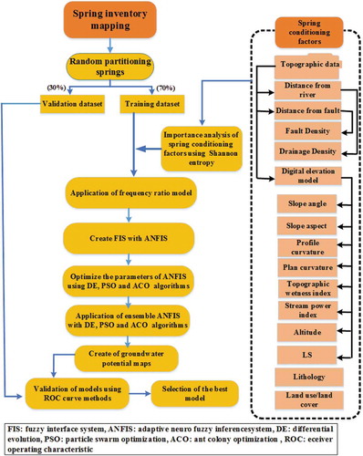
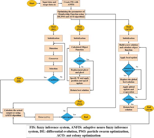
The methodological framework of this study, an ensemble of ANFIS and metaheuristic algorithms, comprises seven primary steps, shown in Fig. 2:

Step 1. Inventory mapping of springs in ArcGIS 10.2.

Step 2. Preparation of influencing factors in ArcGIS 10.2.

Step 3. Assessment of importance of factors using SE.

Step 4. Frequency ratio values for running the ANFIS model.

Step 5. Applying ensembles of ANFIS with metaheuristic algorithms (DE, PSO and ACO) in MATLAB software.

Step 6. Producing GPMs in ArcGIS 10.2.

Step 7. Validation of the GPMs in SPSS.

3.1 Historical spring locations

A groundwater spring inventory map shows the connection between the spatial distribution of springs and various geo-environmental factors. The spring inventory map, comprising 273 springs, was created from the national reporting of the Iranian Department of Water Resources Management (IDWRM). Comprehensive field surveys were carried out to determine spring locations using a handheld global positioning system (GPS; Fig. 1).

Figure 1. Study area of the Nahavand Plain, Iran, and location of springs

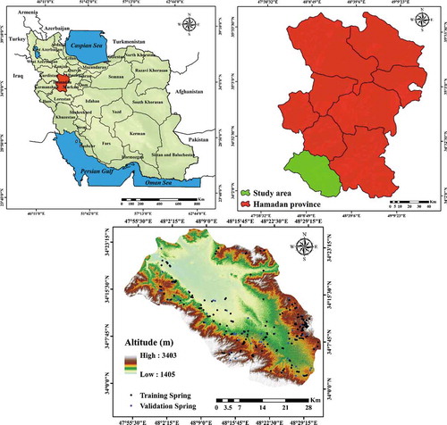
Figure 2. Flowchart of the methodology adopted in the study

3.2 Construction of training and testing dataset

The spring locations were split into two sub-sets, one for training and the other for the validation of groundwater mapping (Jaafari et al. 2014). Of the total number of springs in the study area (273), 70% (191 springs) were chosen for training and 30% (82 springs) for validation (Fig. 1). Since the spatial prediction of GPM is considered a binary classification, the same number of points were generated denoting the lack of a spring (non-spring) from the spring-free region and were divided into two sub-sets in a ratio of 70:30. Values of 1 and 0 were allocated to all spring and non-spring locations, denoting spring presence and absence, respectively (Bui et al. 2012; Pradhan et al. 2013). All 70% of both spring and non-spring locations were combined to build the training dataset, while 30% of both spring and non-spring locations were combined to construct the testing dataset. The training dataset was overlaid with 14 conditioning factors to extract attribute values and was used to train and modify the weights of parameters of the algorithms, while the testing dataset was used to evaluate the effectiveness of the algorithms.

3.3 Multicollinearity analysis

A multicollinearity test was applied after the selection of conditioning factors to evaluate the non-independence among conditioning factors that may happen owing to their elevated correlation in datasets (Dormann et al. 2013). Two techniques of tolerance (TOL) and variance inflation factor (VIF) are commonly used for identifying multicollinearity. Values of VIF > 5 or tolerance < 0.1 indicate potential multicollinearity in a dataset (if VIF > 10, there is high multicollinearity; Dormann et al. 2013). If VIF > 5, this indicates that two or more variables are interdependent and will cause an over-fitting error. Therefore, if the values of VIF or TOL exceed the threshold, that variable should be removed from use.

3.4 Groundwater-influencing factors

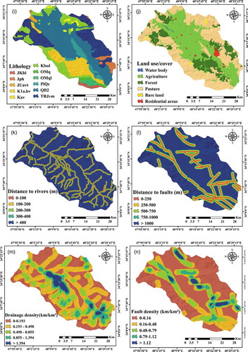
Fourteen factors were chosen in a GIS environment, based on a literature review, accessibility of information and features of the study area (Razandi et al. 2015, Rahmati et al. 2016, Naghibi et al. 2016). These factors are: altitude, slope angle, slope aspect, slope length, stream power index (SPI), topographic wetness index (TWI), plan curvature, profile curvature, land use/cover, lithology, distance from river, distance from fault, drainage density and fault density. Maps of of the factors are presented in Fig. 3. The quantile method was used for classification, as the data and histograms exhibited skewness.

The ASTER digital elevation model (DEM) was downloaded at a spatial resolution of 30 m × 30 m (https://gdex.cr.usgs.gov/gdex/), and topographic parameters of the study area, consisting of altitude, profile curvature, slope length, slope angle, TWI, plan curvature, SPI and slope aspect, were obtained from the DEM. Areas with varying altitudes had noticeable variations in climatic conditions, resulting in variations in vegetation and soil conditions and thus the potential for groundwater resources to be present (Aniya 1985, Park et al. 2017). Altitude was divided into five classes (<1800, 1800–2200, 2200–2600, 2600–3000 and >300 m asl; Fig. 3(a)). The slope angle has an important effect on runoff generation and therefore groundwater recharge. With increasing slope angle, runoff increases and the groundwater is recharged less (Vijith 2007, Mogaji et al. 2015). The slope angle was categorized into five classes: 0–5°, 5–15°, 15–25°, 25–35° and >35° (Fig. 3(b)). The slope aspect factors into the formation of groundwater in some hydrological processes, such as snow melting and direction of precipitation and physiographical trends, affecting the content of soil water (Park et al. 2017). This criterion was grouped into nine categories (Fig. 3(c)). The LS was calculated using Equation (1)(1) $LS={\left(\frac{B_s}{22.13}\right)}^{0.6}{\left(\frac{sin\alpha }{0.0896}\right)}^{1.3}$(1) , which is a composite of slope length (L) and slope angle (S) (Wischmeier and Smith 1978, Moore and Burch 1986), and was categorized into five groups: 0–5, 5–10, 10–15, 15–20 and >20 (Fig. 3(d)):

(1) $LS={\left(\frac{B_s}{22.13}\right)}^{0.6}{\left(\frac{sin\alpha }{0.0896}\right)}^{1.3}$(1)

Figure 3. Maps of groundwater conditioning factors: (a) altitude, (b) slope angle, (c) slope aspect, (d) LS, (e) SPI (stream power index), (f) TWI (topographic wetness index), (g) plan curvature, (h) profile curvature,(i) land use/cover, (j) lithology, (k) distance from river, (l) distance from fault, (m) drainage density and (n) fault density

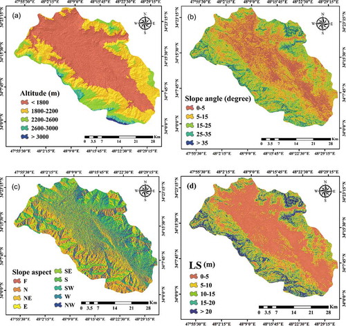
Figure 3. (Conitnued)

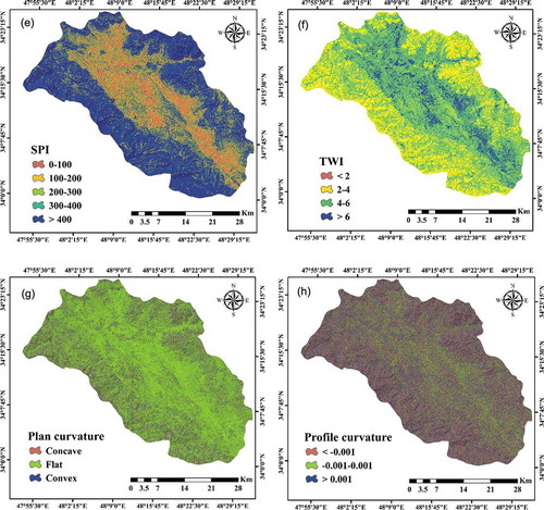
Figure 3. (Conitnued)

where α is the gradient of slope (degree) and $B_s$ is the particular catchment area (m²). The plain curvature is a shift along a contour line which directly controls the speed of water flow (Pradhan 2013). The curvature was categorized as convex, concave or flat (Fig. 3(e)). Another factor that affects groundwater occurrence is profile curvature, which is the slope downward along the flow line (Al-Abadi et al. 2016). A profile curvature map was prepared in SAGA-GIS and then categorized into three classes: < –0.05, –0.05 to 0.05 and >0.001 (Pham et al. 2017) (Fig. 3(f)). TWI is the flow accumulation at a certain point in the basin which tends to go to a lower surface (Moore et al. 1991). It was calculated directly from DEM as follows (Moore et al. 1991, Jaafari et al. 2014):

(2) $\mathrm{T}\mathrm{W}\mathrm{I}=ln\left(\frac{A_s}{tan\beta }\right)$(2)

where $A_s$ is the area of the cumulative upslope and β is the gradient of the slope. Finally, this factor was classified into four classes: <2, 2–4, 4–6 and >6 (Fig. 3(g)). SPI shows the erosive power of flow with a direct relation to slope and basin area and was calculated as follows (Moore et al. 1991):

(3) $\mathrm{S}\mathrm{P}\mathrm{I}=A_{s}tan\beta$(3)

where $A_s$ is the area of cumulative upslope and β is the gradient of the slope. SPI was divided into five classes: 0–100, 100–200, 200–300, 300–400 and >400 (Fig. 3(h)). The land use/cover map from Landsat-7 satellite imagery Enhanced Thematic Mapper Plus (ETM+) between 2016 and 2018 was obtained using the maximum likelihood algorithm at an accuracy of 91.4%. To this end, 850 training points obtained with the GPS were used to create the land use/cover map, 70% of which were used for training and 30% were used to test the map’s accuracy. Landsat image corrections were performed in ENVI 4.5. For geometric correction, 1:500 000-scale topographic maps were used. Six land use/cover classes in the study area were identified (agricultural, residential areas, bare land, pasture, forest and water body; Fig. 3(i)). Most of the study area is covered by pasture and agricultural crops. Due to interception because of a high amount of foliage and high permeability of soils, forest lands reduce flow velocity and splash erosion and thus, the effect of these regions on groundwater recharge is noticeable. Lithology and its associated characteristics play a major role in porosity, penetrability and groundwater flow concentration within rocks (Park et al. 2017). A lithology map of Nahavand was created from a 1:100 000-scale geological map obtained from the Iran Geology Survey (GSI) (1997) covering 13 lithological units (Table 1.; Fig. 3(j)). Rivers transfer the generated runoff and have a relationship with the permeability of lands: the higher the river flow, the lower the permeability of an area and vice versa (Koike et al. 1998, Dinesh Kumar et al. 2007). In this research, the rivers were delineated, using ArcHydro instruments, by a hill-shaded map generated from the DEM. The distance to the river was divided into five classes: <100, 100–200, 200–300, 300–400 and >400 m (Fig. 3(k)). Increasing interstices and fault densities play an important role in penetrating and transferring groundwater and so are important in extracting, protecting and dispersing contaminants (Prasad et al. 2008). Faults of the region were marked using a 1:100 000-scale geological map and, finally, the distances to faults were created and divided into five classes: <250, 250–500, 500–750, 750–1000 and >1000 m (Fig. 3(l)). The drainage density and fault density were split, respectively, into five groups: <0.193, 0.193–0.49, 0.498–0.85, 0.85–1.39 and >1.39 and <0.16, 0.16–0.48, 0.48–0.79, 0.79–1.12 and >1.12 (Fig. 3(m,n)).

3.5 Groundwater spring potential mapping using ensemble techniques

3.5.1 Analysis of importance of groundwater conditioning factors

In the SE method, variables are determined by their maximum effect on the occurrence of an event. In order to do zoning and mapping by entropy, the following equations were used (Bednarik et al. 2010, Constantin et al. 2011):

(4) $E_{ij}=\frac{\mathrm{F}\mathrm{R}}{{\sum }_{J=1}^{M_j}\mathrm{F}\mathrm{R}}$(4)

(5) $H_j=-{\sum }_{i=1}^{s_j}\left(E_{ij}\right){log}_2\left(E_{ij}\right),j=1,2,\dots ,n$(5)

(6) $H_{j\mathrm{m}\mathrm{a}\mathrm{x}}={log}_2{M}_j$(6)

(7) $I_j=\frac{H_{j\mathrm{m}\mathrm{a}\mathrm{x}}-H_j}{H_{j\mathrm{m}\mathrm{a}\mathrm{x}}}I=\left(0,1\right),j=1,2,..n$(7)

(8) $W_j=I_j\times \mathrm{F}\mathrm{R}$(8)

where FR is the frequency ratio value; $E_{ij}$ is the probability; $H_j$ and $H_{j\mathrm{m}\mathrm{a}\mathrm{x}}$ are entropy values and maximum entropy, respectively; $I_j$ is the information coefficient; $M_j$ is the number of classes; and $S_j$is the final weight of Shannon entropy for each criterion. The advantage of the entropy approach is that it considers the relationship between participating variables in preparing the groundwater potential map (Constantin et al. 2011).

3.5.2 FR model

A probabilistic connection between autonomous and dependent factors can be calculated using the FR model (Oh et al. 2011). The FR model’s advantages are that it is robust and easy to use (Khosravi et al. 2016a). The FR of each class of criterion was calculated using the following equation:

(9) $\mathrm{F}\mathrm{R}=\frac{\frac{A\left(i\right)}{{\sum }_{i=1}^{m}A\left(i\right)}}{\frac{C(\left(i\right)}{{\sum }_{i=1}^{n}C(\left(i\right)}}$(9)

In Equation (9)(9) $\mathrm{F}\mathrm{R}=\frac{\frac{A\left(i\right)}{{\sum }_{i=1}^{m}A\left(i\right)}}{\frac{C(\left(i\right)}{{\sum }_{i=1}^{n}C(\left(i\right)}}$(9) , A_(i) is the total value of pixels in each class of each criterion with spring locations; C_(i) is the total pixel value of each criterion; and m and n are, respectively, the number of classes per criterion and the total number of criteria. The FR model was applied to run the ANFIS model as an input.

3.5.3 ANFIS model

The ANFIS model structure is better than FIS for solving nonlinear issues (Wang and Elhag 2008). In ANFIS, the degree of membership, rules and functions of membership of the output were chosen in proportion to the input information (Wang and Elhag 2008). The ANFIS model structure consisted of five layers, as shown in Fig. 4.

The layers in the ANFIS model are characterized as follows: For Layer 1, each node contained adaptive variable nodes:

(10) $O_{1,i}=\mu A_i\left(x\right)$(10)

(11) $O_{1,i}=\mu B_i\left(y\right)$(11)

where the input nodes are x and y, the linguistic variables are A and B, and $\mu A_i\left(x\right)$ and $\mu B_i\left(y\right)$ are the node’s membership functions.

Layer 2 includes fixed nodes, referred to as Π in Fig. 4. Each node has a position as an operation “fuzzy AND,” which is used as the output layer for firing power calculation of the laws. Each node’s output is the result of all the node’s input signals:

(12) $O_{2,i}=W_i=\mu A_i\left(x\right)\mu B_i\left(y\right),i=1,2$(12)

Figure 4. ANFIS (adaptive neuro fuzzy inference system) model structure (Bui et al. 2012)

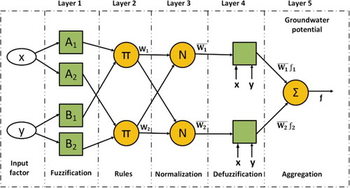
Figure 5. The process of implementing the ensemble models

where $W_i$is the node output.

Layer 3 includes the set of fixed nodes displayed in Fig. 4 as N. In fact, the nodes in this layer are the standardized outputs of Layer 2, known as the standard firepower:

(13) $O_{3,i}=\overline{w_l}=\frac{w_i}{w1+w2},i=1,2$(13)

A node function is connected with each node in Layer 4:

(14) $O_{4,i}=\overline{w_l}{f}_i=\overline{w_l}\left(p_{i}x+q_{i}y+r_i\right)$(14)

where $\overline{w_l}$is the Layer 3 standardized firepower; and$p_i$, $q_i$ and $r_i$are the parameters of the nodes. The resulting parameters were interpreted as parameters of this layer.

Layer 5 includes a single node given as ∑ which is the sum of the yield values of Layer 4 and displays the ANFIS model’s final outcome, given by:

(15) $O_{5,i}=\sum \overline{w_l}{f}_i=\sum w_i{f}_i/\sum w_i,i=1,2$(15)

In the training stage, the output values are brought nearer to the real values by changing the degree of membership parameters based on an acceptable error rate. Common training methods are error propagation and hybrid method (Termeh et al. 2018).

3.5.4 DE algorithm

In the DE algorithm there are three factors, namely mutation, crossover and selection, for reproducing the next optimal generation, and three parameters of control, namely scale factor (F), population size (NP) and crossover (Cr). The process of this algorithm is detailed below (Varadarajan and Swarup 2008).

3.5.4.1 Primary population generation

An initial population consisting of the NP member is generated randomly, so that each solution is in the space of answers. In any problem, with M-dimensional search space, the jth member structure can be written by (Storn and Price 1997):

(16) $X^i=\left(x_1^i,x_2^i,\dots .,x_m^i\right)$(16)

3.5.4.2 Mutation

For each member $X^i$ of the population, a new answer is generated for each t iteration using the following (Storn and Price 1995):

(17) $V_{i,G+1}=X_{r1,G}+F\ast \left(X_{r2,G}-X_{r3,G}\right)$(17)

where$r_1$, $r_2$, $r_3$ε [1, NP] are three unequal random integers. The coefficient F, called the scale factor, is between 0 and 2. This coefficient specifies the length of the mutation step.

3.5.4.3 Crossover

Here, one combination occurs between a mutant vector and a target member selected in the first stage, and the vector of measurement is generated. The basis of this combination is the Cr coefficient between 0 and 1 (Zheng et al. 2014). In this way, each component of this mutated vector is transferred with the probability of Cr to the candidate vector; otherwise, the equivalent component is replaced in the original vector. This operator is represented by the following (Storn and Price 1995):

(18) $u_{ji,G+1}=\left\{\begin{array}{c}{V}_{ji,G+1}if\left(\mathrm{r}\mathrm{a}\mathrm{n}\mathrm{d}\right)\le C_{r}orj=j_{\mathrm{r}\mathrm{a}\mathrm{n}\mathrm{d}}\\ X_{ji,G}otherwise\end{array}\right.$(18)

3.5.4.4 Selection

In this phase, the measurement vector obtained from the previous stage and the target group selected in the first phase is weighted according to the objective function, and if the vector of measurement has more value than the target member, it will be one of the members of the next generation. Otherwise, the target member becomes a member of the next generation. The choice between the vector of measurement and target member is given by the following (Zheng et al. 2014):

(19) $X_{ji,G+1}=\left\{\begin{array}{c}{u}_{ji,G+1}iff\left(u_{i,G+1}\right)\le f\left(X_{i,G}\right)\\ X_{ji,G}otherwise\end{array}\right.$(19)

3.5.5 PSO algorithm

The PSO algorithm, introduced by Kennedy and Eberhart (1995), produces strong results in the optimization of nonlinear problems. In this algorithm, an initial population of particles is formed, and then a target function for each particle is calculated (Shi and Eberhart 1999). The PSO algorithm is described mathematically as follows. The speed update was calculated using the following (Kennedy and Eberhart 1995):

(20) $V_{ij}\left(t+1\right)=W\times V_{ij}\left(t\right)+r_1\times {\mathrm{c}}_1\left(p_{ij}\left(t\right)-x_{ij}\left(t\right)\right)+r_2\times c_2\left({\mathrm{g}}_i\left(t\right)-x_{ij}\left(t\right)\right)$(20)

where $p_{ij}\left(t\right),$ $g_i\left(t\right),$ W,$c_1$,$c_2$,$r_1$ and$r_2$ are the best personal memory, the best collective memory, the inertial factor, the personal learning coefficient, the collective learning coefficient and the random numbers between (1 and 0), respectively. The new position of a particle is calculated using the following (Kennedy and Eberhart 1995):

(21) $X\left(t+1\right)=X\left(t\right)+V\left(t+1\right)$(21)

At each step after updating the speed for each particle, based on the prior position and the velocity of the new update, the new particle location is calculated.

3.5.6 ACO algorithm

The ACO is a suitable algorithm for finding approximate solutions for problems of combined optimization. In this method, artificial ants move on the problem chart and leave signs on it, like real ants leaving their mark on a path, which leads the ants that come next to provide better solutions to the problem (Huang et al. 2006). Also, in this way, it is possible to find the best route in a path by probability calculus-based methods. This technique, first introduced by Dorigo (1992), is inspired by ants’ behavior and finds a path between the nest and the food location.

In reality, ants randomly go back and forth to find food. Then they return to their nest, leaving a pheromone trace behind them. Other ants finding the path sometimes leave, wander or follow it. If they reach the food, they go home and leave another trace behind them. In other words, they reinforce the previous path. The aim of the ACO algorithm is to imitate this behavior of artificial ants moving on the graph (Dorigo and Blum 2005). In each iteration, ants use a probability transfer function based on Equation (22)(22) $P_{ij}^k(t)=\{\begin{array}{l}\frac{{\tau }_{ij}^{\alpha }\left(t\right)*{\eta }_{ij}^{\beta }\left(t\right)}{{\displaystyle {\sum }_{u{N}_i^k}{\tau }_{iu}^{\alpha }\left(t\right)*{\eta }_{iu}^{\beta }\left(t\right)}}\\ 0j\notin N_i^k\end{array}$(22) (Beckers et al. 1992) to transfer from the current position to the next and calculate the probability of transfer to all subsequent points (points that have not yet been):

(22) $P_{ij}^k(t)=\{\begin{array}{l}\frac{{\tau }_{ij}^{\alpha }\left(t\right)*{\eta }_{ij}^{\beta }\left(t\right)}{{\displaystyle {\sum }_{u{N}_i^k}{\tau }_{iu}^{\alpha }\left(t\right)*{\eta }_{iu}^{\beta }\left(t\right)}}\\ 0j\notin N_i^k\end{array}$(22)

where ${\mathrm{P}}_{\mathrm{i}\mathrm{j}}^{\mathrm{k}}$(t) is the probability of ant k moving from point i to point j in the t iteration; ${\mathrm{T}}_{ij}^{\alpha }$ is the density of pheromone corresponding to connection (i,j);${\hspace{0.17em}}_{ij}^{\beta }\left(\mathrm{t}\right)$ shows the transition optimality from point i to point j and is known as exploratory information, which in this case is proportionate to the inverse distance between two points; $N_i^k$ is the total number of points not yet visited by ant k, and the ant is allowed to pass by them; and Α and β are constant indices representing the importance of pheromones and exploratory information (Beckers et al. 1992). After the probability has been calculated, a point with high probability is randomly selected by an ant for the next move. When an ant completes its route, the cost of the route is evaluated by the objective function. In each iteration, when all ants complete their paths, pheromones are updated. Updating pheromones is done by the following (Beckers et al. 1992):

(23) ${\tau }_{ij}(t+1)=1=(1-\rho ){\tau }_{ij}(t)+{\sum }_{k=1}^{N\mathrm{a}\mathrm{n}t}n{\tau }_{ij}^k$(23)

where ρ is the evaporation coefficient; N is the number of all ants passing between i and j; and ${\tau }_{ij}^k$ is calculated by the following (Beckers et al. 1992):

(24) $n{\tau }_{ij}^k=\left\{\begin{array}{c}\frac{Q}{{\mathrm{L}}_{\mathrm{k}}}\mathrm{i}\mathrm{f}\left(\mathrm{i},\mathrm{j}\right)\in {\mathrm{x}}_{}^{\mathrm{k}}\left(\mathrm{t}\right)\\ \\ 0\mathrm{o}\mathrm{t}\mathrm{h}\mathrm{e}\mathrm{r}\mathrm{w}\mathrm{i}\mathrm{s}\mathrm{e}\end{array}\right.$(24)

In this equation, $L_k$ is the length of the path made by ant k in the previous step, Q is a positive constant and $x_k\left(t\right)$ is the total of all edges visited by ant k (Beckers et al. 1992).

3.5.7 Ensemble of ANFIS and metaheuristic algorithms

To minimize the error between the ANFIS output (predicted) and the actual output (observed), the learning algorithm of ANFIS seeks to determine the preceding and consequent parameters. Referring to the framework of ANFIS (Fig. 4), the general output can be described as a linear combination of consequent parameters as follows: The technique of gradient descent is the classic algorithm for updating the predicate parameters. However, the greatest learning rate in the gradient descent technique is difficult to identify, and the method-based convergence of predicate parameters is slow. As metaheuristic algorithms, PSO, DE and ACO have been used in this research to enhance the outcomes of the ANFIS model and also to fine-tune the parameters of membership functions (Mahapatra et al. 2015, Razavi-Termeh et al. 2020a). The objective functions of metaheuristic algorithms are given by the following (Mahapatra et al. 2015):

(25) $e=t-y$(25)

(26) $\mathrm{R}\mathrm{M}\mathrm{S}\mathrm{E}=\sqrt{\mathrm{M}\mathrm{e}\mathrm{a}\mathrm{n}\left(e^2\right)}$(26)

(27) $\mathrm{O}\mathrm{b}\mathrm{j}\mathrm{e}\mathrm{c}\mathrm{t}\mathrm{i}\mathrm{v}\mathrm{e}\mathrm{f}\mathrm{u}\mathrm{n}\mathrm{c}\mathrm{t}\mathrm{i}\mathrm{o}\mathrm{n}=\mathrm{m}\mathrm{i}\mathrm{n}(\mathrm{R}\mathrm{M}\mathrm{S}\mathrm{E})$(27)

where t, y and e are the target information, the input information function, and the fuzzy system with optimized values and the error function value to be minimized, respectively. To evaluate model efficiency, root mean squared error (RMSE) was used. In the first phase of ensemble models, after entering the target and training data, the fuzzy interface system (FIS) was created by ANFIS. In the second phase, after initialization parameters in DE, PSO and ACO algorithms, FIS was optimized by these algorithms until the termination condition was seized. Figure 5 shows the flowchart of the proposed technique.

3.5.8 Model validation

The three maps produced in this study were validated using the receiver operating characteristic (ROC) curve. For any possible cutoff error, the ROC curve is a graphical display of the balance between negative and positive error rates, and the area under the ROC curve (AUC) quantitatively demonstrates the model’s predictive capacity (Bui et al. 2012, Razavi-Termeh et al. 2019). The test dataset (prediction rate) was used to assess the prepared maps and their accuracy. The training and testing datasets represent the suitability of the built algorithms and how good the algorithms are for GPM, respectively. So, the performance of an algorithm should be assessed with data not used in the training phase (Jaafari et al. 2019). The true positive and false positive values of the graph were calculated according to the following equations (Constantin et al. 2011, Razavi-Termeh et al. 2020b):

(28) $X=1-\left[\frac{\mathrm{T}\mathrm{N}}{\mathrm{T}\mathrm{N}+\mathrm{F}\mathrm{P}}\right]$(28)

(29) $Y=\left[\frac{\mathrm{T}\mathrm{P}}{\mathrm{T}\mathrm{P}+\mathrm{F}\mathrm{N}}\right]$(29)

where TP, TN, FP and FN represent the true positive, true negative, false positive and false negative values, respectively. The ideal algorithm has the highest AUC, with its range varying from 0.5 to 1 (Zhu and Wang 2009). Also, the prediction performance of the algorithms was classified based on AUC as poor (low), moderate, good, very good and excellent for values of 0.5–0.6, 0.6–0.7, 0.7–0.8, 0.8–0.9 and 0.9–1, respectively.

4 Results

4.1 Multicollinearity diagnosis

Table 2 summarizes the results of assessment of the 14 autonomous multicollinearity factors. These results show that the TOL and VIF were >0.1 and <10, respectively, for all factors used. This shows that there was no issue of multicollinearity among the independent factors used.

Table 1. Lithological characteristics of the study area

Code	Lithology	Geological age
Qft2	Low-level piedmont fan	Cenozoic
TRJvm	Meta-volcanic phyllites, slate and meta-limestone	Mesozoic
Klsol	Gray, thick-bedded to massive orbitolina limestone	Mesozoic
Jph	Phyllite-slate and meta-sandstone	Mesozoic
Kav	Andesitic volcanic	Mesozoic
JUavt	Andesitic volcanic tuff	Mesozoic
K1a.bv	Andesitic and basaltic volcanic rocks	Mesozoic
PlQc	Fluvial conglomerate, piedmont conglomerate and sandstone	Cenozoic
OMq	Limestone, sandstone and sandy marl	Cenozoic
OMql	Massive thick-bedded reefal limestone	Cenozoic
JKbl	Gray, thick-bedded, fetid limestone	Mesozoic

Table 2. Multicollinearity diagnostic indices for independent variables: TWI: Topographic Wetness Index, SPI: Stream Power Index, VIF: variance inflation factor

Factor	Tolerance	VIF
Aspect	0.945	1.058
Altitude	0.764	1.309
Fault density	0.440	2.275
Drainage density	0.885	1.130
Distance from fault	0.446	2.241
Lithology	0.601	1.664
Land use/cover	0.836	1.196
LS	0.706	1.416
Plan curvature	0.722	1.385
Profile curvature	0.749	1.335
Distance from river	0.890	1.124
Slope angle	0.691	1.447
SPI	0.698	1.433
TWI	0.791	1.264

4.2 Analysis of relative importance of groundwater conditioning factors

The results of the SE approach are summarized in Table 3. The higher the SE coefficient, the more important the factor. According to the coefficients from the SE model, the factor having the greatest effect on groundwater occurrence in the Nahavand Plain is land use/cover (0.673), followed by lithology (0.281), altitude (0.237), slope angle (0.187), slope length (0.142), distance from river (0.099), TWI (0.097), fault density (0.062), distance from fault (0.052), plan curvature (0.048), drainage density (0.044), SPI (0.04), slope aspect (0.016) and profile curvature (0.0098).

Table 3. Results of the frequency ratio (FR) and Shannon entropy (SE) models: TWI: Topographic Wetness Index, SPI: Stream Power Index

Class	No. of pixels in domain	No. of springs	FR	$E_{ij}$	$H_j$	$H_{j\mathrm{m}\mathrm{a}\mathrm{x}}$	$I_j$	$W_j$
Altitude (m)
<1800	103591	83	0.807	0.285	1.3432	2.3219	0.421	0.237
1800–2200	606363	100	1.66	0.588
2200–2600	226084	8	0.356	0.126
2600–3000	47751	0	0	0
>3000	9422	0	0	0
Slope angle
0–5	562265	48	0.86	0.273	1.6311	2.3219	0.297	0.187
5–15	743319	122	1.654	0.525
15–25	388464	8	0.467	0.148
25–35	182113	3	0.166	0.0527
>35	49376	0	0	0
Slope aspect
Flat	18980	2	1.062	0.118	3.1168	3.1699	0.016	0.016
North	284628	33	1.16	0.129
Northeast	273826	26	0.957	0.106
East	213404	17	0.803	0.089
Southeast	209002	10	0.482	0.053
South	239626	21	0.883	0.098
Southwest	234945	30	1.287	0.143
West	217631	25	1.158	0.129
Northwest	233495	27	1.165	0.13
Plan curvature
Concave	296191	38	1.29	0.439	1.5044	1.5850	0.05	0.048
Flat	118960	129	1.093	0.372
Convex	439744	24	0.55	0.187
Profile curvature
<–0.05	622201	48	0.777	0.264	1.5676	1.5850	0.01	0.0098
–0.05–0.05	980118	110	1.131	0.384
>0.05	323218	33	1.029	0.35
LS
0–5	996559	97	0.981	0.232	1.9270	2.3219	0.17	0.142
5–10	362193	67	1.86	0.441
10–15	241919	16	0.66	0.156
15–20	158183	10	0.637	0.151
>20	166683	1	0.06	0.0142
SPI
<100	302244	13	0.433	0.121	2.1897	2.3219	0.057	0.04
100–200	202740	11	0.546	0.153
200–300	139675	7	0.505	0.142
300–400	105860	8	0.761	0.214
>400	117502	152	1.304	0.367
TWI
<2	57	0	0	0	1.2157	2	0.392	0.097
2–4	651584	18	0.278	0.122
4–6	107462	164	1.538	0.677
>6	199276	9	0.455	0.2
Distance from fault
<250	176981	31	1.76	0.242	2.2379	2.3219	0.0361	0.0524
250–500	166107	33	2.003	0.275
500–750	154792	19	1.237	0.17
750–1000	138860	22	1.59	0.218
>1000	128936	86	0.672	0.092
Distance from river
<100	137073	35	2.574	0.4	2.1398	2.3219	0.078	0.099
100–200	124785	16	1.293	0.203
200–300	132883	10	0.758	0.119
300–400	117362	10	0.859	0.135
>400	141400	120	0.855	0.134
Fault density
<0.16	105621	62	0.591	0.09	2.2108	2.3219	0.047	0.062
0.16–0.48	376315	48	1.28	0.195
0.48–0.79	310957	50	1.62	0.247
0.79–1.12	122709	25	2.05	0.312
>1.12	59912	6	1.009	0.154
Drainage density
<0.193	599494	52	0.874	0.177	2.2181	2.3219	0.044	0.044
0.193–0.498	718214	61	0.856	0.174
0.498–0.855	358352	55	1.547	0.314
0.855–1.394	162626	19	1.178	0.239
>1.394	87417	4	0.461	0.093
Lithology
Qft2	703177	42	0.602	0.061	2.3677	3.4594	0.315	0.281
TRJvm	430982	68	1.591	0.161
Klsol	296646	10	0.339	0.034
Jph	51947	21	4.076	0.414
Kav	21294	0	0	0
Juavt	12315	0	0	0
K1a.bv	239238	40	1.68	0.17
PlQc	86878	8	0.928	0.0944
OMq	23574	0	0	0
OMql	32799	2	0.614	0.062
JKbl	27251	0	0	0
Land use/land cover
Residential areas	23157	3	1.3	0.25	1.8064	2.5850	0.7786	0.673
Pasture	886843	45	0.511	0.098
Agriculture	691089	70	1.021	0.196
Forest	312056	73	2.359	0.454
Water body	2867	0	0	0
Bare land	10089	0	0	0

4.3 Results of the FR algorithm

Table 3 summarizes the results of the FR algorithm. The outcome of the altitude factor showed that the maximum FR value was in the range 1800–2200 m (1.66). The FR value was the highest for the 5–15° class in the slope angle (1.654). The results indicate that the highest FR value was observed in southwest-facing areas (1.287), while concave areas had maximum FR = 1.29, followed by flat (1.093) in the plan curvature. The maximum FR value for the profile curvature was observed for the class –0.05 to 0.05 (1.13). For the slope length factor, the lengths of 5–10 m and 0–5 m had high potential for groundwater spring occurrence, with FR values of 1.86 and 0.986, respectively. The results for the SPI factor show that values >400 gave the maximum FR (1.304). The results for TWI indicate that values of 4–6 had a higher impact on spring occurrence (1.53), as about 85% of the springs occurred in this category. For the factor distance from fault, the classes 250–500 and >1000 m had, respectively, the highest (2.003) and lowest (0.67) correlation with spring occurrence in the Nahavand Plain. In the case of the river factor, the FR values showed a declining trend when the river range increased, and the largest FR value (2.574) was found for the river class 0–100 m. The results of the fault density factor show that the range 0.79–1.12 km/km² had the highest FR value (2.05), whereas for the drainage density factor, the range of 0.498–0.855 km/km² had the maximum FR (1.547). For the lithology factor, the Jph unit (phyllite-slate and meta-sandstone) had the highest FR value (4.076 for Jph), showing the greatest likelihood of a spring incidence. The highest FR values for the land use/cover factor were for forest (2.359), followed by residential areas (1.3). This shows that the forest land use had the greatest likelihood of the occurrence of springs. Vegetation affects penetration, so the highest permeability occurs in forest areas.

4.4 ANFIS ensemble models and model performance assessment

An ensemble of ANFIS and three metaheuristic algorithms (ANFIS-DE, ANFIS-PSO and ANFIS-ACO) was constructed and implemented in MATLAB 8.0 software. For algorithm building, all 14 conditioning factors and the training dataset were used. The first step in algorithm construction was the determination of the rate for each class of conditioning factor by the FR algorithm (FR values were normalized or rescaled to the range 0–1). In the second step, the training datasets “with spring,” which were assigned a value of 1, and “non-spring,” which were assigned a value of 0, were used as an output. In the third step, modelling accuracy was calculated. The predictive power of these three ensemble algorithms (models) with the training dataset as target, and estimated spring pixels as output (in the training phase) and the test dataset (in the validation phase), is shown in Figs 6 and 7, respectively. The controlled parameters in each metaheuristic algorithm are summarized in Table 4. The parameters used in the ANFIS model design are presented in Table 5.

Table 4. Parameters used in an ensemble approach employing the metaheuristic algorithms: differential evolution (DE), particle swarm optimization (PSO) and ant colony optimization (ACO)

PSO	ACO	DE
Population = 100	Population = 100	Population = 100
Iteration = 1000	Iteration = 1000	Iteration = 1000
W = 1	${\tau }_0=1$	Lower Bound of Scaling Factor = 0.2
C1 = 1	$\alpha =1$	Upper Bound of Scaling Factor = 0.8
C2 = 2	$\beta =2$	Crossover Probability = 0.1
	$\rho =0.1$

Table 5. Parameters used in the adaptive neuro fuzzy inference system (ANFIS) model: FIS: fuzzy inference system

Parameter	Value
FIS generation approach	FCM (Fuzzy c-means)
Optimization method	Hybrid
Number of clusters	15
Partition matrix exponent	2
Number of iteration	200
Minimum improvement	1*e^−5
Number of epochs	200
Initial step size	0.01
Step size decrease rate	0.9
Step size increase rate	1.1

The RMSE was used to evaluate the accuracy of the training and testing datasets in the ensemble model. A lower RMSE for the training data indicated better prediction power of a built model. The ANFIS-DE model had the lowest RMSE (0.301) among the ANFIS ensemble models, followed by the ANFIS-PSO (0.396) and ANFIS-ACO (0.400) models. The ANFIS-DE model had the highest RMSE value during the validation phase (0.505), followed by the ANFIS-PSO (0.428) and ANFIS-ACO (0.424) models, showing that ANFIS-ACO performed better in the testing phase than the other two models did. According to the error diagram (Fig. 6(c)Fig. 7), the ANFIS-DE model followed a normal distribution with respect to the two other models.

Figure 6. Training dataset: ANFIS-DE (І), ANFIS-PSO (II), ANFIS-ACO (III) models: (a) target and output values, (b) MSE and RMSE values and (c) frequency errors

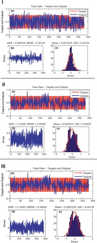
Figure 7. Testing dataset: ANFIS-DE (І), ANFIS-PSO (II), ANFIS-ACO (III) models: (a) target and output values, (b) MSE and RMSE values and (c) frequency errors

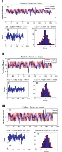
Figure 8. Convergence graphs of the objective function

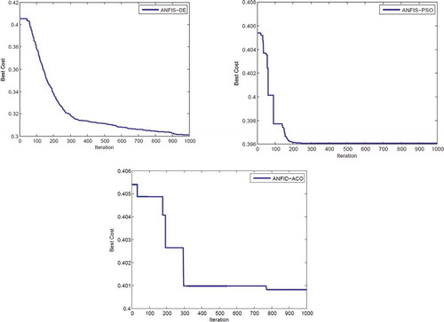
Figure 9. Convergence time graph of combined models

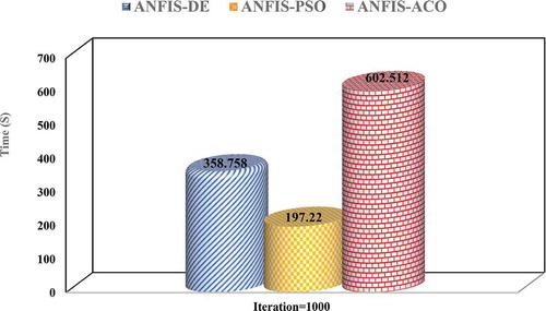
Figure 10. Groundwater potential map (GPM) of the study area made with (a) the ANFIS-DE model, (b) the ANFIS-PSO model and (c) the ANFIS-ACO model

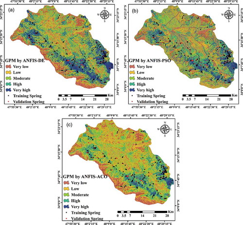
Figure 11. Results of ROC (receiver operating characteristic) curves for the ensemble models

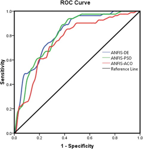
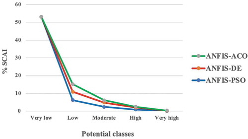
Figure 12. Seed cell area index (SCAI) for the three hybrid models in the Nahavand Plain, Iran

After implementing the ensemble models, a convergence graph of the objective function for each algorithm with 1000 iterations was constructed, as shown in Fig. 8. Considering that the objective function was minimization, the ANFIS-DE model, with a value of 0.301, had the best convergence in adjusting the parameters of ANFIS, followed by ANFIS-PSO and ANFIS-ACO, with values of 0.396 and 0.400, respectively. Based on the results of the convergence diagram, the ANFIS-PSO model in iteration 230, the ANFIS-ACO model in iteration 780 and the ANFIS-DE model in iteration 960 reached convergence. The results show that the ANFIS-PSO model was more convergent than the other two models. The timing of implementation of the three models is shown in Fig. 9. The execution times of the ANFIS-PSO, ANFIS-DE and ANFIS-ACO models were 197.22, 358.758 and 602.512 s, respectively. The ANFIS-PSO model had a faster convergence time and less running time than the other two models.

4.5 GPMs produced using ANFIS ensemble models

The ANFIS hybrid models with DE, PSO and ACO algorithms were constructed, using the training dataset and standardized FR values. Then, the built models were used for the prediction of the spring index (SI) which was assigned to the study area and, finally, GPMs were produced from the SI classification. The three GPMs, constructed using GIS based on the SI data for each algorithm, were divided into five classes, namely very low potential, low potential, moderate potential, high potential and very high potential, based on the quantile classification scheme shown in Fig. 10(a–c).

4.6 Validation of GPMs

Prediction curve results are shown in Fig. 11 and Table 6. In this study, the GPM gave AUC values of 0.8 or higher for the ANFIS-DE (0.816) and ANFIS-PSO (0.809) models, indicating very good predictive potential for both models, with the performance of the ANFIS-DE model being better than that of both the ANFIS-PSO model and the ANFIS-ACO (0.758; good) model.

Table 6. Results of area under curve (AUC) for the ensemble models

Model	Area	Standard error	Asymptotic Sig	Asymptotic 95% confidence interval
				Lower bound	Upper bound
ANFIS-DE	0.816	0.033	0.000	0.752	0.881
ANFIS-PSO	0.809	0.034	0.000	0.743	0.876
ANFIS-ACO	0.758	0.038	0.000	0.683	0.832

4.7 Percentage of GPM classes of different models

Table 7 shows the percentage of groundwater potential for each model. According to the ANFIS-DE model, a very high potential area covered 5.4% of the total area. It should be noted that two other models underestimated the high and very high potential groundwater areas.

Table 7. Spring distribution in predicted groundwater potential zones. SCAI: seed cell area index

Model	Groundwater potential zone	% Area of predicted zone	% Observed spring per zone	SCAI
ANFIS-DE	Very low	29.48	0	None
	Low	24.46	5.2	4.7
	Moderate	19.9	8.3	2.39
	High	20.76	17.8	1.16
	Very high	5.4	68.7	0.07
ANFIS-PSO	Very low	27.6	0.52	53.07
	Low	26.083	4.18	6.23
	Moderate	20.209	8.37	2.41
	High	20.208	21.98	0.919
	Very high	5.9	64.95	0.09
ANFIS-ACO	Very low	18.12	0	None
	Low	30.82	7.3	4.22
	Moderate	28.49	20.9	1.36
	High	16.5	41.8	0.394
	Very high	6.07	29.8	0.2

The seed cell area index (SCAI) was used to reassure the reliability of each class according to the following (Süzen and Doyuran 2004; Khosravi et al. 2016b):

(30) $\mathrm{S}\mathrm{C}\mathrm{A}\mathrm{I}=\frac{\mathrm{A}\mathrm{r}\mathrm{e}\mathrm{a}\mathrm{e}\mathrm{x}\mathrm{t}\mathrm{e}\mathrm{n}\mathrm{t}\mathrm{o}\mathrm{f}\mathrm{p}\mathrm{o}\mathrm{t}\mathrm{e}\mathrm{n}\mathrm{t}\mathrm{i}\mathrm{a}\mathrm{l}\mathrm{c}\mathrm{l}\mathrm{a}\mathrm{s}\mathrm{s}\left(\mathrm{\%}\right)}{\mathrm{S}\mathrm{p}\mathrm{r}\mathrm{i}\mathrm{n}\mathrm{g}\mathrm{i}\mathrm{n}\mathrm{e}\mathrm{a}\mathrm{c}\mathrm{h}\mathrm{p}\mathrm{o}\mathrm{t}\mathrm{e}\mathrm{n}\mathrm{t}\mathrm{i}\mathrm{a}\mathrm{l}\mathrm{c}\mathrm{l}\mathrm{a}\mathrm{s}\mathrm{s}\left(\mathrm{\%}\right)}$(30)

From the SCAI index, it is expected that very low and low potential classes would have higher SCAI values, and high and very high potential classes would have lower SCAI values (Khosravi et al. 2016b). The SCAI index results shown in Table 7 and Fig. 12 indicate a logical reliability between potential classes.

5 Discussion

Groundwater is the world’s most vital natural resource, which supplies water in arid and semi-arid countries. Recognition of groundwater resources can be helpful for sustainable management of groundwater. So far, several methods have been developed to provide groundwater potential maps using statistical methods, such as FR, WOE, EBF and LR. Recently, machine learning methods, due to their flexible and nonlinear structure, have been widely used for environmental modelling. There are also several other benefits of machine learning algorithms over traditional statistical modelling. Statistical modelling is all about getting a simple formulation of a frontier in a classification model problem. Statistical modelling operates on a variety of assumptions, but machine learning algorithms are spared from most of these assumptions. It is also not necessary to define the distribution of dependent or independent variables for machine learning algorithms. Machine learning is useful for a large number of properties and a large number of observations. However, for less information with fewer characteristics, statistical modelling is usually implemented, or such models end up over-fitting. The philosophical approach to model building presents an extra distinction worth noting between machine learning and statistical models. Statistical models almost always suppose that there is one fundamental “information-generating model,” and excellent practice requires the analyst to build a model using inputs that have a logical foundation to relate to the independent variable somehow. Machine learning, on the other hand, essentially does not require a priori beliefs about the nature of the true underlying relationships, and does not even necessarily expect only one best model to be discovered.

The ANFIS model, a hybrid of the ANN and FL models, is one of the machine learning algorithms widely used by researchers and has demonstrated its accuracy in the modelling of natural phenomena, such as landslide modelling (Polykretis et al. 2015), flood susceptibility mapping (Termeh et al. 2018) and groundwater potential mapping (Khosravi et al. 2018). The ANFIS model benefits from both ANN and FL models, but the primary disadvantage of this model is that the membership function parameters are not properly adjusted. In this study, DE, PSO and ACO algorithms were used to adjust these parameters and to determine optimal weights. The outcomes of the RMSE calculations indicate that the ANFIS-DE model was more accurate in the training phase, or had better goodness of fit, compared to the two other models, but in the testing phase the ANFIS-ACO had better prediction power. This shows that ANFIS-DE, due to over-fitting, had a good fit, but did not have the highest prediction power in the testing phase or generalization. Also, the results of the ROC curve method indicate that the ANFIS-DE algorithm had a higher accuracy in the prediction of GPM compared to the two other algorithms. The RMSE is based on error evaluation; therefore, it is not as suitable for comparison with the ROC curve, but the models should be applied holistically in accordance with their ability. Therefore, for contrast, both success and predictive ROC curves based on TP, TN, FP and FN were more accurate than RMSE (Termeh et al. 2018). Also, according to the convergence diagram, the DE algorithm had a higher accuracy than the PSO and ACO algorithms in setting parameters of the membership function.

A reason for DE and PSO algorithms being superior to the ACO algorithm was their memory function, such that all particles retained an understanding of useful alternatives. In other words, each particle benefited from its previous data, whereas in the ACO algorithm there was no such attribute and the previous knowledge was suddenly lost when the population changed. Also, in the DE and PSO algorithms, each member of a population shared its information with other particles, which made it more precise to search for all particles, but such an ability did not exist in the ACO algorithm. Other advantages of the DE and PSO algorithms were their high convergence rate, simplicity and strength. The PSO algorithm suffered from some weaknesses, including hasty convergence, getting stuck in the optimal locale and lack of local search. The main benefits of the DE algorithm were its ability to manage non-differentiable, nonlinear and multimodal object functions, as well as its ability to manage computationally intensive object functions. Having such operators as selection, crossover and mutation as well as local search, the DE algorithm was more accurate in adjusting the parameters of ANFIS than were the other algorithms. Due to the large number of parameters and using the roulette wheel approach in the initial selection of population members, implementation of the ACO algorithm was difficult and slow. In addition, a lack of local searches was another reason for the lower accuracy of this algorithm compared to the two other algorithms.

6 Conclusion

Identification and protection of groundwater are the most effective approaches to sustainable management of groundwater. While there are several methods for the identification of groundwater potential occurrence, due to the nonlinear and complex structure of natural phenomena, machine learning is suitable for environmental modelling. Although ANFIS is one of the most powerful machine learning algorithms and its performance has been proven in the modelling of natural phenomena, it is not able to adjust the membership function parameters. In this study, the DE, PSO and ACO algorithms were used to overcome this problem.

According to the SE model, the four most important factors influencing groundwater spring occurrence were land use, lithology, altitude and slope angle, while the least influential factor was related to profile curvature. The results of FR modelling revealed that springs occurred at an altitude of 1800–2000 m, a slope angle of 5–15°, a southwesterly aspect, SPI > 400, TWI = 4–6, Jph lithology, forest lands, 100–200 m distance from a river and 250–500 m distance from a fault.

The results of convergence of objective function show that the DE algorithm had the best value, followed by PSO and ACO. Also, according to the ROC curve approach, the ANFIS-DE had the highest prediction capability in GPM. The DE metaheuristic algorithm has some advantages in comparison to the two other models, including the capacity to manage non-differentiable, nonlinear and multimodal cost functions and the parallel capacity to manage extensive object functions for GPM computation. The GPMs obtained by the ANFIS-DE model illustrate that 26% of the Nahavand Plain, situated in the southern part of the study region, is covered by areas of high and very high groundwater spring potential.

Since no study has been done in preparing GPMs in the Nahavand Plain, this study can clarify the potential status of groundwater in Nahavand. It can also be stated that these maps can play a significant role in future decision-making, management and exploitation of groundwater in the region.

Disclosure statement

No potential conflict of interest was reported by the authors.

Additional information

Funding

This research was supported by MSIT (Ministry of Science and ICT), Korea, under the ITRC (Information Technology Research Center) support program [IITP-2020-2016-0-00312] supervised by the IITP (Institute for Information & communications Technology Planning & Evaluation).

References

- Adiat, K., Nawawi, M., and Abdullah, K., 2012. Assessing the accuracy of GIS-based elementary multi criteria decision analysis as a spatial prediction tool–a case of predicting potential zones of sustainable groundwater resources. Journal of Hydrology, 440, 75–89. doi:10.1016/j.jhydrol.2012.03.028
- Al-Abadi, A.M., Al-Temmeme, A.A., and Al-Ghanimy, M.A., 2016. A GIS-based combining of frequency ratio and index of entropy approaches for mapping groundwater availability zones at Badra–Al Al-Gharbi–Teeb areas, Iraq. Sustainable Water Resources Management, 2 (3), 265–283. doi:10.1007/s40899-016-0056-5
- Aniya, M., 1985. Landslide-susceptibility mapping in the Amahata river basin, Japan. Annals of the Association of American Geographers, 75 (1), 102–114.
- Arkoprovo, B., Adarsa, J., and Prakash, S.S., 2012. Delineation of groundwater potential zones using satellite remote sensing and geographic information system techniques: a case study from Ganjam district. Orissa, India. Research Journal of Recent Sciences, 1(9), 59–66.
- Bandyopadhyay, S., et al., 2007. Harnessing earth observation (EO) capabilities in hydrogeology: an Indian perspective. Hydrogeology Journal, 15 (1), 155–158. doi:10.1007/s10040-006-0122-4
- Banks, D., Robins, N., and Robins, N., 2002. An introduction to groundwater in crystalline bedrock. Trondheim: Geological survey of Norway. ISBN 82-7386-100-1.
- Beckers, R., Deneubourg, J-L. and Gross S. 1992. Trails and U-turns in the selection of a path by the ant Lasius niger. Journal of Theoretical Biology, 159 (4), 397–415. doi:10.1016/S0022-5193(05)80686-1
- Bednarik, M., et al., 2010. Landslide susceptibility assessment of the Kraľovany–Liptovský Mikuláš railway case study. Physics and Chemistry of the Earth, Parts A/B/C, 35 (3–5), 162–171. doi:10.1016/j.pce.2009.12.002
- Bui, D.T., et al., 2012. Landslide susceptibility mapping at Hoa Binh province (Vietnam) using an adaptive neuro-fuzzy inference system and GIS. Computers & Geosciences, 45, 199–211. doi:10.1016/j.cageo.2011.10.031
- Bui, D.T., et al., 2017. Spatial prediction of rainfall-induced landslides for the Lao Cai area (Vietnam) using a hybrid intelligent approach of least squares support vector machines inference model and artificial bee colony optimization. Landslides, 14 (2), 447–458.
- Chau, K., Wu, C., and Li, Y., 2005. Comparison of several flood forecasting models in Yangtze River. Journal of Hydrologic Engineering, 10 (6), 485–491. doi:10.1061/(ASCE)1084-0699(2005)10:6(485)
- Chen, W., et al., 2019. Spatial prediction of groundwater potentiality using ANFIS ensembled with teaching-learning-based and biogeography-based optimization. Journal of Hydrology, 572, 435–448. doi:10.1016/j.jhydrol.2019.03.013
- Chen, W., Panahi, M., and Pourghasemi, H.R., 2017. Performance evaluation of GIS-based new ensemble data mining techniques of adaptive neuro-fuzzy inference system (ANFIS) with genetic algorithm (GA), differential evolution (DE), and particle swarm optimization (PSO) for landslide spatial modelling. Catena, 157, 310–324. doi:10.1016/j.catena.2017.05.034
- Chowdhury, A., et al., 2009. Integrated remote sensing and GIS‐based approach for assessing groundwater potential in West Medinipur district, West Bengal, India. International Journal of Remote Sensing, 30 (1), 231–250. doi:10.1080/01431160802270131
- Clapcott, J., Goodwin, E., and Snelder, T., 2013. Predictive models of benthic macro-invertebrate metrics. Prepared for Ministry for the Environment. Cawthron Report No. 2301. 35 p. plus appendices.
- Constantin, M., et al., 2011. Landslide susceptibility assessment using the bivariate statistical analysis and the index of entropy in the Sibiciu Basin (Romania). Environmental Earth Sciences, 63 (2), 397–406. doi:10.1007/s12665-010-0724-y
- Corsini, A., Cervi, F., and Ronchetti, F., 2009. Weight of evidence and artificial neural networks for potential groundwater spring mapping: an application to the Mt. Modino area (Northern Apennines Italy). Geomorphology, 111 (1–2), 79–87. doi:10.1016/j.geomorph.2008.03.015
- Dinesh Kumar, P., Gopinath, G., and Seralathan, P., 2007. Application of remote sensing and GIS for the demarcation of groundwater potential zones of a river basin in Kerala, southwest coast of India. International Journal of Remote Sensing, 28 (24), 5583–5601. doi:10.1080/01431160601086050
- Dorigo, M., 1992. Optimization, learning and natural algorithms. (PhD. thesis). Italy Politecnico di Milano.
- Dorigo, M. and Blum, C., 2005. Ant colony optimization theory: A survey. Theoretical Computer Science, 344 (2–3), 243–278. doi:10.1016/j.tcs.2005.05.020
- Dormann, C.F., et al., 2013. Collinearity: a review of methods to deal with it and a simulation study evaluating their performance. Ecography, 36 (1), 27–46. doi:10.1111/j.1600-0587.2012.07348.x
- Freeze, R. and Cherry, J., 1979. Groundwater. Englewood Cliffs, NJ, USA: Prentice-Hall, 604.
- Gogu, R., et al., 2001. GIS-based hydrogeological databases and groundwater modelling. Hydrogeology Journal, 9 (6), 555–569.
- Huang, B., Liu, N., and Chandramouli, M., 2006. A GIS supported Ant algorithm for the linear feature covering problem with distance constraints. Decision Support Systems, 42 (2), 1063–1075. doi:10.1016/j.dss.2005.09.002
- Jaafari, A., et al., 2014. GIS-based frequency ratio and index of entropy models for landslide susceptibility assessment in the Caspian forest, northern Iran. International Journal of Environmental Science and Technology, 11 (4), 909–926. doi:10.1007/s13762-013-0464-0
- Jaafari, A., Termeh, S.V.R., and Bui, D.T., 2019. Genetic and firefly metaheuristic algorithms for an optimized neuro-fuzzy prediction modeling of wildfire probability. Journal of Environmental Management, 243, 358–369. doi:10.1016/j.jenvman.2019.04.117
- Jha, M.K., Chowdary, V., and Chowdhury, A., 2010. Groundwater assessment in Salboni Block, West Bengal (India) using remote sensing, geographical information system and multi-criteria decision analysis techniques. Hydrogeology Journal, 18 (7), 1713–1728. doi:10.1007/s10040-010-0631-z
- Jha, M.K. and Peiffer, S., 2006. Applications of remote sensing and GIS technologies in groundwater hydrology: past, present and future. Bayreuth, Germany: BayCEER Bayreuth.
- Kennedy, J. and Eberhart, R. 1995. Particle swarm optimization. In: Proceedings of ICNN’95-international conference on neural networks, Perth, WA, Australia: IEEE, 1942–1948.
- Khosravi, K., et al., 2016a. A GIS-based flood susceptibility assessment and its mapping in Iran: a comparison between frequency ratio and weights-of-evidence bivariate statistical models with multi-criteria decision-making technique. Natural Hazards, 83 (2), 947–987.
- Khosravi, K., et al., 2016b. Flash flood susceptibility analysis and its mapping using different bivariate models in Iran: a comparison between Shannon’s entropy, statistical index, and weighting factor models. Environmental Monitoring and Assessment, 188 (12), 656. doi:10.1007/s10661-016-5665-9
- Khosravi, K., Panahi, M., and Tien Bui, D., 2018. Spatial prediction of groundwater spring potential mapping based on an adaptive neuro-fuzzy inference system and metaheuristic optimization. Hydrology & Earth System Sciences, 22 (9), 4771–4792. doi:10.5194/hess-22-4771-2018
- Kia, M.B., et al., 2012. An artificial neural network model for flood simulation using GIS: Johor River Basin, Malaysia. Environmental Earth Sciences, 67 (1), 251–264.
- Koike, K., Nagano, S., and Kawaba, K., 1998. Construction and analysis of interpreted fracture plains through combination of satellite-image derived lineaments and digital elevation model data. Computers & Geosciences, 24 (6), 573–583. doi:10.1016/S0098-3004(98)00021-1
- Lee, M.-J., Kang, J., and Jeon, S., 2012a. Application of frequency ratio model and validation for predictive flooded area susceptibility mapping using GIS. In: 2012 IEEE international geoscience and remote sensing symposium, Munich, Germany: IEEE.
- Lee, S., et al., 2012b. Regional groundwater productivity potential map-ping using a geographic information system (GIS) based artificialneural network model. Hydrogeology Journal, 20 (8), 1511–27. doi:10.1007/s10040-012-0894-7
- Lee, S., et al., 2012b. Regional groundwater productivity potential mapping using a geographic information system (GIS) based artificial neural network model. Hydrogeology Journal, 20 (8), 1511–1527. doi:10.1007/s10040-012-0894-7
- Lee, S., Hong, S.-M., and Jung, H.-S., 2018. GIS-based groundwater potential mapping using artificial neural network and support vector machine models: the case of Boryeong city in Korea. Geocarto International, 33 (8), 847–861. doi:10.1080/10106049.2017.1303091
- Mahapatra, S., et al., 2015. Induction motor control using PSO-ANFIS. Procedia Computer Science, 48, 754–769. doi:10.1016/j.procs.2015.04.212
- Manap, M.A., 2013. Knowledge-and data-driven approach to GIS modelling technique for groundwater potential mapping at the upper Langat Basin, Malaysia. Universiti Putra Malaysia.
- Mogaji, K., Lim, H., and Abdullah, K., 2015. Regional prediction of groundwater potential mapping in a multifaceted geology terrain using GIS-based Dempster–Shafer model. Arabian Journal of Geosciences, 8 (5), 3235–3258.
- Moghaddam, D.D., et al., 2015. Groundwater spring potential mapping using bivariate statistical model and GIS in the Taleghan watershed, Iran. Arabian Journal of Geosciences, 8 (2), 913–929.
- Moore, I. and Burch, G., 1986. Sediment transport capacity of sheet and rill flow: application of unit stream power theory. Water Resources Research, 22 (8), 1350–1360. doi:10.1029/WR022i008p01350
- Moore, I.D., Grayson, R., and Ladson, A., 1991. Digital terrain modelling: a review of hydrological, geomorphological, and biological applications. Hydrological Processes, 5 (1), 3–30. doi:10.1002/hyp.3360050103
- Mukerji, A., Chatterjee, C., and Raghuwanshi, N.S., 2009. Flood forecasting using ANN, neuro-fuzzy, and neuro-GA models. Journal of Hydrologic Engineering., 14 (6), 647–652. doi:10.1061/(ASCE)HE.1943-5584.0000040
- Naghibi, S.A. and Pourghasemi, H.R., 2015. A comparative assessment between three machine learning models and their performance comparison by bivariate and multivariate statistical methods in groundwater potential mapping. Water Resources Management, 29 (14), 5217–5236. doi:10.1007/s11269-015-1114-8
- Naghibi, S.A., Pourghasemi, H.R., and Dixon, B., 2016. GIS-based groundwater potential mapping using boosted regression tree, classification and regression tree, and random forest machine learning models in Iran. Environmental Monitoring and Assessment, 188 (1), 44.
- Oh, H.-J., et al., 2011. GIS mapping of regional probabilistic groundwater potential in the area of Pohang City, Korea. Journal of Hydrology, 399 (3–4), 158–172. doi:10.1016/j.jhydrol.2010.12.027
- Olden, J.D., Lawler, J.J., and Poff, N.L., 2008. Machine learning methods without tears: a primer for ecologists. The Quarterly Review of Biology, 83 (2), 171–193. doi:10.1086/587826
- Ozdemir, A., 2011. GIS-based groundwater spring potential mapping in the Sultan Mountains (Konya, Turkey) using frequency ratio, weights of evidence and logistic regression methods and their comparison. Journal of Hydrology, 411 (3–4), 290–308. doi:10.1016/j.jhydrol.2011.10.010
- Park, I., Kim, Y., and Lee, S., 2014. Groundwater productivity potential mapping using evidential belief function. Groundwater, 52 (S1), 201–207. doi:10.1111/gwat.12197
- Park, S., Hamm, S.-Y., Jeon, H-T. and Kim S. 2017. Evaluation of logistic regression and multivariate adaptive regression spline models for groundwater potential mapping using R and GIS. Sustainability, 9 (7), 1157. doi:10.3390/su9071157
- Pham, B.T., et al., 2017. Hybrid integration of multilayer perceptron neural networks and machine learning ensembles for landslide susceptibility assessment at Himalayan area (India) using GIS. Catena, 149, 52–63. doi:10.1016/j.catena.2016.09.007
- Polykretis, C., Ferentinou, M., and Chalkias, C., 2015. A comparative study of landslide susceptibility mapping using landslide susceptibility index and artificial neural networks in the Krios River and Krathis River catchments (northern Peloponnesus, Greece). Bulletin of Engineering Geology and the Environment, 74 (1), 27–45. doi:10.1007/s10064-014-0607-7
- Pourtaghi, Z.S. and Pourghasemi, H.R., 2014. GIS-based groundwater spring potential assessment and mapping in the Birjand Township, southern Khorasan Province, Iran. Hydrogeology Journal, 22 (3), 643–662.
- Pradhan, B., 2009. Groundwater potential zonation for basaltic watersheds using satellite remote sensing data and GIS techniques. Open Geosciences, 1 (1), 120–129. doi:10.2478/v10085-009-0008-5
- Pradhan, B., 2013. A comparative study on the predictive ability of the decision tree, support vector machine and neuro-fuzzy models in landslide susceptibility mapping using GIS. Computers & Geosciences, 51, 350–365. doi:10.1016/j.cageo.2012.08.023
- Pradhan, B., 2013. A comparative study on the predictive ability of the decision tree, support vector machine and neuro-fuzzy models inlandslide susceptibility mapping using GIS. Computers & Geosciences, 51, 350–65. doi:10.1016/j.cageo.2012.08.023
- Pradhan, B. and Buchroithner, M.F., 2010. Comparison and validation of landslide susceptibility maps using an artificial neural network model for three test areas in Malaysia. Environmental & Engineering Geoscience, 16 (2), 107–126. doi:10.2113/gseegeosci.16.2.107
- Prasad, R., et al., 2008. Deciphering potential groundwater zone in hard rock through the application of GIS. Environmental Geology, 55 (3), 467–475. doi:10.1007/s00254-007-0992-3
- Rahmati, O., et al., 2015. Groundwater potential mapping at Kurdistan region of Iran using analytic hierarchy process and GIS. Arabian Journal of Geosciences, 8 (9), 7059–7071. doi:10.1007/s12517-014-1668-4
- Rahmati, O., Pourghasemi, H.R., and Melesse, A.M., 2016. Application of GIS-based data driven random forest and maximum entropy models for groundwater potential mapping: a case study at Mehran Region, Iran. Catena, 137, 360–372. doi:10.1016/j.catena.2015.10.010
- Razandi, Y., et al., 2015. Application of analytical hierarchy process, frequency ratio, and certainty factor models for groundwater potential mapping using GIS. Earth Science Informatics, 8 (4), 867–883. doi:10.1007/s12145-015-0220-8
- Razavi-Termeh, S.V., et al., 2020a. Based forest fire susceptibility mapping using artificial intelligence methods. Remote Sensing, 12 (10), 1689. Jan. doi:10.3390/rs12101689
- Razavi-Termeh, S.V., Sadeghi-Niaraki, A., and Choi, S.-M., 2019. Groundwater potential mapping using an integrated ensemble of three bivariate statistical models with random forest and logistic model tree models. Water, 11 (8), 1596. doi:10.3390/w11081596
- Razavi-Termeh, S.V., Sadeghi-Niaraki, A., and Choi, S.-M., 2020b. Gully erosion susceptibility mapping using artificial intelligence and statistical models. Geomatics, Natural Hazards and Risk, 11 (1), 821–845. doi:10.1080/19475705.2020.1753824
- Shahid, S., Nath, S., and Roy, J., 2000. Groundwater potential modelling in a soft rock area using a GIS. International Journal of Remote Sensing, 21 (9), 1919–1924. doi:10.1080/014311600209823
- Shi, Y. and Eberhart, R.C. 1999. Empirical study of particle swarm optimization. In: Proceedings of the 1999 congress on evolutionary computation-CEC99 (Cat. No. 99TH8406), Washington D.C, USA: IEEE, 1945–1950.
- Singh, A.K. and Prakash, S.R. 2002. An integrated approach of remote sensing, geophysics and GIS to evaluation of groundwater potentiality of Ojhala sub-watershed, Mirjapur district, UP, India, Asian conference on GIS, GPS, aerial photography and remote sensing, Bangkok-Thailand.
- Storn, R. and Price, K. 1997. Differential evolution–a simple and efficient heuristic for global optimization over continuous spaces. Journal of global optimization, 11(4), 341–59. doi:10.1023/A:1008202821328
- Süzen, M.L. and Doyuran, V., 2004. A comparison of the GIS based landslide susceptibility assessment methods: multivariate versus bivariate. Environmental Geology, 45 (5), 665–679. doi:10.1007/s00254-003-0917-8
- Termeh, S.V.R., et al., 2018. Flood susceptibility mapping using novel ensembles of adaptive neuro fuzzy inference system and metaheuristic algorithms. Science of the Total Environment, 615, 438–451. doi:10.1016/j.scitotenv.2017.09.262
- Termeh, S.V.R., et al., 2019. Optimization of an adaptive neuro-fuzzy inference system for groundwater potential mapping. Hydrogeology Journal, 27 (7), 2511–2534. doi:10.1007/s10040-019-02017-9
- Varadarajan, M. and Swarup, K.S. 2008. Solving multi-objective optimal power flow using differential evolution. IET Generation, Transmission & Distribution, 2(5), 720–30. doi:10.1049/iet-gtd:20070457
- Vijith, H., 2007. Groundwater potential in the hard rock terrain of Western Ghats: a case study from Kottayam district, Kerala using Resourcesat (IRS-P6) data and GIS techniques. Journal of the Indian Society of Remote Sensing, 35 (2), 163. doi:10.1007/BF02990780
- Wang, Y.-M. and Elhag, T.M., 2008. An adaptive neuro-fuzzy inference system for bridge risk assessment. Expert Systems with Applications, 12 (10), 3099–3106. doi:10.1016/j.eswa.2007.06.026
- Wischmeier, W.H. and Smith, D.D., 1978. Predicting rainfall erosion losses: a guide to conservation planning. Washington, DC: Department of Agriculture, Science and Education Administration, 537.
- Zabihi, M., et al., 2016. GIS-based multivariate adaptive regression spline and random forest models for groundwater potential mapping in Iran. Environmental Earth Sciences, 75 (8), 665. doi:10.1007/s12665-016-5424-9
- Zheng, Q., et al. 2014. Differential particle swarm evolution for robot control tuning. In: 2014 American control conference. Portland, OR, USA: IEEE, 5276–5281.
- Zhu, C. and Wang, X. 2009. Landslide susceptibility mapping: A comparison of information and weights-of-evidence methods in Three Gorges Area. In: 2009 international conference on environmental science and information application technology. Wuhan, China: IEEE, 342–346.