Trends in flow intermittence for European rivers

ABSTRACT

Intermittent rivers are prevalent in many countries across Europe, but little is known about the temporal evolution of intermittence and its relationship with climate variability. Trend analysis of the annual and seasonal number of zero-flow days, the maximum duration of dry spells and the mean date of the zero-flow events is performed on a database of 452 rivers with varying degrees of intermittence between 1970 and 2010. The relationships between flow intermittence and climate are investigated using the standardized precipitation evapotranspiration index (SPEI) and climate indices describing large-scale atmospheric circulation. The results indicate a strong spatial variability of the seasonal patterns of intermittence and the annual and seasonal number of zero-flow days, highlighting the controls exerted by local catchment properties. Most of the detected trends indicate an increasing number of zero-flow days, which also tend to occur earlier in the year, particularly in southern Europe. The SPEI is found to be strongly related to the annual and seasonal zero-flow day occurrence in more than half of the stations for different accumulation times between 12 and 24 months. Conversely, there is a weaker dependence of river intermittence with large-scale circulation indices. Overall, these results suggest increased water stress in intermittent rivers that may affect their biota and biochemistry and also reduce available water resources.

KEYWORDS:

• Europe
• intermittent
• ephemeral
• rivers
• trends
• SPEI
• seasonality
• zero flows

Editor A. Fiori Associate editor S. Kampf

1 Introduction

In streams and rivers, flow intermittence is characterized by the cessation of flow, followed or not by complete drying of the channels (Datry et al. 2017). The spatio-temporal patterns of flow intermittence can be extremely variable depending on climatic, geologic or topographic context (Costigan et al. 2017). While many studies have focused on river low-flow characterization and, in particular, the possible long-term trends due to climate change (e.g. Marx et al. 2018), far less work has been dedicated to intermittent rivers and ephemeral streams. Recent studies indicate trends towards less severe climatic droughts over north-eastern Europe, especially in winter and spring, and the opposite in southern Europe where more severe droughts are encountered (Spinoni et al. 2017, Hertig and Tramblay 2017). More broadly, negative trends in streamflow in Europe have been reported by Stahl et al. (2010), in Spain by Gallart and Llorens (2004), Coch and Mediero (2016), in Italy by De Girolamo et al. (2017), in Germany by Bormann and Pinter (2017) and in Cyprus by Myronidis et al. (2018).

To our knowledge, no studies have explored the trends in flow intermittence across Europe. Snelder et al. (2013) analysed French patterns in flow intermittence, using as indicators the mean annual frequency of zero-flow periods and the mean duration of zero-flow periods. Unsurprisingly, the highest values of the two characteristics coincided with the years of severe droughts. Besides climate influences, intermittence characteristics might be strongly influenced by processes operating at small scales, including groundwater–surface water interactions, river transmission losses, frozen surface water, flow reversal, instrument error, and natural or human-driven discharge losses (Costigan et al. 2017, Beaufort et al. 2019, Zimmer et al. 2020). Similarly, in different regions of the USA, Eng et al. (2016) classified 265 intermittent streams using as descriptors the number of zero-flow events, the median discharge and the 10^th percentile of daily flows, and they showed a strong dependency of these metrics on temporal variations of precipitation and evapotranspiration. More generally, the probability of flow intermittence in rivers worldwide is likely to increase with the projected rise of temperature in future climate scenarios (Döll and Schmied 2012, Snelder et al. 2013, Eng et al. 2016, Osuch et al. 2018).

Previous classifications of European rivers based on their flow regime have usually not integrated flow intermittence or have only done so in a relatively small sample of basins (Gallart et al. 2010, Oueslati et al. 2015). This is probably due to the difficulties in conceptually defining the intermittent, ephemeral and perennial aquatic states of streams (Gustard et al. 1992, Oueslati et al. 2015, Delso et al. 2017). For low flows and hydrological droughts, regional classifications at the European scale (e.g. Stahl and Demuth 1999, Hannaford et al. 2011, Kirkby et al. 2011) or national scale (in Spain, Coch and Mediero 2016) have been produced using, most often, the flow exceeded 90% of the time as a threshold for low flows. Only a few classifications of intermittent rivers based on zero-flow indicators have been proposed, in an attempt to relate their spatiotemporal variability to catchment characteristics or climatic variability (Kennard et al. 2010, Snelder et al. 2013, Eng et al. 2016, Tzoraki et al. 2016, Dörflinger 2016, D’Ambrosio et al. 2017, Perez-Saez et al. 2017, Pournasiri Poshtiri et al. 2019). Identifying homogeneous regions and the drivers of flow intermittence, in terms of seasonality, catchment or climatic properties, could help to estimate intermittence characteristics and trends at the regional level (Pournasiri Poshtiri et al. 2019). Indeed, these intermittent and ephemeral streams are underrepresented in monitoring networks and often ungauged in Europe (Costigan et al. 2017, Skoulikidis et al. 2017).

Besides catchment characteristics, large-scale climate variability may also exert an influence on intermittence patterns. Giuntoli et al. (2013) evaluated the relationships between low flows and large-scale climate variability in France, using climate indices such as the North Atlantic Oscillation (NAO), the Atlantic Multi-decadal Oscillation (AMO) and a weather typing approach. Their results indicated an increase of drought severity in southern France, and the usefulness of lagged climate indices as predictors of summer low flows. Indeed, approaches based on weather typing or composite analysis with climatic data could help to evaluate the synoptic ingredients associated with dry periods and their long-term evolution and trends (Stahl and Demuth 1999, Ionita et al. 2017). For the summer 2015 drought episode that hit large parts of Europe, Ionita et al. (2017) observed that this event was associated with positive anomalies in 500 hPa geopotential height and Mediterranean Sea surface temperatures. Since these climatic drivers are likely to have different influences in different regions of Europe, there is a need to perform such analysis at the regional scale.

The objectives of this study are: (a) to analyse the seasonal characteristics of flow intermittence in Europe, (b) to test temporal trends in the number of zero-flow days at annual and seasonal scales and (c) to analyse the possible relationships between the occurrence of zero flows and climate indices. This study relies on an unprecedented database of intermittent rivers across Europe, which is presented in the next section; the methodology is presented in Section 3 and the results in Section 4.

2 Database of intermittent rivers

The database of discharge time series of ephemeral and intermittent streams was collected in the framework of the Science and Management of Intermittent Rivers and Ephemeral streams (SMIRES EU-COST) action (Datry et al. 2017) in the different European countries in addition to individual contributions and stations from the Global Runoff Data Centre (GRDC) (https://www.bafg.de/GRDC) database including countries outside of Europe such as Morocco, Tunisia and Israel. The selected rivers are characterized by a natural or moderately influenced flow regime with catchment area smaller than 2000 km² (Fig. 1). The absence of dams or reservoirs upstream of the station gauge was verified from the Global Reservoir and Dam Database v1.3 (GRanD) database (http://globaldamwatch.org/grand/). It must be noted that the metadata originating from different countries should be analysed with care and can be misleading since the definition of “natural,” and the distinction between “little influenced” and “heavily” influenced rivers may vary strongly among countries. Also, since this study focusses on zero-flow days, it is possible that zero values are put in place of missing data; this is the reason why the data had to be checked carefully in the absence of metadata for many rivers. In cases where the catchment area for a station was missing, the catchment has been delineated using the flow accumulation maps from the HydroSheds database (https://www.hydrosheds.org/).

Figure 1. Number of stations having less than 5% missing data each year (left) and catchment sizes (right)

Instead of using zeros, a threshold of 10⁻⁴ m³ s⁻¹ (0.1 L s⁻¹) is considered to identify days with river discharge equal to zero, to account for measurement errors of very small discharge values. However other thresholds, such as 5 L s⁻¹ recommended by Gustard et al. (1992) or Delso et al. (2017), were also tested, yielding similar results. In addition to this threshold, the individual time series were checked to verify whether the smallest reported daily discharge values were below 10 L s⁻¹. If there were no daily discharge values below 10 L s⁻¹ in a series that contained zero-flow days, the zero-flow days of that series were interpreted as wrongly reported missing values and the gauge was removed.

The analyses performed in this work focus on annual and seasonal time scales, with the hydrological year running from 1 April to 31 March, which is common practice in low-flow analysis (Laaha and Blöschl 2006). We consider an extended summer season, from April to September, and an extended winter season, from October to March. The definition of the hydrological years was governed by a preliminary analysis on the seasonality of zero-flow events in Europe (mainly in summer and autumn but also in winter). This reduces the chance of observing a zero-flow event spanning two consecutive hydrological years. The database includes 452 stations with at least 2 years with five consecutive zero-flow days. This criterion was chosen to avoid including in the database some missing data in place of actual river intermittence, since it is unlikely that river flow will cease for only 1 day in 1 year. Indeed, if for an annual time series only a single day with zero flow is recorded, it could be missing data not properly reported in the metadata. For all stations, all years with more than 5% missing data have been removed. Across most stations (452), there is a common period for analysis between 1970 and 2010 when data are available (Fig. 1). Two annual and seasonal metrics of duration are considered: (a) the duration of the longest no-flow event (maximum length of zero-flow days) and (b) the total duration of no-flow days (sum of zero-flow days). The mean date of no-flow days is also considered in the trend analysis.

3 Methods

3.1 Clustering of stations based on seasonality measures

Directional statistics can be used to define similarity measures from the timing of zero-flow conditions. The first step is to convert dates into the day-in-year, which is the day of a year starting from 1 April, into an angular value (Burn 1997):

(1) ${\theta }_i={\left(Julianday\right)}_i\left(\frac{2\pi }{365}\right)$(1)

where θ_i is the angular value in radians for the zero-flow day i. In leap years, the denominator was increased by 1. The conversion of Julian days into angular values is convenient to avoid artificial breaks between the last day of the year and the first day of the next year. All zero-flow days can then be seen as vectors with unit magnitude and direction given by θ_i. Then, for a sample of n dates, the $\bar{x}$ and $\bar{y}$ coordinates of the mean date can be determined as:

(2) $\bar{x}=\frac{1}{n}{\sum }_{i=1}^{n}cos\left({\theta }_i\right)$(2)

(3) $\bar{y}=\frac{1}{n}{\sum }_{i=1}^{n}sin\left({\theta }_i\right)$(3)

The mean direction (the mean date) $\bar{\theta }\in \left[0,2\pi \right)$ of zero-flow dates for a given station can then be obtained from:

(4) $\bar{\theta }=arcta{n}^{\ast }\left(\frac{\bar{x}}{\bar{y}}\right)$(4)

where $arcta{n}^{\text{*}}()$ is the quadrant-specific inverse of the tangent function. The measure of the variability of the n occurrences around the mean date is the mean resultant length:

(5) $r=\sqrt{{\bar{x}}^2+{\bar{y}}^2}$(5)

It should be noted that $0<r\le 1$ and $r$ near to 1 implies little variation and high concentration of data, and $r$ near to 0 indicates a large variation and wide dispersion around the mean date.

The clustering is based on the matrix including the $\bar{\theta }$ and $r$ metrics calculated for winter and summer for each station. Then a Euclidean distance between stations was computed, and the Ward method (Ward 1963) was chosen as the linkage criterion to create clusters. The identification of the optimal number of clusters is achieved with the use of a silhouette plot and visual inspection of the clusters obtained.

3.2 Trend analysis

Trend analysis is performed using the modified Mann-Kendall (MK) test (Mann 1945, Hamed and Rao 1998) on the annual and seasonal metrics of duration and occurrence and the mean date of occurrence $r$. The MK rank correlation test for two sets of observations X = x₁, x₂,…, x_n and Y = y₁, y₂,…, y_n is formulated as follows, with the S statistic calculated as:

(6) $S={\sum }_{i<j}{a}_{ij}{b}_{ij}$(6)

where

(7) $a_{ij}=\text{sgn}\left(x_j-x_i\right)=\{\begin{array}{l}1if{x}_i<x_y\\ 0if{x}_i=x_y\\ -1if{x}_i>x_y\end{array}$(7)

and b_ij is similarly defined for the observations in Y. Under the null hypothesis that X and Y are independent and randomly ordered, the statistic S tends to normality for large n. In the current work, the modified MK test proposed by Hamed and Rao (1998) is considered, which is robust in the presence of autocorrelation in the time series tested by modifying the variance of the S statistic. The slope of the trends is computed with the Sen slope method.

In addition, to consider the issue of false positives due to repeated statistical tests (Wilks 2016), the false discovery rate (FDR) procedure introduced by Benjamini and Hochberg (1995) was implemented to identify field-significant test results. With this method, the results are considered field significant (or regionally significant) if at least one local p value of the test is below the global significance level. Only 254 of the 452 selected stations, those including at least 10 years with more than five consecutive zero-flow days, were considered for this analysis to avoid testing trends on a very small sample size. The 10% significance level (p = 0.1) was considered for trend detection, in order to avoid discarding weak trends that might be relevant in a changing environment.

3.3 Relationships with climate

To estimate the relationships between dry spells and climatic drivers, namely precipitation and evapotranspiration, the correlation between the annual and seasonal sum of zero-flow days and the maximum length of zero-flow days with the standardized precipitation-evapotranspiration index (SPEI, Vicente-Serrano et al. 2010) was analysed with the Spearman correlation coefficient (rho, ρ). The SPEI uses the monthly difference between precipitation and potential evapotranspiration; thus, it represents a simple climatic water balance, which can be calculated at different time scales similarly to the standardized precipitation index (SPI, McKee et al. 1993). The SPEI with 6, 12, 18 and 24 months aggregation time, was downloaded from the Consejo Superior de Investigaciones Científicas (CSIC) Global SPEI database (https://spei.csic.es/database.html). The SPEI values from the CSIC database were computed using the monthly sum of precipitation and potential evapotranspiration at 0.5° spatial resolution and a monthly time resolution obtained from the Climatic Research Unit (CRU) of the University of East Anglia, UK. Version 3.23 of the CRU dataset was used to compute the SPEI. The SPEI computation is based on the FAO-56 Penman-Monteith estimation of potential evapotranspiration. Details of the SPEI computation are given by Beguería et al. (2014). For each station, the value was extracted from the SPEI grid cell covering the station, since the size of the basins considered is small (<2000 km²) compared to the CRU mesh (approximately 2500 km²) used as a basis for the calculation of the SPEI.

In addition, different climate indices describing large-scale atmospheric circulation patterns were selected: NAO, AMO, the Mediterranean Index (MOI), the East Atlantic Western Russia (EAWR), the Pacific Decadal Oscillation (PDO) and the Scandinavian Index (SCAND). The time series for these indices were retrieved from the Climate Prediction Center database available online at https://www.cpc.ncep.noaa.gov. The annual, winter and summer mean values were used according to the definition of hydrological year and seasons previously adopted. For NAO, the seasonal 3-month DJF (December–January–February), MAM (March–April–May), JJA (June–July–August) and SON (September–October–November) values were also included to account for its within-year variability.

4 Results

4.1 Seasonal spatiotemporal patterns

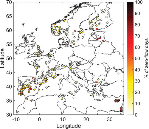
For 186 of 452 stations (41%), there are more than 10% mean annual zero-flow days (Fig. 2). As shown on the map (Fig. 2), the annual percentage of years with zero-flow days can vary strongly even for neighbouring stations. This highlights the influence of local characteristics (geology, land cover, water use, etc.) on zero-flow occurrences. The size of the river is an additional likely explanation for spatially nearby differences in intermittence, with small tributaries flowing into a larger river being more prone to drying. However, there is no clear dependency between the frequency of zero flow and catchment size, showing that other catchment characteristics that are not analysed in this study may have a stronger influence on the occurrence of zero-flow days. There is a weak latitudinal gradient in the occurrence of zero-flow days, with the higher mean annual number of zero-flow days in the south (ρ = −0.36 with latitude, significant at the 5% level), but with a very strong spatial variability even for neighbouring catchments. This implies that most intermittent streams are not necessarily associated with the most arid climate conditions in southern Europe. It must be also noted that this observation strongly depends on the density of monitoring networks and their representation of intermittent and ephemeral streams.

Figure 2. Mean annual percentage of zero-flow days for hydrological years

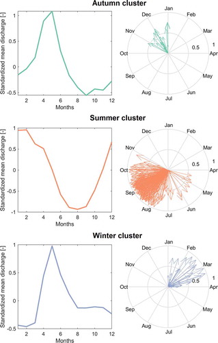
Clustering has been applied using the variables $\bar{\theta }$, the mean direction of zero flow and the variability around this date, r, computed for the winter and summer seasons. Three different seasonality patterns can be identified in Fig. 3. The largest one, the summer cluster, is composed of 376 stations having a mean date of occurrence for zero-flow days between May and November (Fig. 4). The location of the stations composing this cluster are scattered all across Europe, in different climatic zones ranging from Continental to Mediterranean climate types (Fig. 3). The second largest cluster, the winter cluster, contains 47 stations with a mean occurrence of no-flow events between January and March (Fig. 4). It includes stations with a snowmelt-driven annual regime, such as the Pyrenees or Scandinavia, that experience cessation of flow due to freezing. The autumn cluster (29 stations) corresponds to late autumn (November–January) occurrence of zero-flow days. The main difference in flow regime for the autumn and winter clusters is a more sustained runoff rate during January–March for the autumn cluster (Fig. 4), indicating that zero-flow days for the winter cluster are mostly due to freezing. As shown in this analysis, for most stations (clusters 1 and 3), the zero-flow conditions are more frequently observed in summer months, or during winter or early spring due to snow and ice cover. Yet, as shown in Fig. 3, no clear spatial patterns could be identified from this analysis although the stations belonging to the winter cluster are located predominantly in mountainous or northern areas.

Figure 3. Cluster analysis of zero-flow seasonality. Colours represent seasonality of zero-flow events classified in three clusters (winter, summer and autumn)

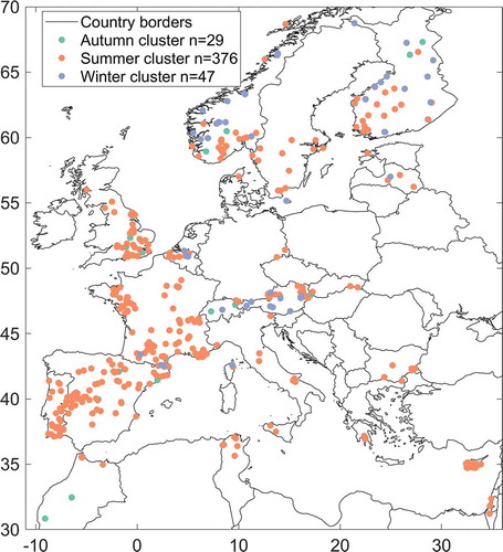
Figure 4. Flow regime (left) and mean occurrence of zero-flow days (right) for the three clusters identified in Fig. 3

4.2 Trend analysis

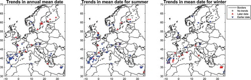
The trend detection and subsequent were performed only for the 254 rivers including at least 10 years with a minimum of 5 consecutive zero-flow days. The first trend analysis was carried out on annual, winter and summer mean dates of zero-flow occurrence, with the $\bar{\theta }$metric (Equation (4)(4) $\bar{\theta }=arcta{n}^{\ast }\left(\frac{\bar{x}}{\bar{y}}\right)$(4) ) computed on an annual or seasonal basis. The results, in terms of significant trends, indicate for most rivers located in southern Europe a trend towards earlier occurrence in zero-flow days, mostly for the annual and summer time scales (Fig. 5). For the rivers in the Baltic region, a trend towards later occurrence in zero-flow days for the summer and annual periods can be observed. Conversely, more contrasting trend patterns are detected for winter, with both positive and negative trends in the mean date for stations. A significant trend towards a later occurrence of zero flows is visible in southern France and central Spain for the winter period.

Figure 5. Significant increasing (later date) or decreasing (earlier date) trends in the mean date of zero-flow day occurrence, at the 10% significance level

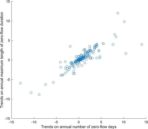
The second trend analysis concerns annual and seasonal sums and maximum lengths of zero-flow days. It should be noted that the annual number of zero-flow days and the annual maximum length of zero-flow periods are correlated, with an average correlation coefficient of 0.9 for all stations. For the summer and winter, these correlations are lower: 0.74 and 0.70, respectively.

At the annual scale, 60 stations (24%) have positive trends in the number of zero-flow days, and more generally there are more positive trends detected in comparison to negative trends for all indicators (Table 1 and Fig. 6). Overall, the trends are very similar between the extreme duration of zero-flow periods and the annual sum (Fig. 7): of the 60 stations showing a decrease in annual sum, 45 also show decreasing trends in the maximum duration of dry spells (similar behaviour is observed for positive trends). Since, on average, the trends affect about 30% of stations, these trends (both positive and negative) are field-significant according to the FDR procedure. The trend analysis results indicate that at the annual and seasonal time scales, the majority of the detected trends are towards an increase in dryness (in about 10–23% of stations, as shown in Table 1). At the seasonal time scale, there is a marked trend towards an increase in summer zero flows, but fewer trends detected for winter. When comparing trends at the annual and seasonal scales, in 60 stations with a significant increase of annual zero-flow days, 46 stations also have a significant increase in summer zero-flow days. Conversely, a lower similarity between annual and winter trends is observed. Thus, it can be concluded that the summer drying is the main driver for the decreasing trends in the number of zero-flow days at the annual scale for these stations. Overall, fewer trends are detected for extreme durations compared to annual or seasonal totals (Table 1), with the notable exception of the winter maximum lengths of zero-flow days that are increasing in the majority of stations. The results of the trend analysis were compared with catchment size, but no relationship could be found between the trends in river intermittence and the size of the basins considered.

Table 1. Summary of the detected trends in the annual and seasonal number of zero-flow days and the maximum length of dry spells

Variable	Positive trends (%)	Negative trends (%)	No trends (%)
Annual sum	23.62	10.24	66.14
Annual maximum	20.08	8.66	71.26
Winter sum	10.63	8.66	80.71
Winter maximum	23.23	9.45	67.32
Summer sum	23.62	6.69	69.69
Summer maximum	18.11%	9.45	72.44

Figure 6. Increasing (upward triangle) or decreasing (downward triangle) trends, at the 10% significance level, for the annual or seasonal mean number of zero-flow days (left), and the annual or seasonal maximum length of dry spells (right). On average, for all indicators and seasons, 28% of stations have significant trends

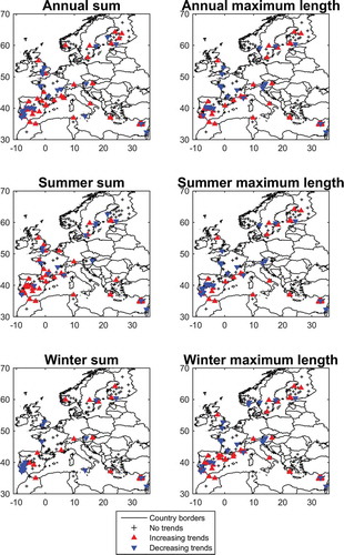
Figure 7. Scatter plot of the relationship between the Sen slope of trends in the annual number of zero-flow days and the annual maximum duration of zero-flow periods

4.3 Links with SPEI anomalies

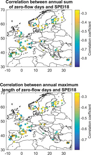
In the first step, a trend analysis was performed on SPEI over the different basins for different aggregation periods of 6, 12, 18 and 24 months. The results show a clear pattern, with positive trends at stations located north of 45°N and negative trends in the south. These trends were previously detected by Spinoni et al. (2017). At stations located north of 45ºN, due to lower temperature variability, the SPEI index responds mainly to the variability in precipitation. To check whether the SPEI anomalies could be explanatory covariates for the inter-annual variability of zero-flow day occurrences, the SPEI with different aggregation time was correlated with the number of zero-flow days and the maximum dry spell lengths. The results show a strong association of zero-flow days with SPEI anomalies in particular at the annual and summer time scales, with significant correlations in more than half of the stations (Fig. 8), with a lower number of significant correlations during winter. The annual or seasonal sums of zero-flow days are more strongly associated with SPEI anomalies than are the maximum lengths of dry spells. The correlations are negative for all SPEI time scales (Fig. 9), indicating that negative SPEI anomalies, i.e. pronounced net precipitation deficits, are linked with a larger number of zero-flow days.

Figure 8. Significant correlations at the 5% level between annual, summer and winter sum of zero-flow days, and the maximum length of dry periods with SPEI over the different basins for different aggregation periods of 6, 12, 18 and 24 months (Standardized Precipitation Evapotranspiration Index) (SPEI6, SPEI12, SPEI18 and SPEI24, respectively)

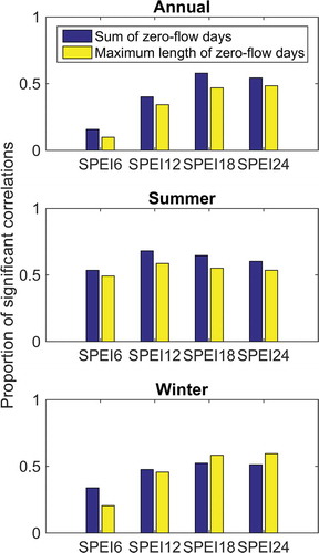
Figure 9. Map of the significant correlations between the annual sum of zero-flow days (top) and the annual maximum length of zero-flow days (bottom) with the (Standardized Precipitation Evapotranspiration Index) SPEI18. Crosses indicate stations where the correlation is not significant at the 10% level. Correlations are negative because the smaller the SPEI (water deficit), the larger the number of zero-flow days

For about one-third of stations (36%), there are no significant correlations. These stations are mostly located in Spain, southern France, North Africa and Cyprus, but also Belgium, without a clear spatial pattern. Therefore, a strong variability of the spatial pattern is once again evident, indicating local influences on the relationship between zero-flow days and SPEI. The strength of the correlations is higher for basins with a larger annual average number of zero-flow days for almost all SPEI time scales. This demonstrates that strongly intermittent basins (i.e. basins with a large proportion of zero-flow days) are more influenced by climatic variations to determine the annual number of zero-flow days. This is probably due to the fact that these streams are often close to the wet/dry threshold and consequently immediately impacted by a variation of precipitation availability. There is also a statistically significant but moderate (ρ = 0.2) correlation between the strength of the correlations with the SPEI12 and basin size. This indicates that the influence of SPEI12 might be stronger for smaller basins since larger basins are more likely to be more influenced by human activities, while small basins respond more quickly to precipitation and might have lower local water storage capacity. Yet this relationship is not significant for the SPEI18 and SPEI24. Smaller basins have a reduced water storage capability in the context of climate variability, so this behaviour is expected.

4.4 Relations with large-scale atmospheric circulation

As the large-scale climate drivers have a low-frequency time variability, the correlation analysis should consider long time series. This is the reason why only rivers with at least 30 years of data during 1970–2010 have been considered to analyse the relationships with large-scale circulation indices. The AMO and NAO are the most influential climate indices on zero-flow occurrences. Since very low correlations were found with the other indices, we focus the analysis on the results with AMO and NAO. At the annual scale, the AMO was the index with the highest number of positive correlations: 21% for the longest annual no-flow event and 23% for the annual sum. Results for both metrics in different seasons are presented in Table 2. The summer and the winter AMO are the drivers with the strongest links to the summer and winter metrics. A cluster of rivers positively associated with the winter AMO is easily recognizable in northern Europe (Norway, Finland) for both winter metrics (FFig. 10). Northern regions, including the UK and south Sweden, exhibit a negative link between winter AMO and the winter sum of zero-flow days. A similar pattern is observed for the summer with annual AMO. Additionally, the southern Mediterranean part of Europe might be positively influenced by the summer AMO.

Table 2. Summary of catchments with significant correlations ($\alpha =0.05$) between seasonal metrics of intermittence and large-scale climate drivers. Subscripts $s,w,$ DJF, JJA, w1 refer to the summer (April–September), winter (September–March), December–February, June–August, and winter from the preceding year, respectively

(a)	Positive correlation		Negative correlation	(b)	Positive correlation
Variable	AMOs	AMOw	NAODJF	Variable	NAOJJA	AMOs	AMOw1
Winter max	18%	16%	11%	Summer max	11%	21%	18%
Winter sum	21%	19%	11%	Summer sum	9%	22%	21%

Figure 10. Significant correlations between summer zero-flow days and Atlantic Multi-decadal Oscillation (AMO) (left) and between winter zero-flow days and North Atlantic Oscillation (NAO) (right)

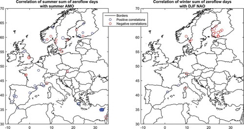
It can be concluded that the AMO is a potential driver of the intermittence in about 20% of stations and its influence can be stretched to the following season. The associations with the NAO are less frequent. However, the apparent cluster of rivers with a negative link to the winter NAO can be observed in the Scandinavian Peninsula for both winter metrics (Fig. 10). The rivers positively linked to JJA NAO are scattered over Europe. It is worth emphasizing that this large-scale climate effect can be obscured by more local climate conditions. The relationship between climate drivers and hydrological characteristics in Europe has been previously documented by many researchers (e.g. Wrzesiński and Paluszkiewicz 2011, Valty et al. 2015). Results of the present analysis are to a large extent consistent with those obtained by Hurrell and Folland (2002), Linderholm et al. (2009), Giuntoli et al. (2013), indicating that the NAO and AMO could influence hydrological droughts.

5 Discussion and conclusions

This study provides the first European-scale assessment of the trends in river intermittence over the last few decades. The most striking results are (a) the strong spatial variability of the detected trends, and (b) the seasonality and relationships with climate drivers. Overall, there is considerable spatial variability of flow intermittence. Snelder et al. (2013) previously observed over France that the high spatial heterogeneity in small-scale processes associated with intermittence partly explains the low spatial synchronization of zero flows. Significant trends are detected in about 30% of stations, with most of the detected trends towards an increasing number of zero-flow days, tending to occur earlier in the season, in particular around the Mediterranean basin. For most basins, there is a strong association of zero-flow days with SPEI negative anomalies, but neighbouring basins may exhibit different relationships, again showing the strong spatial variability. This indicates that the SPEI could be a valid predictor for zero-flow occurrence, and the decreasing trend in this indicator observed over southern Europe may explain the trends in flow intermittence obtained in this study. Recent studies have shown that these downward trends in SPEI are mostly explained by an increase in the atmospheric evaporative demand rather than a decline in precipitation (Vicente-Serrano et al. 2020, Peña-Angulo et al. 2020). In a climate change context with increasing temperatures, it is likely that this trend will continue in the future, with a possible increase in river intermittence for these regions.

The strong spatial variability observed in trends in intermittence characteristics implies that regional predictions or generalizations for flow intermittence patterns should be interpreted with caution. Any mapping or extrapolation from such regional results may be prone to considerable errors if not considering basin characteristics that are likely to play a strong role in determining flow intermittence properties. In this study, the individual catchment characteristics (i.e. topography, geology, land use, soil types) have not been analysed, which would require major work at such a continental-wide scale. Catchment characteristics may be helpful to distinguish the different patterns in flow intermittence since, as shown in this study, the geographical location and basin size do not exert a strong control on river intermittence. In particular, it would be interesting to distinguish basins with strong surface–groundwater interactions that could explain some of the patterns described in the present study. However, as noted by Snelder et al. (2013), flow intermittence is also controlled by processes operating at scales smaller than catchments, thus capturing these processes would require a much more detailed investigation than classical regional approaches to take into account the local physiographic characteristics (Tramblay et al. 2010).

A major uncertainty of the work presented herein – and, to a greater extent, applicable to all ecohydrological research on intermittent rivers – is the definition of the zero-flow days and the lack of regional representativeness of the monitoring networks. With regard to the first aspect, there is a wide variety of measurement procedures in different European countries, leading to differing accuracy of the measured discharge values, in particular the minimal values. For example, in the UK or in France the data is provided in m³ s⁻¹, with an accuracy of three decimal places, but for many other countries, the minimum reported discharge is sometimes much greater than 1 L s⁻¹, due to different measuring methods. In addition, many rating curves at open-channel stations have uncertainty at low flows caused by instability of the riverbed. In the present work, we considered a strict criterion to identify zero-flow days, but a more adequate selection could be made possible if good-quality metadata information were available for most rivers, which is not currently the case for several countries. With regard to the second aspect, of regional representativeness, several studies have highlighted the lack of measurements for intermittent rivers (Skoulikidis et al. 2017, Costigan et al. 2017). The number of monitored headwater streams which are likely to be intermittent is indeed much smaller than the number of perennial and large streams in national and international databases, although their contribution to the water resources is probably high. This calls into question the rationale behind national measurement strategies for intermittent streams, in particular the most ephemeral ones, since they may be overlooked in water resource management in comparison to perennial streams. Depending on the national monitoring strategies of the river network, it is possible that the selection of intermittent rivers to be monitored may be biased towards a specific type of rivers within a given geographic location of geological properties.

Another important aspect to take into consideration is the regulation status of the monitored rivers, which may evolve over time and not be available in the stations’ metadata. In this work, the selected basins are those described as natural or weakly altered based on their metadata information. Yet how does one quantitatively define “weakly altered” between different national networks and monitoring protocols? This definition may differ from one country to another without a common objective criterion to define the percentage of natural discharge being diverted or used for water supply. Besides river alterations, often assumed to be a matter of expert judgement, quantitative evaluation of the water uptake would require extensive work to monitor and collect water consumption data over time. Even for a river considered to be unaltered, diffuse groundwater pumping may occur and may therefore have impacts on the groundwater–surface water interactions, which could in turn strongly impact intermittence occurrence. Two examples of the influence of river status, as described in the metadata, on the trend results may be found in the UK. The Coal Burn River is classified as broadly natural but is in fact an experimental catchment set up to assess the impact of afforestation, and the trend analysis indicates an increase in zero-flow days, showing that the influence of land-use change might indeed be significant on this aspect of the flow regime. The limestone Slea River that, conversely, experienced a decrease in zero-flow days was also classified as natural, but further scrutiny revealed a discharge augmentation scheme installed in 1995. Taking into account all these local specificities in addition to the available metadata would require tremendous effort, and such information may not always be as readily available. The main findings of the present study are an incentive to implement process-based studies on the intermittence characteristics for different climatic and physiographic environments, taking into account watershed characteristics.

Acknowledgements

This research is part of the COST action CA15113 SMIRES, Science and Management of Intermittent Rivers and Ephemeral Streams https://www.smires.eu/, a short-term scientific mission that has been funded for Agnieszka Rutkowska. Agnieszka Rutkowska was also supported by the Ministry of Science and Higher Education of the Republic of Poland (grant DS 3371). The different data providers are gratefully acknowledged. Some of the station data were retrieved from the Global Runoff Data Centre (56068 Koblenz, Germany) and from the HyMeX programme database. The authors would like to thank two anonymous reviewers, Kendra Kaiser and the Associate Editor, Stephanie Kampf, for their constructive comments.

Disclosure statement

No potential conflict of interest was reported by the authors.

Data availability statement

The indices computed in the present work will be made available to the community for research applications upon request to the first author.

Correction Statement

This article has been republished with minor changes. These changes do not impact the academic content of the article.

References

- Beaufort, A., Carreau, J., and Sauquet, E., 2019. A classification approach to reconstruct local daily drying dynamics at headwater streams. Hydrological Processes, 33 (13), 1896–1912. doi:10.1002/hyp.13445.
- Beguería, S., et al., 2014. Standardized precipitation evapotranspiration index SPEI revisited: parameter fitting, evapotranspiration models, tools, datasets and drought monitoring. International Journal of Climatology, 34 (10), 3001–3023. doi:10.1002/joc.3887.
- Benjamini, Y. and Hochberg, Y., 1995. Controlling the false discovery rate: A practical and powerful approach to multiple testing. Journal of the Royal Statistical Society, Series B, 57, 289–300.
- Bormann, H. and Pinter, N., 2017. Trends in low flows of German rivers since 1950: comparability of different low‐flow indicators and their spatial patterns. River Research and Applications, 33 (7), 1191–1204. doi:10.1002/rra.3152.
- Burn, D.H., 1997. Catchment similarity for regional flood frequency analysis using seasonality measures. Journal of Hydrology, 202 (1–4), 212–230. doi:10.1016/S0022-1694(97)00068-1.
- Coch, A. and Mediero, L., 2016. Trends in low flows in Spain in the period 1949–2009. Hydrological Sciences Journal, 61 (3), 568–584. doi:10.1080/02626667.2015.1081202.
- Costigan, K., et al., 2017. Chapter 2.2 – flow regimes in intermittent rivers and ephemeral streams. In: T. Datry, N. Bonada, and A.J. Boulton, eds.. Intermittent rivers and ephemeral streams. Ecology and management. Amsterdam: Academic Press, 51–78. doi:10.1016/c2015-0-00459-2.
- D’Ambrosio, E., et al., 2017. Characterising the hydrological regime of an ungauged temporary river system: a case study. Environmental Science and Pollution Research, 24 (16), 13950–13966. doi:10.1007/s11356-016-7169-0.
- Datry, T., et al., 2017. Science and management of intermittent rivers and ephemeral streams SMIRES. Research Ideas and Outcomes, 3, e21774. doi:10.3897/rio.3.e21774
- De Girolamo, A.M., et al., 2017. Hydrology under climate change in a temporary river system: potential impact on water balance and flow regime. River Research and Applications, 33 (7), 1219–1232. doi:10.1002/rra.3165.
- Delso, J., Magdaleno, F., and Fernández-Yuste, J.A., 2017. Flow patterns in temporary rivers: a methodological approach applied to southern Iberia. Hydrological Sciences Journal, 62 (10), 1551–1563. doi:10.1080/02626667.2017.1346375.
- Döll, P. and Schmied, H.M., 2012. How is the impact of climate change on river flow regimes related to the impact on mean annual runoff? A global-scale analysis. Environmental Research Letters, 7 (1), 14037. doi:10.1088/1748-9326/7/1/014037.
- Dörflinger, G., 2016. A new spatial basis for rivers monitoring and management in Cyprus. DProf thesis. Middlesex University. [online]. Available from: http://eprints.mdx.ac.uk/20817/ [ accessed 15 January 2020].
- Eng, K., Wolock, D.M., and Dettinger, M.D., 2016. Sensitivity of intermittent streams to climate variations in the USA. River Research and Applications, 32 (5), 885–895. doi:10.1002/rra.2939.
- Gallart, F., et al., 2010. Investigating hydrological regimes and processes in a set of catchments with temporary waters in Mediterranean Europe. Hydrological Sciences Journal, 53 (3), 618–628. doi:10.1623/hysj.53.3.618.
- Gallart, F. and Llorens, P., 2004. Observations on land cover changes and water resources in the headwaters of the Ebro catchment, Iberian Peninsula. Physics and Chemistry of the Earth, Parts A/B/C, 29 (11–12), 769–773. doi:10.1016/j.pce.2004.05.004.
- Giuntoli, I., et al., 2013. Low flows in France and their relationship to large scale climate indices. Journal of Hydrology, 482, 105–118. doi:10.1016/j.jhydrol.2012.12.038
- Gustard, A., Bullock, A., and Dixon, J.M., 1992. Low flow estimation in the United Kingdom. Report No. 108, Institute of Hydrology, Wallingford, UK. 292p.
- Hamed, K.H. and Rao, A.R., 1998. A modified Mann-Kendall trend test for autocorrelated data. Journal of Hydrology, 204 (1–4), 182–196. doi:10.1016/S0022-1694(97)00125-X.
- Hannaford, J., et al., 2011. Examining the large-scale spatial coherence of European drought using regional indicators of precipitation and streamflow deficit. Hydrological Processes, 25 (7), 1146–1162. doi:10.1002/hyp.7725.
- Hertig, E. and Tramblay, Y., 2017. Regional downscaling of Mediterranean droughts under past and future climatic conditions. Global and Planetary Change, 151, 36–48. doi:10.1016/j.gloplacha.2016.10.015
- Hurrell, J.W. and Folland, C.K., 2002. The relationship between tropical Atlantic rainfall and the summer circulation over the North Atlantic. CLIVAR Exchanges, 25, 52–54.
- Ionita, M., et al., 2017. The European 2015 drought from a climatological perspective. Hydrology and Earth System Sciences, 21, 1397–1419. doi:10.5194/hess-21-1397-2017
- Kennard, M.J., et al., 2010. Classification of natural flow regimes in Australia to support environmental flow management. Freshwater Biology, 55 (1), 171–193. doi:10.1111/j.1365-2427.2009.02307.x.
- Kirkby, M.J., et al., 2011. Classifying low flow hydrological regimes at a regional scale. Hydrology and Earth System Sciences, 15 (12), 3741–3750. doi:10.5194/hess-15-3741-2011.
- Laaha, G. and Blöschl, G., 2006. Seasonality indices for regionalizing low flows. Hydrological Processes, 20 (18), 3851–3878. doi:10.1002/hyp.6161.
- Laaha, G., et al., 2017. The European 2015 drought from a hydrological perspective. Hydrology and Earth System Sciences, 21 (6), 3001–3024. doi:10.5194/hess-21-3001-2017.
- Linderholm, H.W., Folland, C.K., and Walther, A., 2009. A multicentury perspective on the summer North Atlantic Oscillation SNAO and drought in the eastern Atlantic Region. Journal of Quaternary Science, 24 (5), 415–425. doi:10.1002/jqs.1261.
- Mann, H.B., 1945. Nonparametric tests against trend. Econometrica, 13 (3), 245–259. doi:10.2307/1907187.
- Marx, A., et al., 2018. Climate change alters low flows in Europe under global warming of 1.5, 2, and 3 °C. Hydrology and Earth System Sciences, 22 (2), 1017–1032. doi:10.5194/hess-22-1017-2018.
- McKee, T.B., Doesken, N.J., and Kleist, J., 1993. The relationship of drought frequency and duration to time scales. Proceedings of the 8th Conference on Applied Climatology, American Meteorological Society, 179–184, Anaheim, CA.
- Myronidis, D., et al., 2018. Streamflow and hydrological drought trend analysis and forecasting in Cyprus. Water Resources Management, 32 (5), 1–18. doi:10.1007/s11269-018-1902-z.
- Osuch, M., Romanowicz, R.J., and Wong, W.K., 2018. Analysis of low flow indices under varying climatic conditions in Poland. Hydrology Research, 49 (2), 373–389. doi:10.2166/nh.2017.021.
- Oueslati, O., et al., 2015. Classifying the flow regimes of Mediterranean streams using multivariate analysis. Hydrological Processes, 29 (22), 4666–4682. doi:10.1002/hyp.10530.
- Peña-Angulo, D., et al., 2020. Precipitation in Southwest Europe does not show clear trend attributable to anthropogenic forcing. Environmental Research Letters, 15 (9), 094070. doi:10.1088/1748-9326/ab9c4f.
- Perez-Saez, J., et al., 2017. Classification and prediction of river network ephemerality and its relevance for waterborne disease epidemiology. Advances in Water Resources, 110, 263–278. doi:10.1016/j.advwatres.2017.10.003
- Pournasiri Poshtiri, M., et al., 2019. Variability patterns of the annual frequency and timing of low streamflow days across the United States and their linkage to regional and large‐scale climate. Hydrological Processes, 33 (11), 1569–1578. doi:10.1002/hyp.13422.
- Skoulikidis, N.T., et al., 2017. Non-perennial Mediterranean rivers in Europe: status, pressures, and challenges for research and management. Science of the Total Environment, 577, 1–18. doi:10.1016/j.scitotenv.2016.10.147
- Snelder, T.H., et al., 2013. Regionalization of patterns of flow intermittence from gauging station records. Hydrology and Earth System Sciences, 17 (7), 2685–2699. doi:10.5194/hess-17-2685-2013.
- Spinoni, J., Naumann, G., and Vogt, J.J., 2017. Pan-European seasonal trends and recent changes of drought frequency and severity. Global and Planetary Changes, 148, 113–130. doi:10.1016/j.gloplacha.2016.11.013
- Stahl, K. and Demuth, S., 1999. Linking streamflow drought to the occurrence of atmospheric circulation patterns. Hydrological Sciences Journal, 44 (3), 467–482. doi:10.1080/02626669909492240.
- Stahl, K., et al., 2010. Streamflow trends in Europe: evidence from a dataset of near-natural catchments. Hydrology and Earth System Sciences, 14 (12), 2367–2382. doi:10.5194/hess-14-2367-2010.
- Tramblay, Y., et al., 2010. Estimation of local extreme suspended sediment concentrations in California Rivers. Science of the Total Environment, 408 (19), 4221–4229. doi:10.1016/j.scitotenv.2010.05.001.
- Tzoraki, O., et al., 2016. Assessing the Flow alteration of temporary streams under current conditions and changing climate by SWAT model. International Journal of River Basin Management, 14 (1), 1571–5124. doi:10.1080/15715124.2015.1049182.
- Valty, P., et al., 2015. Impact of the North Atlantic Oscillation on Southern Europe Water Distribution: insights from Geodetic Data. Earth Interactions, 19 (10), 1–16. doi:10.1175/EI-D-14-0028.1.
- Vicente-Serrano, S.M., Beguería, S., and Lopez-Moreno, J.I., 2010. A multiscalar drought index sensitive to global warming: the standardized precipitation evapotranspiration index – SPEI. Journal of Climate, 23 (7), 1696–1718. doi:10.1175/2009JCLI2909.1.
- Vicente-Serrano, S.M., et al., 2020. Long-term variability and trends in meteorological droughts in Europe (1851–2018). International Journal of Climatology. doi:10.1002/joc.6719.
- Ward, J.H., 1963. Hierarchical grouping to optimize an objective function. Journal of the American Statistical Association, 58 (301), 236–244. doi:10.1080/01621459.1963.10500845.
- Wilks, D.S., 2016. The stippling shows statistically significant grid points: how research results are routinely overstated and overinterpreted, and what to do about it. Bulletin of the American Meteorological Society, 97 (12), 2263–2273. doi:10.1175/BAMS-D-15-00267.1.
- Wrzesiński, D. and Paluszkiewicz, R., 2011. Spatial differences in the impact of the North Atlantic Oscillation on the flow of rivers in Europe. Hydrology Research, 42 (1), 30–39. doi:10.2166/nh.2010.077.
- Zimmer, M.A., et al., 2020. Zero or not? Causes and consequences of zero‐flow stream gage readings. WIREs Water, Wiley. 7. doi:10.1002/wat2.1436.