When does a parsimonious model fail to simulate floods? Learning from the seasonality of model bias

ABSTRACT

Identifying situations where a hydrological model yields poor performance is useful for improving its predictive capability. Here we applied an evaluation methodology to diagnose the weaknesses of a parsimonious rainfall-runoff model for flood simulation. The GR5H-I hourly lumped model was evaluated over a large set of 229 French catchments and 2990 flood events. Model bias was calculated considering different streamflow time windows, from calculations using all observations to analyses of individual flood events. We then analysed bias across seasons and against several flood characteristics. Our results show that although GR5H-I had good overall performance, most of the summer floods were underestimated. In summer and autumn, compensations between flood and recession periods were identified. The largest underestimations of flood volumes were identified when high-intensity precipitation events occurred, especially under low soil moisture conditions.

KEYWORDS:

• hydrological modelling
• flood simulation
• model bias
• model diagnostic
• seasonality

Editor A. Castellarin Associate editor A. Petroselli

1 Introduction

1.1 On the need to improve hydrological models for flood forecasting

Reliable hydrometeorological predictions are important for mitigating the hazards associated with floods, including loss of lives and livelihoods as well as economic losses (e.g. Carsell et al. 2004, Hallegatte 2012, Jeuland et al. 2019). Many operational flood forecasting systems have been implemented around the world to produce streamflow forecasts (Pappenberger et al. 2016) and hydrological models are the basis of these flood forecasting systems (Pagano et al. 2014). However, streamflow predictions produced by these models are still subject to large uncertainties (Roundy et al. 2018). Different sources of uncertainty can affect the predictive capability of hydrological models (e.g. Beven 2016). These uncertainties can be related to the input data, model parameterization or model structural deficiencies, for example. Consequently, advances in hydrological modelling are needed to obtain more accurate estimates of flood peak, timing and volume, and therefore issue earlier and better warnings (e.g. Pagano et al. 2014, Jain et al. 2018). Flood forecasting systems have been improved over the years (e.g. Zanchetta and Coulibaly 2020). For example, the use of continuous models instead of event-based models allowed a reduction of the uncertainty associated with initial conditions (e.g. Berthet et al. 2009, Grimaldi et al. 2020). However, common failures to predict floods are still encountered. For example, the severe floods that occurred in the Seine and Loire rivers and their tributaries (France) in June 2016 were underestimated by our own GRP flood forecasting model (Berthet 2010, Viatgé et al. 2019). Hydrological models are also less reliable in arid or dry areas (e.g. McMillan et al. 2016, Melsen et al. 2018), especially when flash floods occur (Hapuarachchi et al. 2011). Improving the predictive capability of hydrological models is therefore essential for improved flood forecasting.

1.2 Relevance of large-sample model diagnostics

To be able to improve a model, one must first identify situations where the model fails to yield reliable results, i.e. the first-order factors leading to simulation errors (Gupta et al. 2008). In this regard, various diagnostic methods have been used on hydrological models. Some studies were based on a limited number of catchments (e.g. Butts et al. 2004, Clark et al. 2008, Nicolle et al. 2014). Diagnostics are now increasingly relying on large-sample approaches in order to draw more general conclusions from model performance (e.g. Andréassian et al. 2009, Gupta et al. 2014). Large-sample studies make it possible to establish performance benchmarks, i.e. to determine the current performance of hydrological models across a representative set of catchments (e.g. Seibert 2001, Seibert et al. 2018). The effects of changes in, for instance, model structure or parameterization can then be assessed in light of the performance of the benchmark. Several recently published country-scale studies investigate different model structures over large sets of catchments representing a variety of hydroclimatic conditions. For example, Lane et al. (2019) investigated the predictive capability of four models over 1000 catchments in the UK and the relationships between model performance and catchment attributes, flow regimes and model structures. Knoben et al. (2020) compared the performance of 38 models over 559 US catchments and highlighted groups of models for which the structural hypotheses were better suited for some catchments rather than others (e.g. seven models had better performance for flashy catchments).

1.3 Model evaluation issues

One of the challenges of large-sample hydrology is related to the advantage of exploiting the robust statistical properties of large samples (Mathevet et al. 2006, 2020) while summarizing the results into an understandable outcome but still maintaining a certain degree of precision to find emerging patterns (Gupta et al. 2014). Many large-sample studies used aggregated statistics to assess model performance across comprehensive datasets (e.g. Perrin et al. 2008, Vaze et al. 2010, 2011, Coron et al. 2012, Andréassian et al. 2014). Some comparative studies of rainfall-runoff models found similar levels of performance between model structures when using aggregated metrics (e.g. Perrin et al. 2001, Van Esse et al. 2013). It has been widely recognized that the use of single aggregated metrics is not sufficient to assess model performance (e.g. Schaefli and Gupta 2007, Euser et al. 2013). For example, Mathevet et al. (2020) compared the performance of two conceptual models across a global set of catchments within a multi-objective framework. They found that while the two models yielded similar overall performance, when looking at sub-period statistics, one model performed slightly better in short-term processes. Furthermore, commonly used performance indicators, such as the Nash-Sutcliffe efficiency criterion (NSE; Nash and Sutcliffe 1970), are known to be biased towards high flows, although their use in model calibration leads to underestimation of flow variability (Gupta et al. 2009) and a limited ability to reproduce extreme flows (Oudin et al. 2006, Crochemore et al. 2015). Therefore they must be used cautiously when evaluating the ability of models to simulate floods.

Hydrological signatures have been found useful in improving the identification of patterns between model performance and our understanding of underlying catchment processes (Yilmaz et al. 2008, Hrachowitz et al. 2014, McMillan et al. 2017). They are used as indicators of situations where models perform well and are suitable for further applications. Consequently, a growing number of studies are using sets of hydrological signatures for model evaluation to emphasize particular aspects of the hydrograph (e.g. Shafii and Tolson 2015, Donnelly et al. 2016, Poncelet et al. 2017, Gnann et al. 2020). Signatures to investigate model performance on high flows can be, for example, the runoff volume above the 80^th percentile of the flow duration curve (Yilmaz et al. 2008). Another way to highlight model errors in flood predictions is to evaluate the simulation of peak flows by calculating specific criteria, such as the time to peak or the peak flow ratio. For example, Mizukami et al. (2019) investigated the choice of objective functions to better simulate high flows by calculating the annual peak flow bias.

1.4 A focus on events and seasonality

Event-based models are usually evaluated by their ability to reproduce several flood characteristics, such as rising limb, peak flow magnitude or timing (e.g. Borah et al. 2007, Javelle et al. 2010, Stanić et al. 2018, Stephens et al. 2018). To focus on the ability of continuous models to reproduce floods, model performance can also be assessed against a set of events in streamflow time series. By selecting 3620 flood events in 181 catchments, Lobligeois et al. (2014) identified where and when accounting explicitly for the spatial variability of rainfall and potential evapotranspiration inputs (i.e. by using a semi-distributed approach) improved streamflow simulations. Ficchì et al. (2016) showed that the peaks and timing of 2400 floods in 240 catchments were better reproduced at sub-daily time steps than at a daily time step. Vergara et al. (2016) evaluated the regionalization of the parameters of a hydraulic routing function by calculating peak flow and timing errors in the simulation of 47 563 flood events. de Boer-Euser et al. (2017) compared eight hydrological models in one catchment and found similar results in terms of overall performance but clear differences when looking at specific events and metrics. For different purposes, these studies showed that a change of focus in model evaluation, e.g. investigating flood events, can help to identify patterns in the performance of hydrological models.

Streamflow can have strong seasonal variations depending on climate seasonality and catchment characteristics (Berghuijs et al. 2014, Gnann et al. 2020). The seasonal streamflow variations also reflect varying antecedent soil moisture conditions, which can have significant impacts on flood event generation (Blöschl et al. 2013, Berghuijs et al. 2014). In terms of model diagnostics, some studies used signatures to assess the ability of the models to simulate the streamflow regime (e.g. Wang et al. 2008, Massmann 2020). Other model evaluations investigating the seasonality of model performance relied on the analysis of metrics calculated for each season of the year independently (e.g. Muleta 2012, Kim and Lee 2014, Lane et al. 2019).

1.5 Scope of the paper

While it is clear that analysing the performance of hydrological models in simulating flood events can help to characterize model performance, a deeper investigation on the seasonality of model performance considering different streamflow time windows has, to our knowledge, not been conducted to date. In an effort to find patterns of model errors and therefore help target model improvements, we apply a new methodology to assess the simulations of a continuous conceptual rainfall-runoff model over a large sample of flood events at an hourly time step. Bennett et al. (2013) suggested that, to evaluate environmental models, we must first look at basic performance criteria and then refine the analyses depending on the problem at hand. Here we follow these recommendations and aim to probe deeper in the analyses by looking at the seasonality of model bias through different disaggregations of the observed hydrograph. The objectives of this paper are (i) to determine whether investigating the seasonality of model bias through different streamflow time windows can provide information on model deficiencies in simulating high flows and (ii) to identify factors causing model weaknesses in flood simulations.

2 Data

2.1 Catchment set

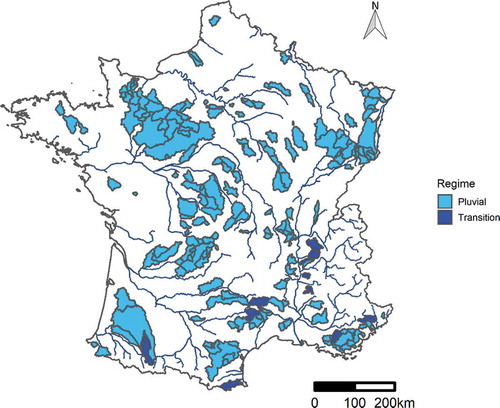
A total of 229 catchments in France were selected, representing varying hydroclimatic and morphological characteristics (Fig. 1). This catchment selection originates from the work of Ficchì et al. (2016). Snow and human activities have limited impacts on the streamflow of these catchments. Eleven catchments were discarded from the original set because of low-quality data, a too-high percentage of missing streamflows or a high solid precipitation fraction (i.e. with more than 10% of solid precipitation). A summary of the catchment set characteristics is given in Table 1. Further information can be found in the studies by Ficchì et al. (2016) and Ficchì (2017). The baseflow index values higher than 0.9 correspond to two catchments located in the northern part of France, where flow is dominated by the contribution of a dual-porosity chalk aquifer. Two karstic catchments, the Laine River at Soulaines-Dhuy and the Siagne River at Callian, are included in our dataset and have runoff coefficients higher than 1. Flashy catchments, i.e. with high-intensity precipitation and low values of flow autocorrelation, are mainly located in the Mediterranean region and in the Cévennes area in southern France. A large part of the catchments in our dataset are characterized by pluvial streamflow regimes (as defined by Sauquet et al. 2008), where most periods of high flows are in winter and most periods of low flows are in summer. Fourteen catchments are in the transition regime, meaning that high flows occur in winter and spring because of the influence of both rainfall and snowmelt. We chose to keep these catchments for our analyses because Valéry (2010) showed that the sensitivity of model simulations to snow dynamics is limited when the part of solid precipitation is less than 10%.

Table 1. Distribution of nine hydroclimatic and five morphological characteristics of 229 catchments. P99 is the 99^th percentile of daily streamflow

Characteristic	Definition/reference	Min	Q25	Med	Mean	Q75	Max
Area [km^2]	-	3.54	164.1	354.1	680.3	772.3	7918
Average altitude [m]	-	70	198	358	383	519	1060
Average slope [-]	-	0.01	0.03	0.05	0.06	0.08	0.24
Topographic index [-]	Ducharne (2009)	8.19	12.13	13.26	13.13	14.25	17.33
Drainage density [km^2]	Le Moine (2008)	0.06	0.3	0.51	1.19	1.08	19.8
Mean flow (Qm) [mm/year]	-	35	262	349	437	524	1398
Mean annual temperature (°C)	-	8.2	9.8	10.4	10.6	11.1	14.3
Fraction of solid precipitation (%)	-	0.5	2.2	3.1	4.1	5.9	9.4
Mean annual precipitation	-	651	818	937	990	1097	2108
(Pm) [mm] Mean annual potential	-	594	664	708	739	767	1129
Evapotranspiration (PEm) [mm/year] Flow auto-correlation at 24 h [-]	-	0.39	0.77	0.84	0.83	0.91	1.00
Runoff coefficient [-]	Qm/Pm	0.04	0.27	0.35	0.38	0.46	1.71
Aridity index [-]	Pm/PEm	0.66	1.10	1.32	1.37	1.55	3.47
Daily precipitation intensity [-]	P99/Pm	7.58	8.57	9.19	10.56	11.53	19.89
Baseflow index [-]	Gustard et al. (1992)	0.19	0.46	0.57	0.56	0.65	0.95
Rainfall-runoff lag time [h]	Ficchì (2017)	1	8	15	21	26	117

Figure 1. Location of the 229 French catchments selected. The streamflow regimes were determined according to the definition of Sauquet et al. (2008)

2.2 Hydroclimatic data

Time series of precipitation at an hourly time step were aggregated at the catchment scale from the Comephore product (Tabary et al. 2012), provided by Météo-France at a 1-km resolution over the French metropolitan territory. Comephore offers a quantitative precipitation reanalysis combining all of the available information from weather radars and rain gauges. The time series of daily temperature extracted by Delaigue et al. (2020) from the SAFRAN climate reanalysis database of Météo-France (Vidal et al. 2010) were used to calculate potential evapotranspiration (PE) time series with the Oudin et al. (2005) formula. The daily PE time series were then disaggregated at the hourly time step by assuming a parabolic shape from 6:00 a.m. to 7:00 p.m. (UTC). The maximum PE values are between 12:00 a.m. and 1:00 p.m. Instantaneous streamflow data from the database of the French hydrometric services (Leleu et al. 2014) were interpolated to obtain hourly time series. Precipitation, temperature and streamflow time series covered the period from 1 August 2005 to 31 July 2013. Two independent sub-periods were considered: P1, from 1 July 2005 to 31 June 2009; and P2, from 1 July 2009 to 31 June 2013. For most catchments, these periods are similar in terms of mean runoff coefficient and PE. Differences in the runoff coefficient higher than 5% between P1 and P2 are found in only three tributaries of the Rhône River (downstream): the Ardèche River at Ucel, the Cèze River at Tharaux and at Montclus, and the Argens River at Arcs located in the Mediterranean area.

2.3 Selection of flood events

An automated procedure was used to select 2990 flood events in the catchment dataset: 1681 events in P1 and 1309 events in P2. On average, 13 events were selected per catchment. The number of selected events ranges from 3 to 16 events per catchment. Only events with peak flow higher than the 95^th streamflow quantile were selected. Flood event periods were taken from the time when streamflow is higher than 20% of the event peak flow to the time when streamflow is lower than 30% of the event peak flow. Each flood event was then visually inspected to avoid overlaps and other errors arising from the automated selection procedure. Figure 2 illustrates some of the flood event characteristics per season. In Fig. 2(c), the ratio of flood volume to total water volume was computed as the ratio between the volume of each flood and the total water volume.

Figure 2. Distribution and localization of the characteristics of 2990 flood events. The distributions are presented between the 5^th and 95^th percentiles. Parts (b) and (d) present maximum values and part (f) presents mean values. n_ev is the number of flood events of each season and n_c is the related number of catchments

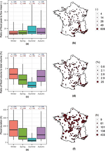
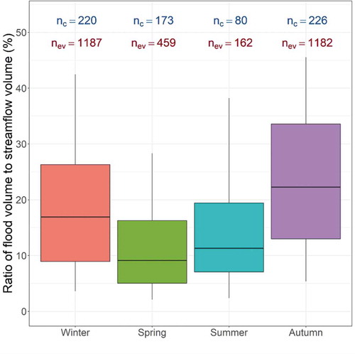
Winter was considered to extend from the beginning of January to the end of March, spring from April to June, summer from July to September, and autumn from October to December. The highest flow peaks relative to mean catchment flow occurred in summer and autumn, mostly in tributaries of the Rhône River and in the Mediterranean region. Summer events are shorter and lower in volume than the other flood events in our dataset. Figure 3 shows that the volume of the selected events ranges from 2% (spring 5^th percentile) to 45% (autumn 95^th percentile) of the total streamflow volume of the corresponding season. The spring events represent a smaller fraction of the overall spring streamflow volume, whereas autumn events represent a larger proportion of the streamflow volume of the corresponding season.

Figure 3. Distribution of catchment seasonal flood volumes compared with seasonal streamflow volume for 2990 flood events in 229 catchments. n_ev is the number of flood events of each season and n_c is the related number of catchments

3 Methods

3.1 Hydrological model and parameter calibration

The continuous GR5H lumped conceptual rainfall-runoff model (Le Moine 2008, Lobligeois 2014) was used to simulate streamflow hourly time series at the outlet of each catchment. We used a version that integrates an interception store (GR5H-I), as formulated by Ficchì et al. (2019). Full mathematical details of the model are given in the Appendix. We performed a continuous split-sample test (Klemeš 1986) to obtain two parameter sets, on P1 and P2, respectively. The model has five free parameters that were estimated for each catchment and each independent sub-period. A warm-up period of 2 years preceding the beginning of each sub-period was applied to initialize the model’s states. The hourly precipitation time series of the warm-up period before P1 was built from a uniform disaggregation of the daily time series of the SAFRAN climate reanalysis data. The parameter estimation procedure is based on the algorithm developed by Michel (1991), a local gradient-based optimization procedure preceded by a gross screening of the parameter space (243 parameter sets tested; see the EGD method of Perrin et al. 2008) so as to identify a suitable starting point. We used the same starting parameter sets for each catchment. These parameter sets correspond to the 10^th, 50^th and 90^th percentiles of 900 catchments (see Perrin et al. 2008 for more details). The parameter set that maximized the Kling-Gupta efficiency criterion (KGE; Gupta et al. 2009) was selected with the automated procedure. The interception store capacity was estimated before applying the parameter estimation algorithm. Its value was defined by minimizing the difference between daily and hourly interception fluxes as suggested by Ficchì (2017). Computations were made in the R environment using the airGR package (Coron et al. 2017, 2021).

3.2 Evaluation

GR5H-I simulations were first assessed by looking at the KGE criterion calculated for the whole time series of each calibration and evaluation period. This gives a general overview of the model performance across our large set of catchments. The simulations were then evaluated by calculating the bias considering four levels of hydrograph disaggregation, i.e. different streamflow periods. Bias is a basic but essential indicator when evaluating how the model performs. Several studies showed the importance of investigating model bias, for example, to evaluate the robustness of rainfall-runoff models (e.g. Coron et al. 2012, Fowler et al. 2016). When investigating specific events, it is an indicator of how well a model is able to simulate flood volumes. These four criteria were calculated after model cross-validation, i.e. model application on P1 and P2 with the parameter sets of P2 and P1, respectively. In other words, the four biases were calculated on P1 with the parameter sets optimized on P2 and on P2 with the parameter sets optimized on P1. The first level of hydrograph disaggregation is the overall bias calculated for the whole time series (including flood flows, but also mean and low flows) of each sub-period independently using the following expression:

(1) ${\beta }_{ts}=\frac{{\sum }_{i=1}^p{Q}_{sim,i}}{{\sum }_{i=1}^p{Q}_{obs,i}}-1\in \left[-1,+\mathrm{\infty }\right)$(1)

with p being the length of the sub-period, and Q_sim,i and Q_obs,i being the simulated and observed hourly streamflows at time i. β_ts is a component of the KGE criterion. The second level of disaggregation is defined as the bias calculated for each event independently, i.e. bias is computed from flows that were observed and simulated during a specific flood event. For a given flood event, the event bias is expressed as follows:

(2) ${\beta }_{ev,j}=\frac{{\sum }_{i=1}^{n_j}{Q}_{sim,i}}{{\sum }_{i=1}^{n_j}{Q}_{obs,i}}-1\in \left[-1,+\mathrm{\infty }\right)$(2)

with n_j the length of the j^th event. A single value of β_ev was calculated for each of the 2990 events using cross-validation simulations. The third level of disaggregation is a measure of flood volume errors at the catchment level. It allows us to compare the catchments with the same weight – as the number of events differs between catchments – and also to compare event bias with overall bias. For each catchment, we calculated the bias for all the events combined on each evaluation period. In other words, the bias was calculated for the streamflow time series during the flood events, i.e. without the times at which there is no flood event. The bias was calculated for each sub-period of each catchment (458 values). For a given catchment and one sub-period, the calculation is expressed as follows:

(3) ${\beta }_{cEv}=\frac{{\sum }_{j=1}^m({\sum }_{i=1}^{n_j}{Q}_{sim,i})}{{\sum }_{j=1}^m({\sum }_{i=1}^{n_j}{Q}_{obs,i})}-1\in \left[-1,+\mathrm{\infty }\right)$(3)

with m the number of events of the catchment in a given sub-period. The fourth level of bias is calculated in the flow time series without the times at which floods occurred. It is a measure of how the model simulates the water balance outside the selected flood events, i.e. during mean and low flows.

It will therefore help to identify compensations between streamflow periods. This bias can be expressed as:

(4) ${\beta }_{cWev}=\frac{\left({\sum }_{i=1}^p{Q}_{sim,i}\right)-{\sum }_{j=1}^m({\sum }_{i=1}^{n_j}{Q}_{sim,i})}{\left({\sum }_{i=1}^p{Q}_{obs,i}\right)-{\sum }_{j=1}^m({\sum }_{i=1}^{n_j}{Q}_{obs,i})}-1\in \left[-1,+\mathrm{\infty }\right)$(4)

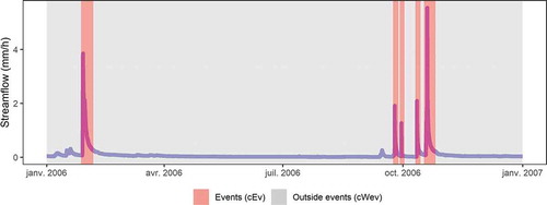
Figure 4 illustrates the streamflow time windows that are considered in the calculation of β_cEv and β_cWev.

Figure 4. Illustration of the streamflow time windows used to calculate the event bias per catchment and the bias outside periods with events per catchment. The hydrograph presented here corresponds to the Lergue River at Lodève (southern France)

A bounded version of these criteria, β^b, is calculated in order to facilitate comparison of results between catchments (Mathevet et al. 2006), as the bias can tend towards very large values when streamflow is overestimated. The highly skewed distribution introduces difficulties in interpreting mean values and dispersion over a set of criteria values.

(5) ${\beta }^b=\frac{\beta }{\beta +2}\in \left[-1,1\right]$(5)

Table 2 presents the corresponding values of β for some values of β^b. Negative values indicate underestimation of observed streamflow, and positive values indicate overestimation of observed streamflow by the model. A value of 0 indicates that there is no bias. We then refined the level of focus by investigating the seasonality of each bias. To calculate the four seasonal biases (β_ts, β_ev, β_cEv and β_cWev), we assumed that a flood occurred in a given season if the time of peak was in that season.

Table 2. Correspondence between bias (β) and bounded bias (β^b) values

β^b	β	β	β
−1	−1	0	0
−0.6	−0.75	0.11	0.25
−0.33	−0.5	0.2	0.5
−0.14	−0.25	0.33	1
−0.05	−0.1	0.5	2

3.3 Linking flood characteristics with model bias

Considering the catchments on which we identified patterns of seasonal event bias, we performed a univariate analysis between event bias and certain flood characteristics. Table 3 lists the characteristics considered in this analysis. Precipitation events were attributed to each flood event. The time window of a precipitation event was set as the time window of the corresponding flood event negatively shifted by the time of concentration of the catchment (see Table 1). The soil wetness index (SWI), calculated by the ISBA surface model (Thirel et al. 2010a, 2010b, Coustau et al. 2015), was used as an indicator of the soil moisture condition of the catchments. It is defined by Barbu et al. (2011) as follows:

(6) $SWI=\frac{w_{tot}-w_{wilt}}{w_{fc}-w_{wilt}}$(6)

Table 3. List of the relative characteristics used for the univariate analysis. All characteristics are expressed as percentages

Relative maximum hourly precipitation of the event

Relative maximum event streamflow (or peak flow)

Relative mean SWI index of the event

(ISBA model; Thirel et al. 2010a, 2010b, Coustau et al. 2015)

Relative event runoff coefficient (Q/P)

Relative event duration

with w_tot being the root soil moisture, w_wilt the wilting point and w_fc the field capacity. We used the daily catchment-averaged SWI values. We calculated the mean SWI values of each event. Each characteristic was then divided by its corresponding catchment event average (over both sub-periods) to compare the variability of events within catchments. For example, the relative duration of an event is calculated by dividing its duration by the average event duration of the catchment.

4 Results

4.1 Overall model performance

Figure 5 shows the distributions of KGE values over the 229 catchments and calculated for the calibration and validation periods.

Figure 5. Distribution of GR5H-I performance in calibration and validation periods over 229 French catchments. The distributions are presented between the 5^th and 95^th percentiles

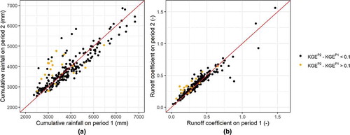
The first and third quartiles (Q₁ and Q₃) in calibration mode are between 0.90 and 0.95 in P1 and between 0.91 and 0.95 in P2. In validation mode, Q₁ and Q₃ are between 0.75 and 0.90 in P1 and between 0.79 and 0.91 in P2. As expected, the distributions show a drop in performance between the calibration and validation periods. The distribution of KGE values is more scattered in P1 than in P2. This can be partly explained by a change in the runoff coefficient and cumulative rainfall between P1 and P2 for some of the catchments in our dataset (see Fig. 6).

Figure 6. Difference of (a) cumulative rainfall and KGE; (b) runoff coefficient and KGE in validation mode between P1 and P2

The lowest KGE values in validation mode correspond to a few catchments located in the Mediterranean region. These results are consistent with previous nationwide studies with the GR models (e.g. Lobligeois et al. 2014, Ficchì et al. 2016, Poncelet et al. 2017). Crochemore et al. (2015) showed that KGE values between 0.66 and 0.90 are considered to represent good model performance according to expert judgement. We can therefore consider that the GR5H-I model yields good overall performance in our dataset.

4.2 Model bias on four levels of hydrograph disaggregation

We then refined the analysis and investigated whether the model was able to simulate the 2990 flood events in our catchment dataset. In this regard, the model bias was calculated considering the four levels of hydrograph disaggregation (Fig. 7) defined earlier to enable identification of compensations between streamflow periods, i.e. between periods of floods and mean and low flows.

Figure 7. Distribution of GR5H-I bias over 229 catchments and 2990 events. The bias (bounded) was calculated for four levels of hydrograph disaggregation. The distributions are presented between the 5^th and 95^th percentiles. Calculations were made with cross-validation values, i.e. using simulations on P1 and P2 obtained with the parameter sets optimized on P2 and P1, respectively

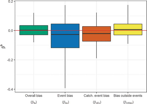
The median event bias (β_ev^b) of the GR5H-I model is equal to −0.03, and its distribution is left-skewed towards negative values. The distribution of catchment event bias (β_cEv^b) is similar to the distribution of event bias, with a median value of −0.02 and a lesser dispersion. When bias is calculated without taking the selected flood events into account (β_cWev^b), the median bias has a value of 0.01. The distribution is wider for positive values outside the interquartile range. The model bias calculated for the entire time series (β_ts^b) has a median value of 0.001 and a distribution similar to the distribution of β_cWev^b . The dispersion of the event bias is wider than the distribution of the three other biases. The dispersion of the bias calculated for the whole time series is narrower than the other distributions. Overall, these results show that there are compensations between periods where flood events occur and the rest of the hydrograph. The four bias criteria were also calculated in the calibration period and the results showed similar patterns (not shown here).

4.3 Seasonality of model bias

We investigated to what extent certain flood events are better reproduced by the model. As the seasonal variation of streamflow affects antecedent soil moisture conditions, it is a good indicator of the variability in flood characteristics across Metropolitan France. We therefore compared the four bias criteria with the seasonality of floods (Fig. 8(a–d)).

Figure 8. Seasonality of GR5H-I bias over 229 catchments and 2990 events. The bias (bounded) was calculated on four levels of hydrograph disaggregation. The distributions are presented between the 5^th and 95^th percentiles. Calculations were made with cross-validation values. n_c is the related number of catchments and n_ev is the related number of flood events. Part (c) shows the seasonal distributions for all catchments

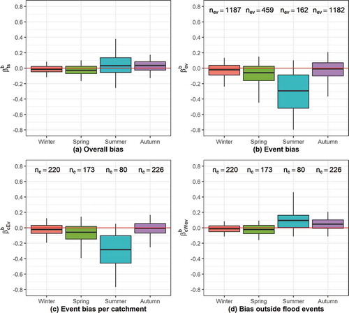
Figure 8(b) shows that more than 75% of the observed summer floods were underestimated by the GR5H-I model. The distribution of event bias shows that the underestimation associated with summer events is much larger than with the other flood events of our dataset. Floods that occur in winter and autumn were less underestimated by the model. The distribution of bias across summer events is wider than the bias calculated for the simulations of the other flood events. The largest overestimations of floods were for autumn events. Large underestimations of summer events explain the skewness of the distribution of GR5H-I event bias presented in Fig. 7. Figure 8(c) shows that the seasonal trend of model event bias is also an intra-catchment pattern. The distributions are less dispersed but the tendency remains similar. The seasonal distribution of model bias calculated in the entire hydrograph exhibits a different pattern (Fig. 8(a)). Summer and autumn bias distributions have positive median values. Winter and spring distributions are similar to the distributions in Fig. 8(b) and (c) but with a narrower dispersion. When the bias is calculated without flood events (Fig. 8(d)), winter and summer distributions remain similar to the time series bias. Summer and autumn periods are overestimated for 75% of the corresponding catchments. These results indicate compensation between periods of flood events and periods where there are no flood events in summer and spring. Event bias seems to affect winter and spring periods less in our dataset.

Figure 9(a–h) presents the GR5H-I simulations of eight floods that occurred in tributaries of three major French rivers, the Rhône (Doux and Ardèche tributaries), Seine and Garonne rivers.

Figure 9. Examples of simulations of summer floods compared with floods that occurred in other seasons. Simulations of GR5H-I are in validation mode. β_ev is the flood event bias. β_ts and KGE are the bias and KGE index, respectively, calculated for the entire corresponding validation period

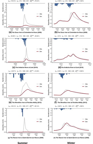
The GR5H-I model failed to reproduce the volumes of the summer events (Fig. 9(a, c, e, g)), whereas it was able to reproduce the volumes of four floods that occurred in other seasons (Fig. 9(b, d, f, h)). The GR5H-I model yielded reasonable performance for the rest of the time series, as assessed by the KGE index.

4.4 Relationship between event bias and flood characteristics

Based on the 80 catchments where flood events occur in summer, we investigated the relationships between model event bias and various flood characteristics. Figure 10 presents the univariate analysis of the links between GR5H-I bias on floods and flood characteristics.

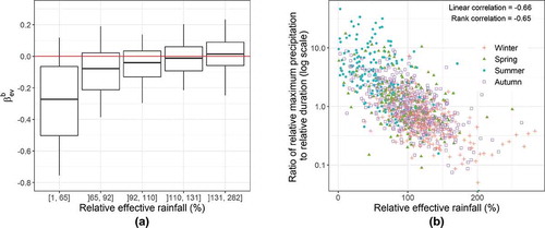
Figure 10. (a) to (e) present the results of a univariate analysis of the relationships between flood characteristics and event bias β_ev^b for 80 catchments in which floods occur in summer. Each characteristic class contains approximatively 211 events. The flood characteristics presented are relative to the mean flood characteristics of the corresponding catchment. (b) is the linear correlation matrix between the relative flood characteristics

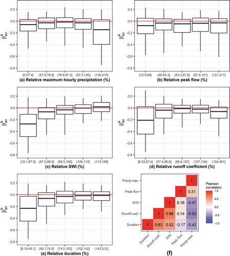
Figure 10(a) shows that GR5H-I bias is lower for flood events for which the maximum hourly precipitation exceeds 130% of the mean of maximum event precipitation. Figure 10(b) shows that there is no clear relationship between event peak flow and model bias. Large underestimations of flood volumes are associated with low SWI index values (Fig. 10(c)) and short-duration events (Fig. 10(e)). Interestingly, low runoff coefficient values are associated with larger underestimations (Fig. 10(d)). As expected, the highest correlation between flood characteristics is between the SWI index and the runoff coefficient (Fig. 10(f)). The runoff coefficient is also positively correlated with flood duration and negatively correlated with maximum precipitation. These results indicate that the largest underestimations of flood volumes by the GR5H-I model are for short floods occurring in summer under low soil moisture conditions and when high-intensity precipitation events take place.

5 Discussion

Our analysis was based on bias calculations considering different periods of the hydrograph to evaluate the capacity of a conceptual rainfall-runoff model to simulate flood events. By refining the time window of analysis and by using the seasonality of streamflow water balance as a proxy of flood variability, we found patterns of seasonal model bias. These patterns of seasonal model bias are linked to soil moisture conditions and specific characteristics associated with the flood events. We now discuss how informative this analysis can be in light of other existing diagnostics.

5.1 How informative is the KGE index for summer events?

We have shown that calculating the model bias for different streamflow time windows enabled us to highlight compensations between high-flow periods and periods without floods as well as situations where the model was not able to simulate flood volumes. One may wonder whether these results could be obtained with aggregated statistics such as the KGE criterion. In other words, we wanted to know whether the catchments in which the model yielded low KGE values are the catchments in which the summer floods were underestimated. First, the comparison between overall bias and event bias showed differences in the ability of the GR5H-I model to simulate the global water balance and to simulate flood volumes. One reason may be the low water volumes associated with summer events compared with the other floods in our dataset (see Fig. 2). Mizukami et al. (2019) reported similar results when investigating differences in annual peak flow simulations. They showed that improving streamflow bias did not always result in better simulation of flood magnitudes. Furthermore, the results presented in Fig. 11 demonstrate that there is no clear relationship between aggregated KGE values and event bias for catchments in which summer floods occur.

Figure 11. GR5H-I summer event bias per catchment plotted against KGE values for catchments where flood events occurred in summer

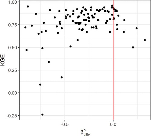
This is consistent with the findings of Brunner et al. (2020), who showed that while the KGE index integrates a flow bias component, it does not explicitly account for high-flow values. These results are also in line with the study by Mathevet et al. (2020), who found that two conceptual models yielded similar results when looking at criteria calculated for the whole time series but found differences in the ability of the model to capture short-term processes when investigating criteria calculated for specific sub-periods. These results show that investigating the seasonality of model bias considering different streamflow time windows can offer new information on the ability of a model to simulate specific flood events.

5.2 On the relevance of event and seasonality analyses to improve simulation of floods

To investigate seasonal patterns in model errors, other hydrological signatures could be based on the hydrological regime (or 365-d rolling mean, e.g. Mathevet et al. 2020) or the flow duration curve (e.g. Yilmaz et al. 2008). However, as presented in section 4.3, the seasonal model bias did not highlight underestimations by the model of flood events observed in summer. The investigation of specific events along with seasonality clearly enabled the identification of patterns in model errors. Another way to identify these patterns would be to derive the flow duration curve in summer periods and calculate differences above the 80^th percentile. But the advantage of flood event selection and analysis lies in the possibility to investigate links to various flood characteristics. Floods can have very different seasonal triggers affecting antecedent soil moisture conditions at different time scales (Blöschl et al. 2013, Berghuijs et al. 2014). Therefore, fast processes are not always considered in overall performance analyses. The seasonality of floods is a good indicator of flood triggers in metropolitan France. Our results showed that combining event analysis with streamflow seasonality analysis can help to identify where a conceptual model fails to reproduce flood volumes even when the model yields an aggregated performance considered to be reasonable.

5.3 First-order factors controlling simulation errors

One of the underlying ideas behind diagnosing a model is to be able to identify where model improvement is needed. In the case of the GR5H-I model, our results showed a clear seasonal pattern with an unbiased estimation of floods except in summer, where there is a clear underestimation signal. A central question remains regarding the first-order factors leading to the identified deficiency. Model deficiency can be related to parameter estimation, either because of the choice of objective function (e.g. Mizukami et al. 2019, Brunner et al. 2020) or because of data uncertainty (i.e. wrong parameterization because of uncertainty in forcings or streamflows; see e.g. Beven 2016). However, structural deficiencies may be the underlying cause in the case of our model, as its parsimonious structure could limit its ability to reproduce specific processes occurring in summer, where short-duration processes can take place, such as high-intensity precipitation events. We have seen that this is especially the case under low soil moisture conditions. Furthermore, Fig. 12(a) indicates that the simulation of effective rainfall by the GR5H-I model partly explains the large underestimations of some of the flood events. When the simulation of effective rainfall is low compared with the other floods of a catchment, the model tends to underestimate the flood volume. Figure 12(b) presents the relationship between a measure of precipitation intensity and flashiness of the catchment response and GR5H-I simulation of event effective rainfall. Low values of effective rainfall are associated with short-duration events with high precipitation intensity (large y-axis values) and mostly for late spring, summer and early autumn events.

Figure 12. (a) Relationship between GR5H-I simulation of event effective rainfall and event bias (each class contains approximatively 211 events). (b) Relationship between GR5H-I simulation of event effective rainfall and precipitation intensity relative to event duration. The results are for 1054 events that took place in 80 catchments in which floods can occur in summer

Whatever parameter set is chosen, models sometimes do not have the structural ability to reproduce an observed flood. This explanation is consistent with the findings of Mathevet et al. (2020), who reported that the shorter the sub-period of evaluation, the greater the difference in performance between the MRX model and the GRX model (similar to GR5H-I). They concluded that MRX is better able to reproduce short-term processes than GRX because of the more complex structure of the former. The lumped spatial configuration could also be the restraining factor explaining the deficiencies identified, since spatial interactions between precipitations and soil wetness have impacts on flood generation (Tarasova et al. 2020). Short-duration events with high precipitation intensity are sometimes subject to large uncertainties in the input precipitation data (e.g. Zoccatelli et al. 2011, Ruiz-Villanueva et al. 2012, Zhang et al. 2017). If the total amount of rainfall is underestimated during an event, the model cannot simulate the required amount of effective rainfall. This could explain, to some extent, that the model does not perform well on such events. Whatever the first-order factor is, the present methodology, by establishing a finer benchmark for high-flow simulations, helped reveal the difficulties involved in modelling specific flood events. This is particularly relevant to reduce model structure uncertainty and therefore to improve the predictive capability of our model. This work will contribute to future improvements of the GR5H-I model.

6 Conclusion

In this study, we proposed an approach to diagnose the quality of floods simulated by a conceptual rainfall-runoff model over a large set of catchments and flood events. Starting from overall performance criteria calculated for the whole time series, our methodology consisted in computing model bias for selected flood events and looking for seasonal trends and compensations between streamflow periods. From these seasonal patterns, we aimed to link the model bias to certain flood characteristics. We found that while the model yielded reasonable performance for the dataset in terms of aggregated statistics, patterns in model errors were revealed when investigating performance across selected flood events. Using seasonality as an indicator of the variability of flood characteristics enabled us to identify situations where the GR5H-I model did not manage to reproduce the observed flood volumes. We found that the summer events of our dataset were associated with systematic underestimations by the GR5H-I model. Short-duration processes, such as high-intensity precipitation events, associated with low soil moisture conditions are not explicitly taken into account in the structure of the GR5H-I model. For these specific events, this results in a too-low simulation of effective rainfall and therefore underestimation of flood volumes. However, these simulation errors were not detected when considering the KGE index calculated for the entire streamflow time series. By examining both the seasonality of model bias and different streamflow time windows, we have identified compensations between flood events and the rest of the hydrograph in summer and autumn.

Overall, this study confirmed the limitations of using criteria computed on the whole time series to evaluate model performance in simulating high-flow events, even when these criteria are known to be biased towards high flows. The seasonality of streamflow was found to be an indicator of the ability of the GR5H-I model to simulate specific floods that occurred in some of the catchments of our dataset. It enabled us to refine the analyses and look for links to flood characteristics for these catchments. Future developments of the model could focus on improving the calculation of effective rainfall by accounting for summer flood-generating processes. This could be achieved by better considering the spatial variability of rainfall (e.g. Lobligeois et al. 2014, Loritz et al. 2021) or by taking precipitation intensity into account (e.g. Peredo et al. 2021). Multi-objective calibration could also lead to an improved identification of the parameter sets (e.g. Monteil et al. 2020), using, for example, objective functions that were found to be more suited for flood simulation (e.g. Mizukami et al. 2019).

In this study, we focused on model bias because we considered it a first-order property of model errors. Another perspective on our work could be to further analyse model simulations within a multicriteria assessment framework so as to cover more aspects of model performance (Willems 2009). Also, data uncertainty was not considered for model parameterization or for streamflow result analyses, although it can have an impact on model parameterization and interpretation of model errors (Beven 2016). Finally, further tests on other catchments, such as dry or arid catchments (e.g. in Australia), could improve the generalizability of our results.

Acknowledgements

The authors thank Météo-France and Banque HYDRO for providing the climatic and hydrological data, respectively. We also thank Pierre-André Garambois for reviewing an earlier version of the manuscript. Finally, we thank the Associate Editor, Andrea Petroselli, and three anonymous referees for their very constructive comments that helped us improve the paper.

Disclosure statement

No potential conflict of interest was reported by the authors.

Correction Statement

This article has been republished with minor changes. These changes do not impact the academic content of the article.

Additional information

Funding

This work was supported by Ministère de la Transition écologique, which provided financial support to the PhD grant of the first author.

Appendix.

Equations of the GR5H-I model

Here we provide the main equations (integrated over the time step) of the GR5H-I model along with a diagram that depicts the model conceptual storages and fluxes (Fig. A1). Definitions of the variables and parameters are given in Tables A1 and Tables A2, respectively. More information about the model can be found in Le Moine (2008), Lobligeois (2014) and Ficchì et al. (2019).

The following equations provide the detailed computations of the various internal and output variables of the model on a given time step. The sequence can be repeated within a loop to compute a time series of simulated streamflow. Before these computations start, the ordinates of the unit hydrograph must be calculated (see Equations A9 and A10).

Interception store:

At current time step $k$, evapotranspiration from the interception store $E_i$ is calculated from potential evapotranspiration input $E$, precipitation input $P$ and antecedent interception store level $I$:

(A1) $E_i\left(k\right)=min\left(E\left(k\right),P\left(k\right)+I\left(k-1\right)\right)$(A1)

Then, net rainfall is calculated as follows:

(A2) $P_{th}\left(k\right)=max\left[0,P\left(k\right)-\left(I_{max}-I\left(k-1\right)\right)-E_i\left(k\right)\right]$(A2)

The interception store level is then updated as follows:

(A3) $I\left(k\right)=I\left(k-1\right)+P\left(k\right)-E_i\left(k\right)-P_{th}\left(k\right)$(A3)

Production store:

The part of net rainfall that fills the production store depends on the antecedent production store level and the net rainfall:

(A4) $P_s\left(\mathrm{k}\right)=\frac{X_1\left(1-{\left(\frac{S\left(k-1\right)}{X_1}\right)}^2\right)tanh\left(\frac{P_{th}\left(k\right)}{X_1}\right)}{1+\frac{S\left(k-1\right)}{X_1}tanh\left(\frac{P_{th}\left(k\right)}{X_1}\right)}$(A4)

In case $E\left(k\right)-E_i\left(k\right)$ is greater than zero, evapotranspiration from the production store occurs and depends on the antecedent production store level:

(A5) $E_s\left(\mathrm{k}\right)=\frac{S\left(k-1\right).\left(2-\frac{S\left(k-1\right)}{X_1}\right)tanh\left(\frac{\mathrm{E}\left(\mathrm{k}\right)-E_i\left(k\right)}{X_1}\right)}{1+\left(1-\frac{S\left(k-1\right)}{X_1}\right)tanh\left(\frac{\mathrm{E}\left(\mathrm{k}\right)-E_i\left(k\right)}{X_1}\right)}$(A5)

The production store level is then updated as follows:

(A6) $S^{\ast }\left(k\right)=S\left(k-1\right)+P_s\left(k\right)-E_s\left(k\right)$(A6)

Percolation from the production store is calculated as:

(A7) $Perc\left(k\right)=S^{\ast }\left(k\right).\left\{1-{\left[1+{\left(\frac{4}{21}.\frac{S\left(k\right)}{X_1}\right)}^4\right]}^{-\frac{1}{4}}\right\}$(A7)

(A8) $S\left(k\right)=S^{\ast }\left(k\right)-Perc\left(k\right)$(A8)

Unit hydrograph (UH):

The S-curve along time t is defined independently from the current time step:

(A9) $\left\{\begin{array}{c}0,t<0\\ -\frac{1}{2}.{\left(\frac{t}{X_4}\right)}^{1.25},0<t<X_4\\ 1-\frac{1}{2}.{\left(2-\frac{t}{X_4}\right)}^{1.25},X_4<t<2.X_4\\ 1,t\ge 2.X_4\end{array}\right.$(A9)

The resulting unit hydrograph ordinates are calculated by:

(A10) $UH\left(j\right)=SH\left(j\right)-SH\left(j-1\right)$(A10)

where j is an integer between 1 and the maximum number of unit hydrograph ordinates (n).

The unit hydrograph ordinates are used to calculate the outflow from the unit hydrograph to the routing store at the current time step:

(A11) $Q_9\left(k\right)=\frac{9}{10}.\sum _{j=1}^{n}UH\left(j\right).P_r\left(k-j+1\right)$(A11)

and the outflow from the unit hydrograph to the direct branch:

(A12) $Q_1\left(k\right)=\frac{1}{10}.\sum _{j=1}^{n}UH\left(j\right).P_r\left(k-j+1\right)$(A12)

Exchange function:

An intercatchment exchange flow is then added (or released) to (or from) both outflows depending on the antecedent routing store level. The potential intercatchment semi-exchange is calculated as follows:

(A13) $F\left(k\right)=X_2\left(\frac{R\left(k-1\right)}{X_3}-X_5\right)$(A13)

Routing store:

The routing store level is updated as follows:

(A14) $R^{\ast }\left(k\right)=max[0,R\left(k-1\right)+Q_9\left(k\right)+F\left(k\right)$(A14)

The outflow from the routing store is then calculated as:

(A15) $Q_r\left(k\right)=R^{\ast }\left(k\right).\left\{1-{\left[1+{\left(\frac{R\left(k\right)}{X_3}\right)}^4\right]}^{-\frac{1}{4}}\right\}$(A15)

(A16) $R\left(k\right)=R^{\ast }\left(k\right)-Q_r\left(k\right)$(A16)

The outflow from the direct branch is expressed as:

(A17) $Q_d\left(k\right)=max\left[0,Q_1\left(k\right)+F\left(k\right)\right]$(A17)

Finally, the simulated streamflow is calculated as:

(A18) $Q\left(k\right)=Q_r\left(k\right)+Q_d\left(k\right)$(A18)

Table A1. List of the variables of GR5H-I expressed for a given time step (mm or mm/h)

Notation	Definition
$E$	Potential evapotranspiration input
$P$	Precipitation input
$E_n$	Net evapotranspiration
$E_i$	Evapotranspiration from interception store
$Imax$	Interception store capacity
$I$	Interception store level
$P_{th}$	Net rainfall from interception store
$E_s$	Evapotranspiration from production store
$P_s$	Part of net rainfall that fills the production store
$S^{\ast }$	Temporary level of the production store
$S$	Production store level
$Perc$	Percolation from production store
$P_r$	Effective rainfall
$Q9$	Part of the unit hydrograph outflow that fills the routing store
$Q1$	Part of the unit hydrograph outflow that does not fill the routing store
$F$	Potential intercatchment semi-exchange
	Outflow from the routing store
$Q_d$	Outflow from the direct branch
$R^{\ast }$	Temporary level of the routing store
$R$	Routing store level
$Q$	Simulated streamflow

Table A2. List of the free parameters of GR5H-I

Notation	Definition	Unit
$X_1$	Production store capacity	mm
$X_2$	Intercatchment exchange coefficient	mm/h
$X_3$	Routing store capacity	mm
$X_4$	Unit hydrograph time constant	h
$X_5$	Intercatchment exchange threshold	-

Figure A1. Diagram of the GR5H-I model (modified from Le Moine 2008, Ficchì et al. 2019)

References

- Andréassian, V., et al., 2009. HESS opinions “crash tests for a standardized evaluation of hydrological models”. Hydrology and Earth System Sciences, 13, 1757–1764. doi:10.5194/hess-13-1757-2009.
- Andréassian, V., et al., 2014. Seeking genericity in the selection of parameter sets: impact on hydrological model efficiency. Water Resources Research, 50, 8356–8366. doi:10.1002/2013WR014761.
- Barbu, A.L., et al., 2011. Assimilation of Soil Wetness Index and Leaf Area Index into the ISBA-A-gs land surface model: grassland case study. Biogeosciences, 8, 1971–1986. doi:10.5194/bg-8-1971-2011.
- Bennett, N.D., et al., 2013. Characterising performance of environmental models. Environmental Modelling and Software, 40, 1–20. doi:10.1016/j.envsoft.2012.09.011.
- Berghuijs, W.R., et al., 2014. Patterns of similarity of seasonal water balances: a window into streamflow variability over a range of time scales. Water Resources Research, 50, 5638–5661. doi:10.1002/2014WR015692.
- Berthet, L., et al., 2009. How crucial is it to account for the antecedent moisture conditions in flood forecasting? Comparison of event-based and continuous approaches on 178 catchments. Hydrology and Earth System Sciences, 13 (6), 819–831. doi:10.5194/hess-13-819-2009.
- Berthet, L., 2010. Flood forecasting at the hourly time step: towards a better assimilation of streamflow information in a hydrological model. PhD Thesis (in French). AgroParisTech.
- Beven, K.J., 2016. Facets of uncertainty: epistemic uncertainty, non-stationarity, likelihood, hypothesis testing, and communication. Hydrological Sciences Journal, 61, 1652–1665. doi:10.1080/02626667.2015.1031761.
- Blöschl, G., et al., 2013. Runoff prediction in ungauged basins: synthesis across processes places and scales. Cambridge University Press. doi:10.1017/CBO9781139235761.
- Borah, D.K., et al., 2007. Storm event and continuous hydrologic modeling for comprehensive and efficient watershed simulations. Journal of Hydrologic Engineering, 12 (6), 605–616. doi:10.1061/(ASCE)1084-0699(2007)12:6(605).
- Brunner, M.I., et al., 2020. Flood hazard and change impact assessments may profit from rethinking model calibration strategies. preprint. Catchment hydrology/Modelling Approaches. doi:10.5194/hess-2020-192.
- Butts, M.B., et al., 2004. An evaluation of the impact of model structure on hydrological modelling uncertainty for streamflow simulation. Journal of Hydrology, 298, 242–266. doi:10.1016/j.jhydrol.2004.03.042.
- Carsell, K.M., Pingel, N.D., and Ford, D.T., 2004. Quantifying the benefit of a flood warning system. Natural Hazards Review, 5, 131–140. doi:10.1061/(ASCE)15276988(2004)5:3(131).
- Clark, M.P., et al., 2008. Framework for Understanding Structural Errors (FUSE): a modular framework to diagnose differences between hydrological models. Water Resources Research, 44, W00B02+. doi:10.1029/2007WR006735.
- Coron, L., et al., 2012. Crash testing hydrological models in contrasted climate conditions: an experiment on 216 Australian catchments. Water Resources Research, 48. doi:10.1029/2011WR011721.
- Coron, L., et al., 2017. The Suite of lumped GR hydrological models in an R package. Environmental Modelling and Software, 94, 166–171. doi:10.1016/j.envsoft.2017.05.002.
- Coron, L., et al., 2021. airGR: suite of GR hydrological models for precipitation-runoff modelling. R package version 1.6.9.27. doi:10.15454/EX11NA. Available from: https://CRAN.R-project.org/package=airGR/.
- Coustau, M., et al., 2015. Impact of improved meteorological forcing, profile of soil hydraulic conductivity and data assimilation on an operational Hydrological Ensemble Forecast System over France. Journal of Hydrology, 525, 781–792. doi:10.1016/j.jhydrol.2015.04.022.
- Crochemore, L., et al., 2015. Comparing expert judgement and numerical criteria for hydrograph evaluation. Hydrological Sciences Journal, 60, 402–423. doi:10.1080/02626667.2014.903331.
- de Boer-Euser, T., et al., 2017. Looking beyond general metrics for model comparison – lessons from an international model intercomparison study. Hydrology and Earth System Sciences, 21, 423–440. doi:10.5194/hess-21-423-2017.
- Delaigue, O., et al., 2020. Database of watershed-scale hydroclimatic observations in France. France: INRAE, HYCAR Research Unit, Hydrology group, Antony. https://webgr.inrae.fr/base-de-donnees.
- Donnelly, C., Andersson, J.C., and Arheimer, B., 2016. Using flow signatures and catchment similarities to evaluate the E-HYPE multi-basin model across Europe. Hydrological Sciences Journal, 61, 255–273. doi:10.1080/02626667.2015.1027710.
- Ducharne, A., 2009. Reducing scale dependence in TOPMODEL using a dimensionless topographic index. Hydrology and Earth System Sciences, 13, 2399–2412. doi:10.5194/hess-13-2399-2009.
- Euser, T., et al., 2013. A framework to assess the realism of model structures using hydrological signatures. Hydrology and Earth System Sciences, 17, 1893–1912. doi:10.5194/hess-17-1893-2013.
- Ficchì, A., 2017. An adaptive hydrological model for multiple time-steps: diagnostics and improvements based on fluxes consistency. Ph.D. thesis. Paris: UPMC.
- Ficchì, A., Perrin, C., and Andréassian, V., 2016. Impact of temporal resolution of inputs on hydrological model performance: an analysis based on 2400 flood events. Journal of Hydrology, 538, 454–470. doi:10.1016/j.jhydrol.2016.04.016.
- Ficchì, A., Perrin, C., and Andréassian, V., 2019. Hydrological modelling at multiple sub-daily time steps: model improvement via flux-matching. Journal of Hydrology, 575, 1308–1327. doi:10.1016/j.jhydrol.2019.05.084.
- Fowler, K.J.A., et al., 2016. Simulating runoff under changing climatic conditions: revisiting an apparent deficiency of conceptual rainfall-runoff models. Water Resources Research, 52, 1820–1846. doi:10.1002/2015WR018068.
- Gnann, S.J., Howden, N.J.K., and Woods, R.A., 2020. Hydrological signatures describing the translation of climate seasonality into streamflow seasonality. Hydrology and Earth System Sciences, 24, 561–580. doi:10.5194/hess-24-561-2020.
- Grimaldi, S., et al., 2020. Continuous hydrologic modelling for design simulation in small and ungauged basins: a step forward and some tests for its practical use. Journal of Hydrology, 125664. doi:10.1016/j.jhydrol.2020.125664.
- Gupta, H.V., et al., 2009. Decomposition of the mean squared error and NSE performance criteria: implications for improving hydrological modelling. Journal of Hydrology, 377, 80–91. doi:10.1016/j.jhydrol.2009.08.003.
- Gupta, H.V., et al., 2014. Large-sample hydrology: a need to balance depth with breadth. Hydrology and Earth System Sciences, 18, 463–477. doi:10.5194/hess-18-463-2014.
- Gupta, H.V., Wagener, T., and Liu, Y., 2008. Reconciling theory with observations: elements of a diagnostic approach to model evaluation. Hydrological Processes, 22, 3802–3813. doi:10.1002/hyp.6989.
- Gustard, A., Bullock, A., and Dixon, J., 1992. Low flow estimation in the United Kingdom. Institute of Hydrology. http://nora.nerc.ac.uk/id/eprint/6050/1/IH_108.pdf
- Hallegatte, S., 2012. A cost effective solution to reduce disaster losses in developing countries: hydroMeteorological Services, early warning, and evacuation. The World Bank. doi:10.1596/1813-9450-6058.
- Hapuarachchi, H.A.P., Wang, Q.J., and Pagano, T.C., 2011. A review of advances in flash flood forecasting. Hydrological Processes, 25, 2771–2784. doi:10.1002/hyp.8040.
- Hrachowitz, M., et al., 2014. Process consistency in models: the importance of system signatures, expert knowledge, and process complexity. Water Resources Research, 50, 7445–7469. doi:10.1002/2014WR015484.
- Jain, S.K., et al., 2018. A Brief review of flood forecasting techniques and their applications. International Journal of River Basin Management, 16, 329–344. doi:10.1080/15715124.2017.1411920.
- Javelle, P., et al., 2010. Flash flood warning at ungauged locations using radar rainfall and antecedent soil moisture estimations. Journal of Hydrology, 394, 267–274. doi:10.1016/j.jhydrol.2010.03.032.
- Jeuland, M., et al., 2019. The economic impacts of water information systems: a systematic review. Water Resources and Economics, 26, 100128. doi:10.1016/j.wre.2018.09.001
- Kim, H. and Lee, S., 2014. Assessment of a seasonal calibration technique using multiple objectives in rainfallrunoff analysis. Hydrological Processes, 28, 2159–2173. doi:10.1002/hyp.9785.
- Klemeš, V., 1986. Operational testing of hydrologic simulation models. Hydrological Sciences Journal, 31 (1), 13–24. doi:10.1080/02626668609491024.
- Knoben, W.J.M., et al., 2020. A brief analysis of conceptual model structure uncertainty using 36 models and 559 catchments. Water Resources Research, 56. doi:10.1029/2019WR025975.
- Lane, R.A., et al., 2019. Benchmarking the predictive capability of hydrological models for river flow and flood peak predictions across over 1000 catchments in Great Britain. Hydrology and Earth System Sciences, 23, 4011–4032. doi:10.5194/hess-23-4011-2019.
- Le Moine, N., 2008. Le bassin versant de surface vu par le souterrain: une voie d’amélioration des performances et du réalisme des modèles pluie-débit? Ph.D. thesis. UPMC, Cemagref.
- Leleu, I., et al., 2014. La refonte du système d’information national pour la gestion et la mise à disposition des données hydrométriques. La Houille Blanche, 25–32. doi:10.1051/lhb/2014004.
- Lobligeois, F., 2014. Mieux connaître la distribution spatiale des pluies améliore-t-il la modélisation des crues? Ph.D. thesis. Paris: UPMC, AgroParisTech.
- Lobligeois, F., et al., 2014. When does higher spatial resolution rainfall information improve streamflow simulation? An evaluation using 3620 flood events. Hydrology and Earth System Sciences, 18, 575–594. doi:10.5194/hess-18-575-2014.
- Loritz, R., et al., 2021. The role and value of distributed precipitation data in hydrological models. Hydrology and Earth System Sciences, 25, 147–167. doi:10.5194/hess-25-147-2021.
- Massmann, C., 2020. Identification of factors influencing hydrologic model performance using a top-down approach in a large number of U.S. catchments. Hydrological Processes, 34, 4–20. doi:10.1002/hyp.13566.
- Mathevet, T., et al., 2006. A bounded version of the Nash-Sutcliffe criterion for better model assessment on large sets of basins. IAHS-AISH Publication, 307, 211.
- Mathevet, T., et al., 2020. Assessing the performance and robustness of two conceptual rainfall-runoff models on a worldwide sample of watersheds. Journal of Hydrology, 585, 124698. doi:10.1016/j.jhydrol.2020.124698.
- McMillan, H., Booker, D., and Cattoën, C., 2016. Validation of a national hydrological model. Journal of Hydrology, 541, 800–815. doi:10.1016/j.jhydrol.2016.07.043.
- McMillan, H., Westerberg, I., and Branger, F., 2017. Five guidelines for selecting hydrological signatures. Hydrological Processes, 31, 4757–4761. doi:10.1002/hyp.11300.
- Melsen, L.A., et al., 2018. Mapping (dis)agreement in hydrologic projections. Hydrology and Earth System Sciences, 22, 1775–1791. doi:10.5194/hess-22-1775-2018.
- Michel, C., 1991. Hydrologie appliquée aux petits bassins ruraux. Antony, France: Cemagref.
- Mizukami, N., et al., 2019. On the choice of calibration metrics for “high-flow” estimation using hydrologic models. Hydrology and Earth System Sciences, 23, 2601–2614. doi:10.5194/hess-23-2601-2019.
- Monteil, C., et al., 2020. Multi-objective calibration by combination of stochastic and gradient-like parameter generation rules – the caRamel algorithm. Hydrology and Earth System Sciences, 24, 3189–3209. doi:10.5194/hess-24-3189-2020.
- Muleta, M.K., 2012. Improving model performance using season-based evaluation. Journal of Hydrologic Engineering, 17, 191–200. doi:10.1061/(ASCE)HE.1943-5584.0000421.
- Nash, J.E. and Sutcliffe, J.V., 1970. River flow forecasting through conceptual models, Part I: a discussion of principles. Journal of Hydrology, 27 (3), 282–290. doi:10.1016/0022-1694(70)90255-6.
- Nicolle, P., et al., 2014. Benchmarking hydrological models for low-flow simulation and forecasting on French catchments. Hydrology and Earth System Sciences, 18, 2829–2857. doi:10.5194/hess-18-2829-2014.
- Oudin, L., et al., 2005. Which potential evapotranspiration input for a lumped rainfall–runoff model?: Part 2—Towards a simple and efficient potential evapotranspiration model for rainfall–runoff modelling. Journal of Hydrology, 303, 290–306. doi:10.1016/j.jhydrol.2004.08.026.
- Oudin, L., et al., 2006. Dynamic averaging of rainfall-runoff model simulations from complementary model parameterizations. Water Resources Reasearch, 42. doi:10.1029/2005WR004636.
- Pagano, T.C., et al., 2014. Challenges of operational river forecasting. Journal of Hydrometeorology, 15, 1692–1707. doi:10.1175/JHM-D-13-0188.1.
- Pappenberger, F., et al., 2016. Hydrological ensemble prediction systems around the globe. In: Q. Duan, et al., eds. Handbook of hydrometeorological ensemble forecasting. Berlin, Heidelberg: Springer Berlin Heidelberg, 1–35. doi:10.1007/978-3-642-40457-3_47-1.
- Peredo, D., et al., 2021. Investigating hydrological model versatility to simulate extreme flood events. Hydrological Sciences Journal, In Review.
- Perrin, C., et al., 2008. Discrete parameterization of hydrological models: evaluating the use of parameter sets libraries over 900 catchments. Water Resources Research, 44. doi:10.1029/2007WR006579.
- Perrin, C., Michel, C., and Andréassian, V., 2001. Does a large number of parameters enhance model performance? Comparative assessment of common catchment model structures on 429 catchments. Journal of Hydrology, 242, 275–301. doi:10.1016/S0022-1694(00)00393-0.
- Poncelet, C., et al., 2017. Process-based interpretation of conceptual hydrological model performance using a multinational catchment set. Water Resources Research, 53, 7247–7268. doi:10.1002/2016WR019991.
- Roundy, J.K., Duan, Q., and Schaake, J., 2018. Hydrological predictability, scales, and uncertainty issues. In: Q. Duan, et al., eds. Handbook of hydrometeorological ensemble forecasting. Berlin, Heidelberg: Springer, 1–29. doi:10.1007/978-3-642-40457-3_8-1.
- Ruiz-Villanueva, V., et al., 2012. Extreme flood response to short-duration convective rainfall in South-West Germany. Hydrology and Earth System Sciences, 16, 1543–1559. doi:10.5194/hess-16-1543-2012.
- Sauquet, E., Gottschalk, L., and Krasovskaia, I., 2008. Estimating mean monthly runoff at ungauged locations: an application to France. Hydrology Research, 39, 403–423. doi:10.2166/nh.2008.331.
- Schaefli, B. and Gupta, H.V., 2007. Do Nash values have value? Hydrological Processes, 21, 2075–2080. doi:10.1002/hyp.6825.
- Seibert, J., 2001. On the need for benchmarks in hydrological modelling. Hydrological Processes, 15, 1063–1064. doi:10.1002/hyp.446.
- Seibert, J., et al., 2018. Upper and lower benchmarks in hydrological modelling. Hydrological Processes, 32, 1120–1125. doi:10.1002/hyp.11476.
- Shafii, M. and Tolson, B.A., 2015. Optimizing hydrological consistency by incorporating hydrological signatures into model calibration objectives. Water Resources Research, 51, 3796–3814. doi:10.1002/2014WR016520.
- Stanić, M., et al., 2018. Extreme flood reconstruction by using the 3DNet platform for hydrological modelling. Journal of Hydroinformatics, 20 (4), 766–783. doi:10.2166/hydro.2017.050.
- Stephens, C.M., Johnson, F.M., and Marshall, L.A., 2018. Implications of future climate change for event-based hydrologic models. Advances in Water Resources, 119, 95–110. doi:10.1016/j.advwatres.2018.07.004.
- Tabary, P., et al., 2012. A 10-year (1997–2006) reanalysis of quantitative precipitation estimation over France: methodology and first results. IAHS Publication, 351, 255–260.
- Tarasova, L., et al., 2020. A process-based framework to characterize and classify runoff events: the event typology of Germany. Water Resources Research, 56. doi:10.1029/2019WR026951.
- Thirel, G., et al., 2010a. A past discharges assimilation system for ensemble streamflow forecasts over France – Part 1: description and validation of the assimilation system. Hydrology and Earth System Sciences, 14, 1623–1637. doi:10.5194/hess-14-1623-2010.
- Thirel, G., et al., 2010b. A past discharge assimilation system for ensemble streamflow forecasts over France – Part 2: impact on the ensemble streamflow forecasts. Hydrology and Earth System Sciences, 14, 1639–1653. doi:10.5194/hess-14-1639-2010.
- Valéry, A., 2010. Precipitation-streamflow modelling under snow influence. Design of a snow module and evaluation on 380 catchments. PhD thesis (in French). Cemagref (Antony), AgroParisTech (Paris), 405 pages.
- Van Esse, W.R., et al., 2013. The influence of conceptual model structure on model performance: a comparative study for 237 French catchments. Hydrology and Earth System Sciences, 17, 4227–4239. doi:10.5194/hess-17-4227-2013.
- Vaze, J., et al., 2010. Climate non-stationarity – Validity of calibrated rainfall–runoff models for use in climate change studies. Journal of Hydrology, 394, 447–457. doi:10.1016/j.jhydrol.2010.09.018.
- Vaze, J., et al., 2011. Conceptual rainfall–runoff model performance with different spatial rainfall inputs. Journal of Hydrometeorology, 12, 1100–1112. doi:10.1175/2011JHM1340.1.
- Vergara, H., et al., 2016. Estimating a-priori kinematic wave model parameters based on regionalization for flash flood forecasting in the Conterminous United States. Journal of Hydrology, 541, 421–433. doi:10.1016/j.jhydrol.2016.06.011.
- Viatgé, J., et al., 2019. Towards an enhanced temporal flexibility of the GRP flood forecasting operational model (in French). La Houille Blanche, 2, 72–80. doi:10.1051/lhb/2019017.
- Vidal, J.P., et al., 2010. A 50-year high-resolution atmospheric reanalysis over France with the Safran system. International Journal of Climatology, 30, 1627–1644. doi:10.1002/joc.2003.
- Wang, A., Li, K.Y., and Lettenmaier, D.P., 2008. Integration of the variable infiltration capacity model soil hydrology scheme into the community land model. Journal of Geophysical Research, 113, D09111. doi:10.1029/2007JD009246.
- Willems, P., 2009. A time series tool to support the multi-criteria performance evaluation of rainfall-runoff models. Environmental Modelling and Software, 24, 311–321. doi:10.1016/j.envsoft.2008.09.005.
- Yilmaz, K.K., Gupta, H.V., and Wagener, T., 2008. A process-based diagnostic approach to model evaluation: application to the NWS distributed hydrologic model. Water Resources Research, 44. doi:10.1029/2007WR006716.
- Zanchetta, A. and Coulibaly, P., 2020. Recent advances in real-time pluvial flash flood forecasting. Water, 12, 570. doi:10.3390/w12020570.
- Zhang, X., et al., 2017. Complexity in estimating past and future extreme short-duration rainfall. Nature Geoscience, 10, 255–259. doi:10.1038/ngeo2911.
- Zoccatelli, D., et al., 2011. Spatial moments of catchment rainfall: rainfall spatial organisation, basin morphology, and flood response. Hydrology and Earth System Sciences, 15, 3767–3783. doi:10.5194/hess-15-3767-2011.