Parameterizing the JULES land surface model for different land covers in the tropical Andes

ABSTRACT

Physically based hydrological models such as the Joint UK Land Environment Simulator (JULES) are increasingly used for hydrological assessments because of their state-of-the-art representation of physical processes and versatility. Generating parameter sets for a larger variety of land cover types may be an appropriate approach to simplify setting up JULES for operating simulations beyond the default parameterizations. Here we explore the possibilities of this approach using a case study in the tropical Andes. First, we evaluate to what extent the standard JULES land cover configurations can simulate the hydrological response of dominant soil and land cover types of the region. Next, we adjust the soil water retention parameters on a regional basis using experimental soil data from representative sites. We find that the adjusted parameters result in substantial alteration for the flow partition. Such parameterizations may increase the configurations to implement JULES for a larger variety of land cover types and assess soil disturbance’s potential impact more precisely.

KEYWORDS:

• hydrological modelling
• soil parameterization
• citizen science
• JULES
• tropical Andean hydrology

Editor A. Fiori; Associate Editor B. Dewals

1 Introduction

Large parts of the world are undergoing rapid land use and cover change (LUCC) (Turner et al. 1994). This is particularly the case for mountain environments, which are naturally already very dynamic systems yet often host vulnerable human populations. Being able to predict the impact of these changes is essential for adequate land-use planning and optimizing the local natural capital available to support sustainable development (Célleri and Feyen 2009). This is highly relevant in the tropical Andes, which is a hotspot of environmental change yet provides essential ecosystem services, including water supply to over 100 million people (Buytaert et al. 2006, Célleri et al. 2009).

Hydrological models are convenient tools to make predictions about the potential impact of LUCC on streamflow and related ecosystem services (Tsarouchi and Buytaert 2018). A large variety of hydrological modelling paradigms are currently evaluated and applied (McIntyre et al. 2014). The use of physics-based models is gaining traction, as the effects of physical change can be explicitly represented once the physical properties of the catchment under existing and changed conditions are determined (McIntyre et al. 2014). They allow detailed mapping of the manifestation of environmental change to specific model parameters, which can subsequently be used for scenario analysis in a land management context (McIntyre et al. 2014). Among the physics-based models are land surface schemes, also referred to as soil-vegetation-atmosphere transfer models (SVAT) or land surface models.

Land surface models were initially developed as the lower boundary condition for global circulation models (GCMs) and another atmospheric modelling (Best et al. 2011). In this study, we use a popular land surface model, i.e. the Joint UK Land Environment Simulator (JULES) (Best et al. 2011, Clark et al. 2011) for the modelling of hydrological phenomena in the tropical Andes. JULES includes a soil hydraulics component, which determines water movement in the land surface model. The required soil parameters are commonly obtained using pedotransfer functions (PTFs) (Marthews et al. 2014). PTFs estimate unavailable soil parameters from soil properties such as texture and dry bulk density (Cosby et al. 1984, Tomasella and Hodnett 1998). Marthews et al. (2014) found that the PTFs developed by Hodnett and Tomasella (2002) are more robust in tropical South America than the more commonly used texture-based PTFs of Cosby et al. (1984) and the PTFs of Tomasella and Hodnett (1998).

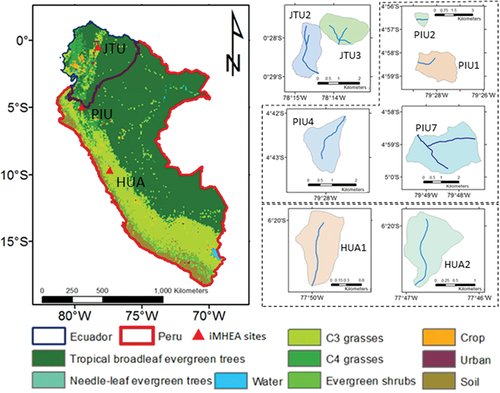
Here we explore the suitability of the simplified land cover representation described by Harper et al. (2018) to simulate typical land cover types of the upper Andean region of Perú and Ecuador, which is mainly covered by grass and shrubland vegetation on top of soils derived from volcanic materials such as Andosols, Leptosols, Histosols, Cambisols, and Regosols (FAO/IIASA/ISRIC/ISSCAS/JRC 2012, Hengl et al. 2017). The region features soils with high water retention capacity (Buytaert et al. 2005), which is found to be underestimated by the commonly used PTF parameterization (Cosby et al. 1984, Tomasella and Hodnett 1998, Hodnett and Tomasella 2002). The availability of sets of parameterizations greatly simplifies setting up JULES for large-scale applications and data-scarce regions, but it comes at the expense of a highly simplified representation and coarse classification of surface hydrological processes. Therefore, we further evaluate the effects of using modified soil data with experimental data of Andosol (Ortiz and Peralvo 2013) from site Jatunhuaycu, Ecuador (JTU; Fig. 1) for a better representation of the hydrological response of tropical Andean catchments in Piura, Perú (PIU) and Huaraz, Perú (HUA).

Figure 1. The location of the iMHEA sites within the major land cover types of the tropical Andes. JTU: Jatunhuaycu; PIU: Piura; HUA: Huaraz.

2 Materials and methods

2.1 Study region

In the tropical Andes, the major hydrological processes are defined by varying biophysical properties within various ecosystems and biomes, including páramo, jalca, puna, and montane and cloud forests (Célleri et al. 2009). The páramo, jalca, and puna are high-altitude neotropical biomes distributed over a latitudinal gradient. Approximately 35000 km² of areas in Northern Colombia and Venezuela to northern Perú are covered by páramo; jalca is found in northern to central Perú; puna can be found from central Perú to northern Argentina and Chile. Below those ecosystems, montane cloud and dry forests are characteristic vegetation types that can be found at elevations above 1000 m in the Andes, depending on the rainfall regime (Célleri et al. 2009).

The upper Andean ecosystems cover the headwaters of the major tributaries of the Amazon basin (Célleri et al. 2009) and also support smallholder irrigated agriculture, industrial consumption, and hydropower production (Buytaert et al. 2014). Despite their importance for water supply, these mountain areas are particularly vulnerable and prone to human impact. Human activities associated with rapid economic growth during the past half-century have caused drastic changes to the water cycle (Harden 2006). LUCC led by deforestation, oil exploitation, mining, and hydropower production (Zulkafli et al. 2013), and the significantly increasing demand for páramo water for intensive cattle grazing, cultivation, and pine planting (Buytaert et al. 2006), highlights the importance of water resources management.

2.2 JULES implementation

2.2.1 Model overview

JULES was originally developed by the UK Met Office as a community land surface model (Cox et al. 1999). It is commonly coupled to an atmospheric GCM or other atmospheric modelling system as the lower boundary condition (Clark et al. 2011). In addition, the stand-alone model can simulate the fluxes between the land surface and the atmosphere, which includes carbon (Clark et al. 2011), water, energy, and momentum (Best et al. 2011). It has been used successfully for various applications such as weather forecasting, climate change prediction, and earth system modelling and has been increasingly used for hydrological assessment (Zulkafli et al. 2013, Le Vine et al. 2016). JULES can be used to adequately predict the change in hydrological observations. This makes it possible to identify the potential hydrological impact under anthropogenic interventions (Rodriguez and Tomasella 2016, Boongaling et al. 2018) by changing the model structure or parameter values that represent the catchment properties. The processes of the energy exchange between various land surface and the atmosphere are simulated under the physically based approaches as described in detail by Best et al. (2011) and Clark et al. (2011).

Distinct parameters are used to calculate the energy balance for specific land use types. In this study, we reclassified the land cover types, using the survey data of Ochoa-Tocachi et al. (2018), into four vegetated plant functional types (Harper et al. 2018) – tropical broadleaf evergreen trees (BET-Tr), C3 grasses (C3), C4 grasses (C4), and evergreen shrubs (ESH) – and a non-vegetated type – bare soil (BS). We focused on the water fluxes simulated by JULES, in which precipitation is intercepted by the canopy storage, then partitioned into surface flow and infiltration into the soil based on the Hortonian infiltration excess mechanism. The saturation excess flow is calculated with a probability distributed model (PDM) described by Moore (1985), with a probability function that describes the sub-grid distribution of soil moisture (Clark and Gedney 2008). The infiltration is assumed to be redistributed instantly following the Darcy-Richards diffusion equation, which generates the subsurface flow at the lower boundaries as the gravity drainage.

2.2.2 The iMHEA catchment network

The difficulties of implementing and maintaining research-grade observation networks have historically hindered data collection in remote mountain areas, limiting the development and implementation of hydrological models to support water resources management. The advent of alternative methods for scientific data collection, particularly citizen science, provides new opportunities to alleviate data scarcity and promote public participation in hydrological science (Buytaert et al. 2014). Here, we use hydrological monitoring data from a regional citizen science-based initiative (Ochoa-Tocachi et al. 2018). The Regional Initiative for Hydrological Monitoring of Andean Ecosystems (iMHEA) aims to characterize the hydrological response of different Andean ecosystems in Perú, Ecuador, and Bolivia (Table 1). The iMHEA dataset includes streamflow, precipitation, and several weather variables at a high temporal resolution using cheap and robust technology (Buytaert et al. 2014). This monitoring is implemented in small and homogeneous catchments, distributed over the Andes between the latitudes of 0 and 17°S (Fig. 1), and covers three major high-elevation biomes: páramo, puna, and jalca (Ochoa‐Tocachi et al. 2016). Most of the catchments are rural areas covered by tussock and other grasses, wetlands, shrubs, and patches of native forest. These regions are not affected by urbanization, water abstractions, or stream alterations.

Table 1. Description of the monitored catchments. BET-Tr: tropical broadleaf evergreen trees; C3: C3 grasses; C4: C4 grasses; ESH: evergreen shrubs; BS: bare soil. The codes JTU, PIU, and HUA refer to the locations shown in Fig. 1.

Code	Ecosystem	Land use	Altitude (m)	Area (km^2)	Soil	Land cover
JTU3	Páramo	Natural	4144–4500	2.25	Andosol, Histosol	0.80 C4, 0.20 ESH
JTU2	Páramo	Grazing	4085–4322	2.42	Andosol	1.00 C4
HUA1	Humid puna	Natural	4280–4840	4.22	Andosol, Histosol	0.75 C4, 0.25 BS
HUA2	Humid puna	Grazing	4235–4725	2.38	Andosol, Histosol	0.70 C4, 0.30 BS
PIU1	Páramo	Natural	3112–3900	6.60	Andosol, Histosol	0.15 BET-Tr, 0.85 C4
PIU2	Páramo	Grazing	3245–3610	0.95	Andosol, Histosol	0.15 BS, 0.85 C4
PIU4	Forest	Natural	2682–3408	2.32	Andosol, Cambisol	0.80 BET-Tr, 0.20 C4
PIU7	Dry puna	Grazing, cultivation	3110–3660	7.80	Andosol	0.35 C3, 0.45 C4, 0.2 ESH

2.2.3 Meteorological forcing data

Precipitation was recorded in each catchment with a minimum of two tipping-bucket raingauges distributed over the catchment areas (Ochoa‐Tocachi et al. 2016), referred to here as the “iMHEA precipitation” dataset. Other meteorological data that are not available from the iMHEA network, i.e. downward shortwave and longwave radiation, temperature, specific humidity, wind speed, and surface pressure, are extracted from the Reanalysis II dataset developed by the National Centers for Environmental Prediction and the Department of Energy (NCEP-DOE; Kanamitsu et al. 2002). The dataset is available on a T62 Gaussian grid with 192 × 94 points (approximately 2° scales) and provides a six-hourly temporal resolution from January 1979 to the present. These gridded data are interpolated in space to a point scale with the nearest-neighbour interpolation method. We adjusted the NCEP-DOE temperature and pressure data from their record level to the site level using the local environmental lapse rate of 0.65°C per 100 m (Buytaert et al. 2006). For finer temporal resolution, we disaggregated the six-hourly data to hourly with linear interpolation.

2.2.4 Parameterization of high-Andean soils

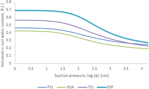
We developed the soil parameters required by JULES (Table 2) using the PTFs summarized in Table 3. The required soil composition and chemical variables are obtained from the Harmonized World Soil Database version 1.21 (FAO/IIASA/ISRIC/ISSCAS/JRC 2012) and SoilGrids (Hengl et al. 2017). The water retention properties from the local experimental data (Ortiz and Peralvo 2013) are considerably higher than those derived from PTFs (Fig. 2). Therefore, we explore using in situ experiment data from the JTU catchment (code: EXP) obtained by Ortiz and Peralvo (2013) as an alternative estimation of water retention properties for a more objective comparison. We use three sets of PTF-based and one set of experimentally based (henceforth “EXP-based”) soil properties in this study (Table 4).

Table 2. Description of soil parameters, as sourced from Best et al. (2011).

Symbol	Description	Unit
b	Exponent in soil hydraulic characteristics
φ	Saturated soil water pressure	m
Ksat	Hydraulic conductivity at saturation	kg m^−2 s^−1
θsat	Soil moisture content at saturation	m^3 m^−3
θcrit	Soil moisture content at the critical point	m^3 m^−3
θwilt	Soil moisture content at the wilting point	m^3 m^−3
hcap	Dry heat capacity	J m^−3 K^−1
hcon	Dry thermal conductivity	W m^−1 K^−1
α	Bare soil albedo

Table 3. Soil parameterization using pedotransfer functions. CL: clay fraction; SA: sand fraction; SI: silt fraction; DBD: dry bulk density (g cm⁻³); SOC: soil organic carbon (% weight); CEC: carbon exchange capacity (cmol kg⁻¹); pH: hydrogen ion activity.

Soil data	Pedotransfer function	Source
1/(n − 1)	$\mathrm{n}=\mathrm{e}\mathrm{x}\mathrm{p}\left(\left(62.986-0.833CL-0.529SOC+0.593pH+0.007C{L}^2-0.014SA\ast SI\right)/100\right)$	Hodnett and Tomasella (2002)
$1/\alpha$	$\alpha =1000\ast 9.80665/\left(1000/exp\left(\left(-2.294-3.526SI+2.440SOC-0.076CEC-11.331pH+0.019S{I}^2\right)/100\right)\right)$
Saturation point (pF = 0)	${\theta }_{sat}=0.01\left(81.799+0.099CL-31.42DBD+0.018CEC+0.451pH-0.0005SA\ast CL\right)$
Wilting point (pF = 4.2)	${\theta }_{wilt}=0.01\left(22.733-0.164SA+0.235CEC-0.831pH+0.0018C{L}^2+0.0026SA\ast CL\right)$
Critical point (pF = 2.5)	${\theta }_{crit}={\theta }_{wilt}+\frac{{\theta }_{sat}-{\theta }_{wilt}}{{\left[1+{\left(\alpha \left|\phi \right|\right)}^n\right]}^{1-1/n}}$	Van Genuchten (1980)
Saturated hydraulic conductivity	${\mathrm{K}}_{sat}=\frac{25.4}{3600}\ast {10}^{\left(-0.60-0.0064CL+0.0126SA\right)}$	Cosby et al. (1984)
Saturated heat conductivity	$\mathrm{h}\mathrm{c}\mathrm{o}\mathrm{n}={\lambda }_{air}^{\theta \mathrm{s}\mathrm{a}\mathrm{t}}{\left({\lambda }_c^{Fc}{\lambda }_s^{Fs}{\lambda }_{si}^{Fsi}\right)}^{1-\theta \mathrm{s}\mathrm{a}\mathrm{t}}$$\lambda \text{s}=\lambda \text{si}=1.57025W{m}^{\text{-1}}{K}^{\text{-1}};\lambda \text{c}=1.16025W{m}^{-1}{K}^{-1}$; $\lambda \text{air}=0.025W{m}^{-1}{K}^{-1}$	Dharssi et al. (2009)
Heat capacity	$\text{Cs}=\text{Csi}=2.133\text{*}{10}^{6}0.7exJ{m}^{-3}{K}^{-1};\text{Cc}=2.373\text{*}{10}^{6}0.7exJ{m}^{-3}{K}^{-1}$

Table 4. Soil parameters used in this study’s JULES set-up.

Catchment	n	α	θsat	θcrit	θwilt	hcon	hcap	K
PTF-based
PIU	1.359	2.288	0.463	0.333	0.217	0.219	1 189 944	0.0034
HUA	1.386	2.364	0.422	0.280	0.167	0.264	1 259 371	0.0066
JTU	1.319	1.715	0.565	0.387	0.161	0.149	938 753	0.0052
EXP-based
EXP	1.446	0.850	0.689	0.497	0.221	0.090	668 588	0.0051

Figure 2. Water retention curves obtained from PTF estimation (PIU, HUA, JTU) and in situ investigations in the JTU catchment (EXP)2013.

2.2.5 Routing

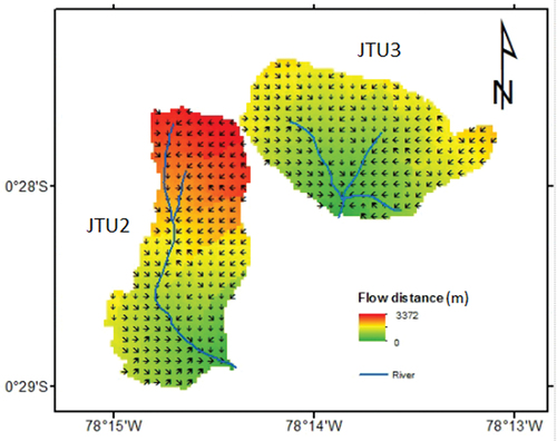
We simulate surface (Q_surface) and subsurface (Q_subsurface) runoff fluxes in distributed mode with a defined grid (30-m resolution). For a reasonable comparison to the observed river flows (Best et al. 2011), we applied a simple delay function to account for the routing delay in the river discharge (Q_sim) in each time step (t).

(1) $\begin{array}{rl}& {\mathrm{Q}}_{sim,t}=\sum _{i=1}^n\left(Q_{surface,t-t_{i1}}+Q_{subsurface,t-t_{i2}}\right);t_{i1}=\frac{d_i}{C_{surface}};\\ & t_{i2}=\frac{d_i}{C_{subsurface}}\hspace{0.17em}\end{array}$(1)

We calculate the distance (d) of each point (i) in the catchment to the outlet using the D8 flow routine (Fig. 3) with the Digital Elevation Model (DEM) obtained from Ochoa-Tocachi et al. (2018). The lag time was obtained empirically by analysing the time interval between the maximum rainfall and the peak discharge of the observed hydrograph.

Figure 3. D8 flow routine in the catchment: (a) JTU2; (b) JTU3.

2.2.6 Model evaluation

The water balance was assessed by the rainfall–runoff ratio (RR) between the total flow (Q) and the total rainfall volume (P) over the monitored period, which gives a direct indication of the water yield.

(2) $\begin{array}{c}\mathrm{R}\mathrm{R}=\frac{Q}{P}\end{array}$(2)

The baseflow sustaining the ecosystem between rainfall events was assessed using the baseflow index (BFI) and an indicator based on the slope of the flow duration curve (R2FDC). BFI defines the ratio of baseflow (Q_base) to the total flow. For dry weather runoff assessment, the baseflow was separated from the total flow using the two-parameter algorithm of Chapman (1999).

(3) $\begin{array}{c}\mathrm{B}\mathrm{F}\mathrm{I}=\frac{Q_{base}}{Q}\end{array}$(3)

R2FDC is defined as the slope in the middle third (between Q₆₆ and Q₃₃) of the flow duration curve on a logarithmic y-axis, which was used to assess the long-term hydrological regulation capacity (Olden and Poff 2003). A lower slope (near 0) indicates a higher hydrological regulation capacity:

(4) $\begin{array}{c}\mathrm{R}2\mathrm{F}\mathrm{D}\mathrm{C}=\frac{{log}_{10}{Q}_{66}-{log}_{10}{Q}_{33}}{0.66-0.33}\end{array}$(4)

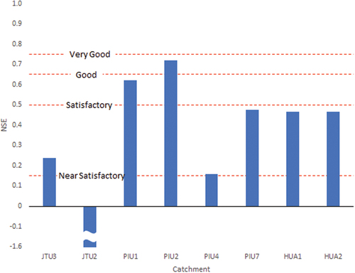
We evaluated the overall model performance using the Nash-Sutcliffe efficiency (NSE) (Nash and Sutcliffe 1970), where Q_obs,mean is the mean of observed flow, and Q_obs,t and Q_mod,t are the observed flow and modelled flow, respectively, at time step t. NSE can range from −∞ to 1. For monthly flow evaluation, a score between 1 and 0.75 is marked as “very good”; between 0.75 and 0.65 is marked as “good,” and between 0.65 and 0.5 is marked as “satisfactory” (Moriasi et al. 2007). NSE scores lower than 0.5 are marked as “unsatisfactory.” However, for modelling based on daily flow, the NSE tends to be lower because of the high flow variability at that time step, so we label NSE values in the range of 0.15 to 0.5 as “near satisfactory,” in line with other studies (Dos Santos et al. 2020).

(5) $\begin{array}{c}\mathrm{N}\mathrm{S}\mathrm{E}=1-\frac{{\sum }_t^N{\left(Q_{mod,t}-Q_{obs,t}\right)}^2}{{\sum }_t^N{\left(Q_{obs,t}-Q_{obs,mean}\right)}^2}\end{array}$(5)

3 Results

Here we investigate the adequacy of the JULES modelling using PTF-based and EXP-based soil parameter sets, compared to the observed flow in the investigated catchments (Figs 4 and Figs 5a).

Figure 4. Left: a comparison of the observed and modelled flows of (a) JTU3, (b) JTU2, (c) HUA1, and (d) HUA2. Right: flow duration curves of the same hydrographs.

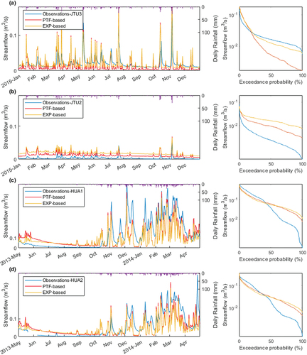
Figure 5. Left: a comparison of the observed and modelled flows of (a) PIU1, (b) PIU2, (c) PIU4, and (d) PIU7. Right: flow duration curves of the same hydrographs.

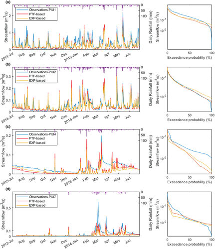
Figure 6. NSE score of the modelling flow in each catchment.

Figure 4(a) shows the hydrograph for the JTU3 catchment, which is characterized by a streamflow variation with low seasonality. The two parameter sets produce similar simulations of the peak flows. However, we find a considerable increase in baseflow when using EXP-based parameters. Peak flow events are well detected by the model, while some events are considerably overestimated (e.g. March–June 2015).

JTU2 (Fig. 4(b)) also features low seasonality. The flow is generally overestimated during the observed period in the model simulations using either PTF-based or EXP-based parameters. Most of the peak flow events are overestimated but detected under each parameter set.

Similar hydrology regimes are found in HUA1 (Fig. 4(c)) and HUA2 (Fig. 4(d)). These two catchments are both characterized by high seasonality, in which the wet season extends between November and April, followed by a long dry season. We find that the modelling with either the PTF-based or EXP-based data can provide a fairly good fit with the observation curve, in which most of the peak flows are underestimated, which is also the case for the dry season flows.

Low seasonality is found in PIU1 (Fig. 5(a)) and PIU2 (Fig. 5(b)), whereas PIU4 (Fig. 5(c)) and PIU7 (Fig. 5(d)) present high seasonality. In PIU1/PIU2, most of the peak flows and recessions are well simulated. A certain underestimation of flows is found in PIU1 during January to February 2015. In PIU2, some peak flow events are overestimated (e.g. November and December 2014). Lower baseflow is simulated by using the PTF-based parameters, which are better fitted to the observed values.

In PIU4 (Fig. 5(c)), both the PTF-based and EXP-based parameterizations underestimated the baseflow in the dry season. Certain peak flow events are overestimated (e.g. November 2015 and February 2016), while the main gap is found during the recession processes during the wet season. In PIU7 (Fig. 5(d)), the simulated flow is higher when using the PTF-based parameters. However, most of the peak flow events are detected using either parameter set. The simulated baseflow is close to the observed values in June 2014. The most significant gap is found during March 2014, where the simulated peak flow is considerably lower than the observed values.

Table 5 summarizes the performance of the JULES model driven by both the PTF-based and EXP-based soil properties. In catchment JTU3, the PTF-based parameter set simulates lower flows than the observed value (RR: 0.261 vs 0.380). The EXP-based parameter set simulates a larger total flow, which is closer to the observed value (RR: 0.325 vs 0.380). A higher percentage of baseflow is simulated under the experimental values (BFI: 0.460 vs 0.266), whilst the flow duration curve is closer to its observed value (R2FDC: −0.80 vs −0.51). The overall performance is near satisfactory under the EXP-based set-up (NSE: 0.239).

Table 5. Hydrological summary indices as calculated from the observed and modelled flow time series based on a daily time step in this study. OBS: observations; PTF: PTF-based set-up; EXP: EXP-based set-up; RR: rainfall–runoff ratio; BFI: baseflow index; R2FDC: slope of the flow duration curve; NSE: Nash-Sutcliffe efficiency. The codes JTU, PIU, and HUA refer to the locations shown in Fig. 1.

Site	Soil set	RR	BFI	R2FDC	NSE
JTU3	OBS	0.380	0.712	−0.51	n/a
	PTF	0.261	0.266	−1.78	0.057
	EXP	0.325	0.460	−0.80	0.239
JTU2	OBS	0.071	0.577	−1.03	n/a
	PTF	0.189	0.737	−0.76	−1.550
	EXP	0.294	0.858	−0.43	−5.300
HUA1	OBS	0.638	0.674	−3.23	n/a
	PTF	0.528	0.563	−1.09	0.467
	EXP	0.492	0.577	−0.86	0.435
HUA2	OBS	0.579	0.712	−2.93	n/a
	PTF	0.511	0.574	−1.20	0.467
	EXP	0.474	0.579	−0.83	0.416
PIU1	OBS	0.686	0.425	−1.29	n/a
	PTF	0.460	0.424	−1.16	0.620
	EXP	0.461	0.519	−0.91	0.589
PIU2	OBS	0.639	0.598	−1.37	n/a
	PTF	0.550	0.440	−1.33	0.719
	EXP	0.546	0.522	−1.00	0.745
PIU4	OBS	0.360	0.858	−0.99	n/a
	PTF	0.230	0.675	−1.65	0.193
	EXP	0.220	0.752	−1.02	0.160
PIU7	OBS	0.269	0.703	−1.18	n/a
	PTF	0.199	0.709	−1.05	0.474
	EXP	0.142	0.721	−0.73	0.283

For the JTU2 catchment, the PTF-based parameter set gives a better fit than the experimental parameter set. However, the observed RR is unrealistically low (0.071; Fig. 4(c)), which casts doubts on the quality of those observations. This may also be the reason for the unsatisfactory model performance under both set-ups (NSE: −1.55/−5.30).

In the conserved puna catchment HUA1, both set-ups underestimate the average flow (RR: 0.528/0.492 vs 0.638). The simulated flow duration curve is consequently steeper (Fig. 4(c); R2FDC: −1.09/−0.86 vs −3.23). A lower ratio of baseflow (BFI: 0.563/0.577 vs 0.674) is simulated compared to the observed values. However, the overall model performances are near satisfactory under both set-ups (NSE: 0.467/0.435). Similar results are found in the grazed puna catchment HUA2.

In PIU1, the JULES run driven by the parameter values estimated using the PTF-based parameters underestimates the runoff by 32.9% (RR: 0.460 vs 0.686) but has a baseflow ratio (BFI: 0.424 vs 0.425) and regulation capacity (R2FDC: −1.16 vs −1.29) similar to the observations. For the experimental values, there is barely a difference in the overall flow (RR: 0.461), whereas a higher percentage of baseflow (BFI: 0.519) and flatter flow duration curve (R2FDC: −0.91) are simulated. The model performance is satisfactory under both set-ups (NSE: 0.620 vs 0.589).

In the adjacent catchment PIU2, the parameters estimated with the PTF-based parameterization yield a lower runoff than the observed value (RR: 0.550 vs 0.639), whereas the slope of the flow duration curve is closer to the observed value (R2FDC: −1.33 vs −1.37). A higher baseflow ratio is simulated under the experimental parameter set-up (BFI: 0.522) with a minor change in the total water yield. The overall model performance is good for both set-ups (NSE: 0.719/0.745).

In PIU4, both set-ups underestimate the total flow (RR: 0.230/0.220) compared to its observed value (RR: 0.360). The modelling flows are underestimated under all flow regimes, characterized by their lower baseflow estimation (BFI: 0.675/0.752). A modelling performance of a near satisfactory level is found under both set-ups (NSE: 0.193/0.160).

In PIU7, the average flow is considerably lower than the observed value for both set-ups (RR: 0.199/0.142 vs 0.269). The gap mainly exists in the peak flow, whilst the percentage of baseflow is close to observed values (BFI: 0.709/0.721 vs 0.703). For the PTF-based parameters, the middle third of the flow duration curve is closer to the observations (R2FDC: −1.05 vs −1.18). A near satisfactory performance is simulated under the PTF-based set-up (NSE: 0.474 vs 0.283).

We evaluated the difference in model performance between standard PTF parameter sets and the experimental parameter sets obtained from representative soils. The latter simulates higher model performance in two out of eight catchments (JTU3 and PIU4), whilst the PTF-based parameters show better performance in the rest of the catchments. Using the most suitable set-up in each case, seven out of eight catchments are marked as at least “near satisfactory” (Fig. 6).

4 Discussion

4.1 Simulated hydrographs

The results of this study show that the simulation of streamflow phenomena in each catchment based on the JULES model, by both EXP-based and PTF-based parameterizations, produces a generally good agreement between the simulated value and the observed value in low-seasonality catchments (Fig. 5(a), PIU1; Fig. 5(b), PIU2). For high-seasonality catchments, simulations often underestimate the actual flow rate during dry periods (Fig. 5(c), PIU4). The upper Andean region of Perú and Ecuador is mainly covered by the Andean páramo (Buytaert et al. 2006) biome. Volcanic soils are the dominant soil types, among which Andosols are particularly common (FAO/IIASA/ISRIC/ISSCAS/JRC 2012). These types of soils cover the páramo ecosystem in large parts of the tropical Andean mountain belt (Buytaert et al. 2005), which provides key hydrological services in montane environments. These soils are dark, humic and acidic with an open pore structure, in which organic matter and volcanic ash accumulate (Crespo et al. 2011). Thus, Andosols are known for their extremely high water retention capacity (0.64–0.93m³m^–3 at saturation) (Buytaert 2004) with high organic carbon content (13–36%) and low bulk density (0.2–0.8 g cm^–3). These properties of soil structure may have an important effect on the hydrological regime.

A detailed characterization of soil properties was conducted to understand the subsurface water transport and tracer mixing in these Andosols at three locations along a steep hillslope in the upper Andean region (Mosquera et al. 2020). The soil moisture observations in the horizon showed a fast-responding (few hours) “rooted” layer to a depth of 15 cm, overlying a “perched” layer (52–61 cm depth) that remained near saturated year-round. Isotopic signatures revealed that water resides within this soil horizon for short periods, in both the rooted (two weeks) and the perched (four weeks) layer. The behaviour resembles that of a “layered sponge” in which vertical flowpaths are dominant. That is, on the one hand, a perched water layer forms that maintains high-moisture near-saturated conditions year-round due to the presence of a low conductivity layer below a layer with a higher conductivity. On the other hand, there is fast vertical transport of water due to the rapid transfer of hydraulic potentials along the entire soil profile, facilitating water mobilization through the porous soil matrix. Despite the dominance of vertical flowpaths, lateral flow likely develops during high-intensity rainstorm events above hydraulically restrictive layers (e.g. the perched layer) due to the steep hillslope.

The large water storage capacity of these soils, which is often referred to as a “sponge-like” structure, may have a major impact on the observed hydrographs, which the model may still struggle to represent adequately. As shown in Fig. 4(a) (JTU3 catchment), the “EXP-based” parameterization overestimates virtually all peaks, while it underestimates the flow the rest of the time. The effects of this sponge-like behaviour vary with climate, especially the rainfall rate and the seasonality. As rainfall increases, and with lower seasonality, the impact of the sponge effect becomes negligible. This phenomenon can be clearly seen from the hydrographs in Fig. 5(a), in which the PIU1 catchment has uniformly distributed rainfall. In this case, the theoretical simulation and the observed hydrographs coincide very well.

4.2 Modelling performance

Overall, our JULES model set-up shows that it is possible to simulate the streamflow of the dominant land cover types of the upper tropical Andes. Modelling results from two out of eight catchments are marked as “satisfactory” under a baseline used to assess monthly flow (Moriasi et al. 2007). For our simulation based on a daily time scale, seven out of eight catchments are at least “near satisfactory” under an acceptable standard (Coffey et al. 2004, Nejadhashemi et al. 2012, Dos Santos et al. 2020). The main outlier is the JTU2 catchment, where the simulated flows are considerably higher than the observed values. One possible explanation is that this catchment has an unrealistically low observed water yield for this biome (RR: 0.071). This observation suggests that subsurface and groundwater preferential flow pathways exist in the deep soil layers, bypassing the flow gauging station and introducing an error that led to an underestimation of the catchment water balance (Buytaert et al. 2006, Ochoa‐Tocachi et al. 2016).

In JTU3, we observe a modest improvement in model performance when the standard PTF parameter sets are replaced with experimental parameter sets. The main improvements are observed in the BFI and the slope of the flow duration curve, representing the partitioning of the rainfall in surface and subsurface response. In PIU4, the NSE score is slightly lower using the experimental parameter sets. There is a relatively small difference in the average flow between the two parameter sets. However, the baseflow ratio and the slope of the flow duration curve are much closer to the observed values with the EXP-based simulation. Therefore, we suggest this parameter set be used in the catchment. For these two catchments, the simulation using EXP-based parameters has improved the baseflow estimation considerably. However, it still presents a lower level of baseflows than the catchments actually generated. This is commonly attributed to the occurrence of hydrologically disconnected wetlands, which store water and release it gradually during dry periods (Buytaert and Beven 2011), as similar modelling results are also found in the lower Andean basins (Zulkafli et al. 2013).

For the other five catchments (except JTU2), the PTF-based parameter set gives a better estimation for the hydrological regime. We find that the PTF-based parameter sets generate a lower fraction of baseflow than the experimental parameter sets, which is also lower than the observed values in these catchments. One possible explanation is the overestimation of evaporation by JULES, which was also highlighted by Martínez-de la Torre et al. (2019). A possible solution is to reduce evapotranspiration by lowering soil moisture availability (Blyth et al. 2019). We compare the effects on hydro-physical soil properties between two sets of water retention properties. The PTF underestimates the values of saturated water content (i.e. 0.689 vs 0.565 in JTU) and residual water content (i.e. 0.221 vs 0.161 in JTU) compared to the values obtained from local experiments. This is not a surprise, given the exceptionally large water retention capacities of many high-Andean soils. The experimental data result in only a very slight increase in soil water storage capacity. However, these parameters have resulted in a higher soil moisture availability factor (β_k; see Best et al. 2011), which suppresses the lower vegetation transpiration rates. This may explain the higher runoff ratios observed in the experimental parameter set runs.

In addition to the difficulty of smaller time-scale hydrological modelling, the gap between the modelling and the observations can be attributed to several remaining sources of uncertainty. First, the meteorological input data are prone to uncertainty. The spatiotemporal rainfall variability in high-mountain areas such as the Andes is extremely high, complicating the extrapolation of point-based measurements to catchment averages. The insufficient representative rainfall can lower the model performance in these tropical catchments (Zulkafli et al. 2013), as micro-climates might occur within a scale of 4 km (Buytaert et al. 2006). In our study, we find that peak flows can be over/underestimated due to the potentially over/underestimated rainfall (e.g. overestimated in PIU2: December 2015, PIU4: November 2015; and underestimated in PIU7: March 2014).

Next, the representativeness of the observed soil characteristics can be questioned. As for the rainfall measurements, issues of incommensurability remain because of the difference in scale between the soil samples and catchment-averaged soil properties required by the model. The lack of in situ soil data for most catchments also required us to use the data from a single catchment in Ecuador for all sites. The transfer parameters could reasonably simulate the hydrology, assuming that the catchments have similar water retention properties (Heuvelmans et al. 2004). Our results show that the data are representative of the ecosystems hosted by the catchments; this extrapolation can introduce substantial errors.

Despite these shortcomings, our results show that it is possible to develop soil parameter sets for large-scale, physics-based hydrological models, which improve upon the default parameter sets yet are sufficiently representative for a land surface class to be applied at a regional scale. The expanding configurations enable models such as JULES to be implemented for data-scarce regions where local in situ data are not available.

5 Conclusions

We implement the hydrological model JULES in eight tropical Andean catchments to evaluate the performance of the commonly used parameter values and regionally representative experimentally derived soil parameters. We find that the conventional JULES set-up can represent key hydrological fluxes. However, the surface–subsurface partitioning is especially problematic, while this approach also overestimates vegetation transpiration. These processes are sensitive to the soil water retention parameters (saturated, critical, and wilting point). The soil moisture extraction of high-Andean soils can be suppressed by using the water retention curve from experimental soil data. We find that these experimentally based parameter values have altered both the flow partitioning and catchment water balance in the simulations. In particular, the parameters improve baseflow simulation, which is more suitable for use in some baseflow-dominated catchments. However, the improvements indicate that several other sources of uncertainty remain, mainly arising from the input data and subsurface flow residence times. In addition, the experimental data we extrapolated from one sample is not representative enough for all study catchments. Nevertheless, our results suggest that the hydro-physical soil properties greatly affect the hydrological regime, especially in terms of the surface–subsurface partitioning. It is important to further investigate these effects as well as to develop regional parameter sets for different soil types that complement the existing land cover datasets that come with JULES.

Acknowledgements

The authors gratefully acknowledge the people and authorities of Andean communities who have provided essential and constant consent and support to our fieldwork. We thank all partners of the Regional Initiative for Hydrological Monitoring of Andean Ecosystems (iMHEA), mainly FONAG, Nature and Culture International (NCI), APECO, The Mountain Institute, and CONDESAN, who provided the data presented here. All iMHEA partners funded fieldwork. In addition, we acknowledge the important contributions of Charles Zogheib (Imperial College), Bert De Bièvre, Paola Fuentes and Enrique (FONAG).

Disclosure statement

No potential conflict of interest was reported by the authors.

Additional information

Funding

This work was supported by Natural Environment Research Council: NE/K010239/1 and NE/I004017/1. HKC was funded by Taiwan Top University Strategic Alliance PhD Scholarships – Imperial PhD Scholarships of the Ministry of Education, Taiwan. BOT was funded by an Imperial College President’s PhD Scholarship and the “Science and Solutions for a Changing Planet” DTP (NERC grant NE/L002515/1) and acknowledges the National Secretariat of Higher Education, Technology, and Innovation of Ecuador (SENESYCT).

References

- Best, M.J., et al., 2011. The joint UK land environment simulator (JULES), model description–Part 1: energy and water fluxes. Geoscientific Model Development, 4 (3), 677–699. doi:10.5194/gmd-4-677-2011
- Blyth, E.M., Martinez-de la Torre, A., and Robinson, E.L., 2019. Trends in evapotranspiration and its drivers in Great Britain: 1961 to 2015. Progress in Physical Geography: Earth and Environment, 43 (5), 666–693. doi:10.1177/0309133319841891
- Boongaling, C.G.K., Faustino-Eslava, D.V., and Lansigan, F.P., 2018. Modeling land use change impacts on hydrology and the use of landscape metrics as tools for watershed management: the case of an ungauged catchment in the Philippines. Land Use Policy, 72, 116–128. doi:10.1016/j.landusepol.2017.12.042
- Buytaert, W., 2004. The properties of the soils of the south Ecuadorian páramo and the impact of land use changes on their hydrology. Doctoral dissertation. Katholieke Universiteit Leuven.
- Buytaert, W., et al., 2005. The effect of land‐use changes on the hydrological behaviour of Histic Andosols in south Ecuador. Hydrological Processes: An International Journal, 19 (20), 3985–3997. doi:10.1002/hyp.5867
- Buytaert, W., et al., 2006. Human impact on the hydrology of the Andean páramos. Earth-Science Reviews, 79 (1–2), 53–72. doi:10.1016/j.earscirev.2006.06.002
- Buytaert, W. and Beven, K., 2011. Models as multiple working hypotheses: hydrological simulation of tropical alpine wetlands. Hydrological Processes, 25 (11), 1784–1799. doi:10.1002/hyp.7936
- Buytaert, W., et al., 2014. Citizen science in hydrology and water resources: opportunities for knowledge generation, ecosystem service management, and sustainable development. Frontiers in Earth Science, 2, 26. doi:10.3389/feart.2014.00026.
- Célleri, R. and Feyen, J., 2009. The hydrology of tropical Andean ecosystems: importance, knowledge status, and perspectives. Mountain Research and Development, 29 (4), 350–356. doi:10.1659/mrd.00007
- Célleri, R., et al., 2009. Understanding the hydrology of tropical Andean ecosystems through an Andean Network of Basins. IAHS-AISH Publication, 336, 209–212.
- Chapman, T., 1999. A comparison of algorithms for stream flow recession and baseflow separation. Hydrological Processes, 13 (5), 701–714. doi:10.1002/(SICI)1099-1085(19990415)13:5<701::AID-HYP774>3.0.CO;2-2
- Clark, D.B. and Gedney, N., 2008. Representing the effects of subgrid variability of soil moisture on runoff generation in a land surface model. Journal of Geophysical Research: Atmospheres, 113 (D10). doi:10.1029/2007JD008940
- Clark, D.B., et al., 2011. The Joint UK Land Environment Simulator (JULES), model description–Part 2: carbon fluxes and vegetation dynamics. Geoscientific Model Development, 4 (3), 701–722. doi:10.5194/gmd-4-701-2011
- Coffey, M.E., et al., 2004. Statistical procedures for evaluating daily and monthly hydrologic model predictions. Transactions of the ASAE, 47 (1), 59. doi:10.13031/2013.15870
- Cosby, B.J., et al., 1984. A statistical exploration of the relationships of soil moisture characteristics to the physical properties of soils. Water Resources Research, 20 (6), 682–690. doi:10.1029/WR020i006p00682
- Cox, P.M., et al., 1999. The impact of new land surface physics on the GCM simulation of climate and climate sensitivity. Climate Dynamics, 15 (3), 183–203. doi:10.1007/s003820050276
- Crespo, P.J., et al., 2011. Identifying controls of the rainfall–runoff response of small catchments in the tropical Andes (Ecuador). Journal of Hydrology, 407 (1–4), 164–174. doi:10.1016/j.jhydrol.2011.07.021
- Dharssi, I. et al., 2009. New soil physical properties implemented in the Unified Model at PS18, Met Office Technical Report 528.
- Dos Santos, F.M., de Oliveira, R.P., and Mauad, F.F., 2020. Evaluating a parsimonious watershed model versus SWAT to estimate streamflow, soil loss and river contamination in two case studies in Tietê river basin, São Paulo, Brazil. Journal of Hydrology: Regional Studies, 29, 100685.
- FAO/IIASA/ISRIC/ISSCAS/JRC, 2012. Harmonized world soil database (version 1.2). FAO, Rome, Italy.
- Harden, C.P., 2006. Human impacts on headwater fluvial systems in the northern and central Andes. Geomorphology, 79 (3–4), 249–263. doi:10.1016/j.geomorph.2006.06.021
- Harper, A.B., et al., 2018. Vegetation distribution and terrestrial carbon cycle in a carbon cycle configuration of JULES4. 6 with new plant functional types. Geoscientific Model Development, 11 (7), 2857–2873. doi:10.5194/gmd-11-2857-2018
- Hengl, T., et al., 2017. SoilGrids250m: global gridded soil information based on machine learning. PLoS One, 12 (2), e0169748. doi:10.1371/journal.pone.0169748
- Heuvelmans, G., Muys, B., and Feyen, J., 2004. Evaluation of hydrological model parameter transferability for simulating the impact of land use on catchment hydrology. Physics and Chemistry of the Earth, Parts a/B/C, 29 (11–12), 739–747. doi:10.1016/j.pce.2004.05.002
- Hodnett, M.G. and Tomasella, J., 2002. Marked differences between van Genuchten soil water-retention parameters for temperate and tropical soils: a new water-retention pedo-transfer functions developed for tropical soils. Geoderma, 108 (3–4), 155–180. doi:10.1016/S0016-7061(02)00105-2
- Kanamitsu, M., et al., 2002. NCEP–DOE AMIP-II Reanalysis (R-2). Bulletin of the American Meteorological Society, 83 (11), 1631–1643. doi:10.1175/BAMS-83-11-1631(2002)0832.3.CO;2
- Le Vine, N., et al., 2016. Diagnosing hydrological limitations of a land surface model: application of JULES to a deep-groundwater chalk basin. Hydrology and Earth System Sciences, 20 (1), 143–159. doi:10.5194/hess-20-143-2016
- Marthews, T.R., et al., 2014. High-resolution hydraulic parameter maps for surface soils in tropical South America. Geoscientific Model Development, 7 (3), 711–723. doi:10.5194/gmd-7-711-2014
- Martínez-de la Torre, A., Blyth, E.M., and Weedon, G.P., 2019. Using observed river flow data to improve the hydrological functioning of the JULES land surface model (vn4. 3) used for regional coupled modelling in Great Britain (UKC2). Geoscientific Model Development, 12 (2), 765–784. doi:10.5194/gmd-12-765-2019
- McIntyre, N., et al., 2014. Modelling the hydrological impacts of rural land use change. Hydrology Research, 45 (6), 737–754. doi:10.2166/nh.2013.145
- Moore, R.J., 1985. The probability-distributed principle and runoff production at point and basin scales. Hydrological Sciences Journal, 30 (2), 273–297. doi:10.1080/02626668509490989
- Moriasi, D.N., et al., 2007. Model evaluation guidelines for systematic quantification of accuracy in watershed simulations. Transactions of the ASABE, 50 (3), 885–900. doi:10.13031/2013.23153
- Mosquera, G.M., et al., 2020. Water transport and tracer mixing in volcanic ash soils at a tropical hillslope: a wet layered sloping sponge. Hydrological Processes, 34 (9), 2032–2047. doi:10.1002/hyp.13733
- Nash, J.E. and Sutcliffe, J.V., 1970. River flow forecasting through conceptual models part I—A discussion of principles. Journal of Hydrology, 10 (3), 282–290. doi:10.1016/0022-1694(70)90255-6
- Nejadhashemi, A.P., Wardynski, B.J., and Munoz, J.D., 2012. Large-scale hydrologic modeling of the Michigan and Wisconsin agricultural regions to study impacts of land use changes. Transactions of the ASABE, 55 (3), 821–838. doi:10.13031/2013.41517
- Ochoa-Tocachi, B.F., et al., 2018. High-resolution hydrometeorological data from a network of headwater catchments in the tropical Andes. Scientific Data, 5, 180080. doi:10.1038/sdata.2018.80
- Ochoa‐Tocachi, B.F., et al., 2016. Impacts of land use on the hydrological response of tropical Andean catchments. Hydrological Processes, 30 (22), 4074–4089.
- Olden, J.D. and Poff, N.L., 2003. Redundancy and the choice of hydrologic indices for characterizing streamflow regimes. River Research and Applications, 19 (2), 101–121. doi:10.1002/rra.700
- Ortiz, E. and Peralvo, M., 2013. Restauración de áreas degradadas de páramo a pequeña escala y diseño de un plan piloto de manejo adaptativo para zonas de amortiguamiento dentro de las microcuencas Antisana y Pita en áreas de aporte a los sistemas de agua potable del Distrito Metropolitano de Quito. Quito: CONDESAN.
- Rodriguez, D.A. and Tomasella, J., 2016. On the ability of large-scale hydrological models to simulate land use and land cover change impacts in Amazonian basins. Hydrological Sciences Journal, 61 (10), 1831–1846.
- Tomasella, J. and Hodnett, M.G., 1998. Estimating soil water retention characteristics from limited data in Brazilian Amazonia. Soil Science, 163 (3), 190–202. doi:10.1097/00010694-199803000-00003
- Tsarouchi, G. and Buytaert, W., 2018. Land-use change may exacerbate climate change impactson water resources in the Ganges basin. Hydrology and Earth System Sciences, 22 (2), 1411–1435. doi:10.5194/hess-22-1411-2018
- Turner, B.L., Meyer, W.B., and Skole, D.L., 1994. Global land-use/land-cover change: towards an integrated study. Ambio.Stockholm, 23 (1), 91–95.
- Van Genuchten, M.T., 1980. A closed‐form equation for predicting the hydraulic conductivity of unsaturated soils. Soil Science Society of America Journal, 44 (5), 892–898. doi:10.2136/sssaj1980.03615995004400050002x.
- Zulkafli, Z., et al., 2013. A critical assessment of the JULES land surface model hydrology for humid tropical environments. Hydrology and Earth System Sciences, 17 (3), 1113–1132. doi:10.5194/hess-17-1113-2013