Identifying potential systemic changes in a regulated river: a diagnostic methodology based on whiteness property of innovation sequences

ABSTRACT

Traditional hydrological routing schemes are structured in reference to a pre-assumed time-invariant inflow–storage–outflow function. In light of this, potential systemic changes arising from river regulation cannot be accommodated in such a static model structure. As such, a diagnostic methodology is developed in this study to examine the presence of potential systemic changes and recognize time spans in which the adopted inflow–storage–outflow function is inadequate to represent the functional behaviour of the system. This is done objectively by developing a two-step change-point detection algorithm based on the whiteness property of the innovation sequence. Using four carefully designed numerical experiments, our findings reveal that the proposed methodology (a) objectively detects the non-stationary behaviour in streamflow time series associated with systemic changes, (b) properly tracks the pathway of structural evolution of a hydrological routing model, and (c) automatically identifies time periods wherein a river routing model structure needs to be updated.

KEYWORDS:

• systemic change
• flow regime alteration
• model structure inadequacy
• innovation whiteness property
• change-point detection

Editor A. Fiori

Associate Editor V. Samadi

1 Introduction

A typical problem in operational hydrology is to simulate the rainfall–runoff process emerging from a drainage basin and then route the resulting streamflow hydrograph through the river corridor. Such prediction plays a significant role in the analysis and design of various hydraulic structures including flood protection structures, flood warning systems, and river training works. Three basic procedures – the hydrological, hydraulic, and black-box modelling approaches – are currently in use to route the streamflow hydrograph through the river corridor (Hasanvand et al. 2013). Among the three cited approaches, the hydrological routing approach has a simpler structure and data requirements compared to the latter two procedures. However, ironically, it is assumed that the inflow–storage–outflow function of a typical hydrological model has a certain and invariant mathematical structure throughout the simulation period and along the river course (Kim and Georgakakos 2014). This assumption is questionable because it ignores potential systemic changes in the relationship caused by natural processes and/or anthropogenic activities. Here, a typical systemic change is defined as a significant change in the structure and/or behaviour of the system under consideration (Polhill et al. 2016). From a modelling standpoint, this means that a certain transition rule in model structure and/or its parameters, for which they were previously acceptable, need to be adapted at a certain point in time so that it can continue to properly capture the dynamics of system behaviour (Verstegen et al. 2016).

Generally speaking, the natural flow regime of rivers and streams is being altered significantly by dams, flood-control projects, and other human activities (Slater et al. 2021). Among these, dams, as the most prevalent cause of river flow regime alteration, are one of the main factors in controlling the ecological integrity and physical properties of river channels (Graf 2006, Zuo et al. 2019). Theoretically, altering the hydrological regime of a natural channel through its regulation, upstream watershed land use, and climate change can lead to physical responses along its corridor (Poff et al. 1997, Mathews and Richter 2007, Buechel et al. 2022). For a given reach, by changing the size of streambed substrate, river morphology, and inundation areas, physical readjustments to a disturbance event can bring about systemic change and consequently affect flood wave propagation within the river corridor (Hall et al. 2014, Slater et al. 2015, Feng et al. 2019). However, due to the progressive nature of change in a natural channel, systemic change is expected to be gradual. Besides, the pathway of response is considered to be highly fluctuating and poorly understood due to being affected by many factors including the inherent resistance, the available energy, the river system’s spatial extent, and the severity of the disturbance event (Poeppl et al. 2017). In light of this, if a fluvial system experiences an intervention, to justify the logical application of a routing model, it is crucial to be able to determine whether its structure is adequate to emulate the functional behaviour of the system under post-disruption conditions or not.

Leaving aside the mass balance equation, which is applicable at various spatial and temporal scales, the structural adequacy of a typical hydrological routing model is highly related to the selection of an appropriate inflow–storage–outflow function (Singh and Scarlatos 1987, Vatankhah 2021). Accordingly, to address the research gap cited in the previous paragraph, a diagnostic method is called for to appropriately recognize the time periods of model execution during which the inflow–storage–outflow function is inadequate to represent the system behaviour. For this purpose, one possible strategy is to capitalize on information from internal diagnostics obtained by the data assimilation (DA) framework (Gustafsson 2000, Simon 2006, Reichle et al. 2008). One of the most common diagnostic procedures that has been used in the hydrological literature is to analyse the statistical properties of the innovation sequences (Rajaram and Georgakakos 1989, Georgakakos et al. 1990, Butts et al. 2004, Bennett et al. 2013, Vrugt and Sadegh 2013).

This diagnostic approach is based on the assumption that if the assumed state-space model has the correct structure and parameters, its innovations sequence will be a zero-mean white stochastic process with a known covariance matrix (Gustafsson 2000, Simon 2006). From the sequential DA perspective, innovation is defined as a one-step ahead predicted residual, and can be interpreted as a part of a measurement that holds new information (Meditch 1969). Despite the strong theoretical background behind this approach, the main drawback that can be attributed to these research activities is to assess and evaluate innovations in a subjective manner. As an example, Rajaram and Georgakakos (1989) based their assessment on a subjective measure to delineate the locations of structural inadequacy. They argue that high values of normalized innovations correspond to drastic changes in discharge measurements which could be considered points of potential structural inadequacy. However, any fluctuation of the innovations sequence does not necessarily indicate a structural inadequacy in the model, and there is a need to define objective criteria to investigate the impact of such anomalies.

Change-point analysis methods can be considered to solve this problem objectively by exploring an innovation sequence and detecting times wherein some of its statistical properties (e.g. mean, standard deviation, etc.) could change abruptly (Killick et al. 2012). The successful application of change-point analysis, whether parametric or non-parametric, to identify the number and location of change points in the statistical properties of a time series has been reported in several scientific fields (Matteson and James 2014, Sharma et al. 2016, Ciria et al. 2019, Zhou et al. 2019). However, the implementation of these change-point analysis methods has yet to be considered in diagnosing the pathway of structural evolution of a hydrological model.

In this study, the possibility of detecting the pathway of structural evolution of a hydrological routing model as a result of river regulation is investigated. For this purpose, an objective change-point detection algorithm is proposed, which basically consists of two main blocks: an innovation generator and a change-point detector. In this regard, a dual state–parameter updating kernel, within the Kalman filter (KF) framework (Kalman 1960), is coupled with the linear Muskingum model (LMM) to generate the normalized innovations sequence (McCarthy 1938). As for detecting the change points, a parametric approach based on minimizing a penalized contrast function is used to detect change points objectively. The robustness of the proposed method is evaluated through multiple scenarios based on synthetic data. The goal is to examine the ability of the proposed algorithm to detect times when the model structure loses its adequacy under post-disturbance conditions.

2 Materials and methods

2.1 The proposed methodology

As a general rule, upon confronting a dramatic change in the flow regime of a river, a typical static model structure could comply with data variability up to a certain limit, beyond which the goodness of fit will deteriorate. A basic question in this context is to explore time spans in which updating the model structure could prevent the deterioration of the measure of goodness of fit. As a result, to establish a modelling framework that better captures the dynamic behaviour of the system under consideration, it is necessary to detect systemic changes in a flood routing model structure and pursue how it will evolve over time. For this purpose, a diagnostic methodology is required to objectively delineate the number and location of change points. As such, a two-step change-detection algorithm is proposed, therefore the major contribution of this study is to generate a sequence of normalized innovation via an appropriate filter in the first step and then introduce this sequence as input to the change detector in the second step.

From a statistical change detection point of view, any state estimator (i.e. an updating kernel, also called a whitening filter) within the DA framework can receive the forcing data and available observed output, and then estimate the innovation mean and covariance matrix using statistical methods (Gustafsson 2000). Accordingly, as shown in Fig. 1, the first step in the proposed algorithm is to generate a sequence of normalized innovations to be computed via the following relation:

(1) ${\xi }_t=f\left({\upsilon }_t,S_t\right)={S_t}^{-1/2}{\upsilon }_t,t=1:n$(1)

Figure 1. Schematic representation of systematic change detection in a routing model structure.

where ${\upsilon }_t$ and $S_t$ are the innovation and its variance-covariance matrix at an instant in time, respectively, which will be further discussed in Section 2.2.

Assuming an ideal model structure, a typical DA framework that estimates states and parameters of the system simultaneously results in uncorrelated successive innovations due to its potential to explicitly address different sources of uncertainties arising from initial conditions, observations, and parameters. Indeed, it has been assumed that if errors associated with the cited sources of uncertainty are being addressed properly, potential detected changes in the normalized innovations sequence could be related to uncertainties due to model structure. Traditionally, either of the following methods could be adopted to simultaneously estimate the states and parameters within a DA framework at each time step: (1) state augmentation, where the state vector is extended by adding parameter variables so that estimation of model states and parameters happens concurrently (Hendricks Franssen and Kinzelbach 2008, Smith et al. 2013); or (2) dual state–parameter estimation, where parameters and states are estimated separately through two successive filters (Moradkhani et al. 2005, Leisenring and Moradkhani 2012). The main difference between the two approaches arises from their updating step, where – unlike in the augmented approach – systematic errors in the predictions of the system states are eliminated to some extent in the dual filtering approach before state updating. Therefore, the dual state–parameter estimation approach was adopted here because of its potential to generate unbiased priors.

The adequacy of a model in terms of its structure and parameters can be assessed by examining the whiteness properties of its innovation sequence (Simon 2006). Ideally, if there is no change in a system, innovations obtained by its optimal filter constitute a time series of independent random variables with zero mean and known variance. However, statistical properties of innovations may change because of alterations in system conditions. The assessment of the system in such circumstances can be achieved objectively by defining a change criterion that represents the departure from the no-change hypothesis. Accepted change criteria include changes in the mean, variance, correlation function, and sign correlation (Gustafsson 2000, Lavielle 2005).

In this paper, as an alternative to fluctuations of innovations sequence, changes in the mean and variance of its normalized sequence are analysed jointly to detect potential change points in the model structure. This analysis is achieved through the second step of the proposed methodology, where a change detector based on the approach presented by Lavielle (2005) is used to explore the normalized innovations sequence and detect times when its mean and variance are not as expected. As shown in Fig. 1, the detector receives the sequence of normalized innovations generated through the previous step as input and then analyses it using two penalized contrast functions, to be described in more detail later. The advantage of adopting this approach is the ability to detect changes that lead to an increase in variance without affecting the mean. The main parts of the proposed methodology are discussed briefly in the following subsections.

2.2 Dual state–parameter estimation using KF

To date, several computational techniques for implementing DA have been developed based on different sets of tractable approximations. In the case of a linear dynamic model with Gaussian variables and uncertainties, an optimal solution to the filtering problem is provided analytically by the KF. In the context of operational hydrology, the advent of the dual state–parameter estimation approach using the standard KF dates back to the development of mutually interactive state–parameter (MISP) by Todini (1978), where two KFs are executed successively to jointly update the model states and parameters. Another valuable study in this context is the work of Moradkhani et al. (2005), who provided a general framework for implementing dual state–parameter estimation. However, the focus of the latter approach was on extending the applicability of the ensemble Kalman filter (EnKF) to the simultaneous estimation of state and parameter. In light of this, a framework for dual state–parameter estimation using the generalized KF within a linear discrete-time system is provided (Simon 2006).

Let us consider the following stochastic system with its three inputs, i.e. the forcing data, $u_t$, the non-observable process noise ${\omega }_t$, and the measurement noise ${\psi }_t$:

(2) $x_{t+1}=F_t{x}_t+G_t{u}_t+{\omega }_t$(2)

(3) $y_{t+1}=H_{t+1}{x}_{t+1}+{\psi }_{t+1}$(3)

wherein $x_{t+1}$ and $y_{t+1}$ are the state of the system and noisy measurement at the time step $t+1$, respectively; $F$ is the transition matrix of the dynamic model, $H$ is the measurement model matrix, and G is a known matrix at any time step. $O_t$ and $R_t$ are considered to be the known variance–covariance matrices corresponding to ${\omega }_t$ and ${\psi }_{t+1}$ that honour the following assumptions:

(4) $\begin{array}{c}{\omega }_t\sim N\left(0,\hspace{0.17em}{O}_t\right)\\ {\psi }_{t+1}\sim N\left(0,\hspace{0.17em}{R}_t\right)\\ E\left[{\omega }_t{\omega }_j^T\right]=O_t{\delta }_{t-j}\\ E\left[{\psi }_t{\psi }_j^T\right]=R_t{\delta }_{t-j}\\ E\left[{\psi }_{t+1}{\omega }_j^T\right]=M_t{\delta }_{t+1-j}\end{array}$(4)

where $\delta$ is the Kronecker delta function, and $M_t$ is the cross-covariance that correlates the process noise at time $j$ with the measurement noise at time $t+1$. The goal is to simultaneously estimate the states and parameters of the aforementioned system given the measurement at each time step. For such a system, the dual KF implementation steps can be listed as follows, where the (+) and (−) superscripts represent the posterior and prior estimates, respectively:

Step 1: Propagate the parameters and their estimated error based on the following equations:

(5) $\begin{array}{rl}& {\theta }_{t+1}^{-}={\theta }_t^{+}\\ & p\left({\theta }_{t+1}^{-}\right)=\lambda p\left({\theta }_t^{+}\right)\end{array}$(5)

where ${\theta }_{t+1}^{-}$ is the prior estimate of parameters, ${\theta }_t^{+}$ is the updated parameters from the previous time step, $p\left({\theta }_{t+1}^{-}\right)$ is the parameter estimation error before taking into account the measurement information content, $p\left({\theta }_t^{+}\right)$ is the posterior parameter estimation error from the previous time step, and $\lambda$ is a “forgetting factor” (Haykin et al. 2004) controlling the influence of posterior parameters and typically falls between 0 and 1.

Step 2: Obtain the simulated observation using the propagated parameters in the previous step based on the following equations:

(6) ${\hat{x}}_{t+1}^{-}=F_t{x}_t^{+}+G_t{u}_t$(6)

(7) ${\hat{y}}_{t+1}=H_{t+1}{\hat{x}}_{t+1}^{-}$(7)

where $x_t^{+}$ is the posterior estimate of the state, ${\hat{x}}_{t+1}^{-}$ is the prior estimate of the state using the propagated parameters, and ${\hat{y}}_{t+1}$ is the observation simulated by model based on the propagated parameters.

Step 3: Update the prior estimate of parameters using the standard KF equations while the measurement $y_{t+1}$ is taken into account as follows:

(8) ${\theta }_{t+1}^{+}={\theta }_{t+1}^{-}+K_{t+1}^{\theta }\left(y_{t+1}-{\hat{y}}_{t+1}\right)$(8)

where $K_{t+1}^{\theta }$ is the Kalman gain for adjusting the prior parameters and can be obtained via the following relation:

(9) $K_{t+1}^{\theta }=p\left({\theta }_{t+1}^{-}\right)C_{t+1}^T{\left[C_{t+1}p\left({\theta }_{t+1}^{-}\right)C_{t+1}^T+R_{t+1}\right]}^{-1}$(9)

where ${\left(.\right)}^T$ indicates the transpose operator, and $C_{t+1}$ is equal to the partial derivative of the residual ($y_{t+1}-H_{t+1}{\hat{x}}_{t+1}^{-}$) with respect to the model parameters – that is,

(10) $C_{t+1}={\left.\frac{\delta {\upsilon }_{t+1}}{\delta \theta }\right|}_{\theta ={\theta }_{t+1}^{-}}=-{\hat{x}}_{t+1}^{-}.{\left.\frac{\delta H_{t+1}}{\delta \theta }\right|}_{\theta ={\theta }_{t+1}^{-}}-H_{t+1}.{\left.\frac{\delta {\hat{x}}_{t+1}^{-}}{\delta \theta }\right|}_{\theta ={\theta }_{t+1}^{-}}$(10)

Step 4: Obtain the prior model state, $x_{t+1}^{-}$, and its estimation error covariance, $P_{t+1}^{-}$, using the following equations and the updated parameters:

(11) $\begin{array}{rl}& x_{t+1}^{-}=F_t{x}_t^{+}+G_t{u}_t\\ & P_{t+1}^{-}=F_t{P}_t^{+}{F}_t^T+O_t\end{array}$(11)

where $P_t^{+}$ is the updated estimation error covariance of the state from the previous time step.

Step 5: Update the prior model state and its estimation error covariance given the measurement at that time step based on the generalized KF (Simon 2006) – that is,

(12) $S_{t+1}=H_{t+1}{P}_{t+1}^{-}{H}_{t+1}^T+H_{t+1}{M}_{t+1}+M_{t+1}^T{H}_{t+1}^T+R_{t+1}$(12)

(13) $K_{t+1}^x=(P_{t+1}^{-}{H}_{t+1}^T+M_{t+1})S_{t+1}^{-1}$(13)

(14) $x_{t+1}^{+}=x_{t+1}^{-}+K_{t+1}^x\left(y_{t+1}-H_{t+1}{x}_{t+1}^{-}\right)$(14)

(15) $P_{t+1}^{+}=P_{t+1}^{-}-K_{t+1}^x\left(H_{t+1}{P}_{t+1}^{-}+M_{t+1}^T\right)$(15)

where the quantity $y_{t+1}-H_{t+1}{x}_{t+1}^{-}$ is called the innovation (${\upsilon }_t)$, and $K_{t+1}^x$ is the Kalman gain for the system with correlated process and measurement noise. It is worth noting that the standard Kalman equation postulates that the error field in the state equation and that of the observation equation are independent. However, when it comes to the dual updating framework, the cited assumption is no longer valid because the observation and state equations utilize common information at each time step. As a result, it is necessary to adopt a procedure to effectively benefit from the correlation between the observation and state equations’ noise.

2.3 Change-point detection

Characteristics of a time series that represents a dynamic system can be altered at some unknown points in time when the system is disturbed. Typically, a natural time series comprises several change points. Let us assume that the dataset ${\mathit{y}}_{1:n}=\left(y_1,y_2,\dots ,y_n\right)$ has m change points along with their locations ${\mathit{\tau }}_{1:m}=\left({\tau }_1,\dots ,{\tau }_m\right)$. Also, let us say that each change-point location is an integer satisfying $0<{\tau }_1<{\tau }_2<\dots ,<{\tau }_m<n$, and the sequence of change points is strictly increasing so that ${\tau }_i<{\tau }_j\mathrm{i}\mathrm{f},\mathrm{a}\mathrm{n}\mathrm{d}\mathrm{o}\mathrm{n}\mathrm{l}\mathrm{y}\mathrm{i}\mathrm{f}i<j$. Accordingly, the time series will be partitioned into $K=m+1$ segments by the $m$ change points, therefore the $k^{th}$ segment consists of $y_{({\tau }_{k-1}+1):{\tau }_k}$ data points. One conventional approach to find change points simultaneously is to minimize the penalized contrast function as follows (Lavielle 2005):

(16) $Z=minimize\left[J\left(\mathit{\tau },\mathit{y}\right)+\beta pen\left(\mathit{\tau }\right)\right]$(16)

here, the role of $J\left(\mathit{\tau },\mathit{y}\right)$ as a contrast function is to assign the location of change points as accurately as possible; and the penalty function, $pen\left(\mathit{\tau }\right)$, is utilized for specifying the number of segments. The trade-off between the minimization of contrast and penalty functions is adjusted by the penalization parameter, $\beta$, where $J\left(\mathit{\tau },\mathit{y}\right)$ and $pen\left(\mathit{\tau }\right)$ will be minimum, with a high and low dimension of $m$, respectively.

It is expected that the intended statistical property of a time series remains constant between the two consecutive change points. However, the intended statistical property would drastically change before and after the change points. This proposition can serve as a strong basis for establishing a contrast function. Let us consider $U\left(y_{({\text{taua}}_{k-1}+1):{\text{taua}}_k};\theta \right)$ as a deviation measurement that can be used to estimate the unknown true value of the intended statistical property ($\theta$) in the segment $k$, such that the optimal value of $\theta$ is obtained by minimizing the sum of the deviations for all points within the $k^{th}$ segment. Accordingly, the contrast function is defined by the following relationship:

(17) $J\left(\mathit{\tau },\mathit{y}\right)=\sum _{k=1}^K\left[C\left(y_{({\text{taua}}_{k-1}+1):{\tau }_k}\right)\right]$(17)

where $K=m+1$, ${\text{taua}}_0=0$, ${\text{taua}}_K=n$, and

(18) $C\left(y_{({\text{taua}}_{k-1}+1):{\text{taua}}_k}\right)=U\left(y_{({\tau }_{k-1}+1):{\text{taua}}_k};\hat{\theta }\left(y_{({\text{taua}}_{k-1}+1):{\tau }_k}\right)\right),\mathrm{f}\mathrm{o}\mathrm{r}\mathrm{a}\mathrm{n}\mathrm{y}1\le k\le K$(18)

is the sum of the deviations from the empirical estimate of the intended statistical property ($\hat{\theta }$) for a specified segment, $y_{({\tau }_{k-1}+1):{\tau }_k}$. From a likelihood function point of view, minimizing the total deviation is equivalent to maximizing the log-likelihood function (Lavielle 2005). In particular, on the assumption of changes in the mean and fixed variance, the contrast function can be quantified via the Gaussian log-likelihood function assuming independent and normally distributed observations. That is:

(19) $C\left(y_{({\text{taua}}_{k-1}+1):{\text{taua}}_k}\right)=\sum _{i={\text{taua}}_{k-1}+1}^{{\text{taua}}_k}{\left(Y_i-{\bar{Y}}_{({\text{taua}}_{k-1}+1):{\text{taua}}_k}\right)}^2$(19)

where ${\bar{Y}}_{({\text{taua}}_{k-1}+1):{\text{taua}}_k}$ is the empirical mean of $y_{({\text{taua}}_{k-1}+1):{\text{taua}}_k}$. Likewise, for the case when the variance is variable and the mean is constant, the contrast function is defined by the following equation:

(20) $C\left(y_{({\text{taua}}_{k-1}+1):{\tau }_k}\right)=\left({\text{taua}}_k-{\text{taua}}_{k-1}\right)\mathrm{l}\mathrm{o}\mathrm{g}\left({\hat{\sigma }}^2\right)$(20)

where ${\hat{\sigma }}^2$, the empirical variance of $y_{({\tau }_{k-1}+1):{\tau }_k}$, is equal to:

(21) ${\hat{\sigma }}^2=\frac{1}{{\text{taua}}_k-{\text{taua}}_{k-1}}\sum _{i={\text{taua}}_{k-1}+1}^{{\text{taua}}_k}{\left(Y_i-{\bar{Y}}_{({\text{taua}}_{k-1}+1):{\text{taua}}_k}\right)}^2$(21)

In the present inquiry, the following two contrast functions, developed on the Gaussian log-likelihood, are used to detect changes in the mean $[J_m\left(\mathit{\tau },\mathit{y}\right)$] and variance $[J_v\left(\mathit{\tau },\mathit{y}\right)]$ of the sequence fed to the detector, individually:

(22) $J_m\left(\mathit{\tau },\mathit{y}\right)=\sum _{k=1}^K\sum _{i={\text{taua}}_{k-1}+1}^{{\text{taua}}_k}{\left(Y_i-{\bar{Y}}_{({\text{taua}}_{k-1}+1):{\text{taua}}_k}\right)}^2$(22)

(23) $J_v\left(\mathit{\tau },\mathit{y}\right)=\sum _{k=1}^K\left({\text{taua}}_k-{\text{taua}}_{k-1}\right)log\left({\hat{\sigma }}_k^2\right)$(23)

The amount of contrast decreases asymptotically by increasing the number of change points when detecting them. However, doing so excessively can lead to overfitting. Algorithmically, the penalized form of the contrast function uses the penalty term, $\beta pen\left(\mathit{\tau }\right)$, to tackle this challenge. Therefore, after determining the contrast function, the main issue will be the definition of an appropriate penalty term. In this regard, according to the Bayesian and Akaike information criteria (Akaike 1974, Schwarz 1978), the most common choice is a linear function of the number of change points, i.e. $\beta pen\left(m\right)=\text{betam}$ (Killick et al. 2012). To make this choice more efficient, Lavielle (2005) proposed an adaptive choice of the penalty function. He examined the performance of the proposed algorithm by applying it to some numerical experiments. The methodology developed by Lavielle (2005), named minimum penalized contrast (MPC), is used in this study to automatically estimate the number and location of change points. This method is outlined briefly in the following subsection.

2.3.1 Estimation of optimum K via the MPC approach

Let use $n\left(\mathit{\tau }\right)=K=m+1$ and consider $K_{Max}$ to be the upper bound of the number of segments. For a given contrast function $J$, the procedure for the estimation of $K$ using the MPC is as follows:

Step 1: For $K=1:K_{Max}$, find the optimal path of change-point instants, ${\widehat{\text{taua}}}_K$.

By definition, for a given number of segments, $K$, the optimal sequence of change-point instants, ${\widehat{\text{taua}}}_K$, minimizes the contrast function. That is:

(24) ${\hat{\mathit{\tau }}}_K=arg\underset{\mathit{\tau }\in {\mathcal{T}}_K}{min}J\left(\mathit{\tau },\mathit{y}\right)$(24)

where ${\mathcal{T}}_K$ is all possible sets of change-point sequences of dimension $K$. Accordingly, for any $1\le K\le K_{Max}$, one has to find a path of points (i.e. ${\text{taua}}_0=0<{\text{taua}}_1<{\text{taua}}_2<\dots ,<{\text{taua}}_{K-1}<{\text{taua}}_K=n$) that minimizes the contrast function. Here, this is achieved recursively by implementing a dynamic programming algorithm via the Bellman principle of optimality (Bellman 1966).

Step 2: For any optimal paths obtained in the previous step, compute the contrast function $J_K=J\left({\hat{\mathit{\tau }}}_K,\mathit{y}\right)$.

Step 3: For $K=1:K_{Max}$, compute the normalized sequence ${\tilde{J}}_K$:

(25) ${\tilde{J}}_K=\frac{J_{K_{Max}}-J_K}{J_{K_{Max}}-J_1}\left(K_{Max}-1\right)+1$(25)

Step 4: For $K=2:K_{Max}-1$, compute the second derivative of ${\tilde{J}}_K$, denoted by $D_K$.

It is worth noting that $D_1$ is not defined. The second-order derivative of ${\tilde{J}}_K$ can be approximated by the second-order central difference as follows:

(26) $D_K={\tilde{J}}_{K-1}-2{\tilde{J}}_K+{\tilde{J}}_{K+1}$(26)

Step 5: Determine the MPC estimate of K using the following logical relation:

(27) ${\hat{K}}_{MPC}=\mathrm{m}\mathrm{a}\mathrm{x}\left\{1\le \mathrm{K}\le K_{max}-1|D_K>S\right\}$(27)

where $S$ is a threshold; based on many different numerical experiments, it is considered to be 0.75 in this paper (Lavielle 2005). It is noteworthy that if $D_K$ is less than $S$ for all values of K, then this means there is no change point within the assumed time series, and ${\hat{K}}_{MPC}=1$.

2.4 Details of experimental design

Generally speaking, the designed numerical experiment has to consider the evolution of model parameters and structure with time. This temporal variation could emerge from driving forces such as anthropogenic activities in the river corridor (e.g. river regulation) and/or land-use change in the catchment. This additional explanation would pave the road to better evaluate the effectiveness of the proposed scheme. Accordingly, the following framework, consisting of eight steps, was used to plan four true systems based on their specified scenarios:

Step 1: Choose two hydrological routing models with distinct structures to address possible changes in the system.

In this paper, changes in flux boundary conditions (i.e. flow and sediment regimes) due to river regulation are considered an external stimulus imposed on the fluvial system. In general, if no changes in the flux boundary condition of a typical river reach over a given time frame are applicable, then the ongoing geomorphic adjustments during the specified time frame remain relatively uniform (Fryirs 2017). Needless to say, the behavioural regime of a river reach can shift in response to changes in its hydrological regime such that different routing models with distinct structures will be required to address equilibrium states of the river behaviour. In this regard, two common forms of the Muskingum model (i.e. linear and non-linear), based on the following two recursive relationships for output discharge, were utilized to represent the river behavioural regime regarding pre- and post-disturbance, respectively:

(28) $Q_{t+1}^L=\left(\frac{1}{1-X^L}\right)\left(\frac{S_{t+1}^L}{K^L}\right)-\frac{X^L}{1-X^L}{I}_{t+1}$(28)

(29) $Q_{t+1}^N=\left(\frac{1}{1-X^N}\right){\left(\frac{S_{t+1}^N}{K^N}\right)}^{\frac{1}{m}}-\frac{X^N}{1-X^N}{I}_{t+1}$(29)

where $X^L$,$K^L$, $X^N$, $K^N$, and $m$ are the routing parameters; and $Q_{t+1}^L$ and $Q_{t+1}^N$ are the discharge outflows calculated by the LMM and the nonlinear Muskingum model (NMM), respectively. In order to calculate the output discharge at each time step ($Q_{t+1})$, other than the relevant parameters, it is necessary to specify the storage volume at the same time step ($S_{t+1}$). For a given initial condition and the daily time interval, the channel storage for Equations (28)(28) $Q_{t+1}^L=\left(\frac{1}{1-X^L}\right)\left(\frac{S_{t+1}^L}{K^L}\right)-\frac{X^L}{1-X^L}{I}_{t+1}$(28) and (29(29) $Q_{t+1}^N=\left(\frac{1}{1-X^N}\right){\left(\frac{S_{t+1}^N}{K^N}\right)}^{\frac{1}{m}}-\frac{X^N}{1-X^N}{I}_{t+1}$(29) ) was obtained by solving the following two first-order differential equations:

(30) ${\left.\frac{ds}{dt}\right|}_{linear}=f\left(t,S^L\right)=-\left(\frac{1}{1-X^L}\right)\left(\frac{S^L}{K^L}\right)+\left(\frac{1}{1-X^L}\right)I$(30)

(31) ${\left.\frac{ds}{dt}\right|}_{Nonlinear}=f\left(t,S^N\right)=-\left(\frac{1}{1-X^N}\right){\left(\frac{S^N}{K^N}\right)}^{\frac{1}{m}}+\left(\frac{1}{1-X^N}\right)I$(31)

Step 2: Develop synthetic patterns to describe temporal variations of parameters according to the structure of each model.

In this investigation, very similar to the research conducted by Pathiraja et al. (2016), the flood routing parameters were generated based on the temporal patterns given in Table 1 to bring the developed system closer to reality and consider the dependency of Muskingum model parameters on the flow rate. In a linear case, the temporal variability in Muskingum parameters can be supported by the fact that these parameters are function of flow and channel characteristics as given below (Cunge 1969):

(32) $K^L=\frac{\mathrm{\Delta }x}{c}$(32)

(33) $X^L=\frac{1}{2}\left(1-\frac{q}{S_{0}c\mathrm{\Delta }x}\right)$(33)

Table 1. True parameter formulation for both pre- and post-regulation periods.

Period	LMM		NMM
	$X^L$	$K^L$	$X^N$	$K^N$	$m$
Pre-change	$\left\{\begin{array}{c}-0.05sin\left(\frac{\pi t^{†}}{125}\right)+0.35forquickflo{w}^{‡}\\ 0.35forbaseflow\end{array}\right.$	$\left\{\begin{array}{c}-0.1sin\left(\frac{\pi t}{125}\right)+1.1forquickflow\\ 1.1forbaseflow\end{array}\right.$	0.2	1.1	1.3
Post-change	$\left\{\begin{array}{c}-0.05sin\left(\frac{\pi t}{125}\right)+0.3forquickflow\\ 0.3forbaseflow\end{array}\right.$	$\left\{\begin{array}{c}-0.5sin\left(\frac{\pi t}{125}\right)+1.6forquickflow\\ 1.6forbaseflow\end{array}\right.$	0.2	1.1	1.3

LMM: linear Muskingum model. NMM: non-linear Muskingum model. “t” is the time counter when the value of quick flow is non-zero. It ranges from 1 to 120. Quick flow is the portion of a streamflow hydrograph that occurs from overland flow.

where $\mathrm{\Delta }x$ is the length of the intended reach, $c$ is the celerity of the kinematic wave, $q$ is the discharge per unit width, and $S_0$ is the channel bed slope. It should be noted that the kinematic wave celerity is a function of stage and flow level giving rise to temporal variation of linear Muskingum parameters. The basic consequence of this temporal variation is to propose a piecewise function for specifying routing parameters in the linear case (see Table 1), therefore the parameters vary according to a sinusoidal function during quick flow responses and remain fixed for baseflow conditions. Also, changes in physical characteristics of the river reach (e.g. mean bed elevation and median bed material size) relative to the period of pre-damming were tackled by suddenly shifting baseline values of model parameters. However, the actual changes in the level and texture of the bed in time will probably be smoother (Williams and Wolman 1984). For each parameter, the baseline value is defined as the parameter magnitude during times when streamflow consists only of baseflow. Needless to say, such dependencies cannot be generalized to nonlinear Muskingum parameters, as they are not amenable to physical interpretations (Singh and Scarlatos 1987).

Step 3: Select a representative and unbiased sample of streamflow observations as forcing data (upstream hydrograph).

An input hydrograph from a real dataset is selected to ensure a representative and unbiased forcing dataset (to be explained in more detail in Subsection 2.5).

Step 4: In a forward framework, generate two distinct hydrographs of downstream discharges through the implementation of the respective chosen routing models, using their relevant parameters and the selected forcing data.

Step 5: Develop a transition kernel that takes into account the potential structural alterations and transfer the governing model from the LMM to the NMM in reference to the intended scenario.

In this work, to provide a mathematical framework for capturing the future structural changes in the initial model, a transition model was developed based on the principles of geomorphic response to a disturbance event (Phillips and Van Dyke 2016). In other words, it was argued that temporal patterns of model structure variation follow the possible pathways of geomorphic response to the river regulation. Accordingly, this model was described using a linear combination of calculated hydrographs as follows:

(34) $Q_t={\varphi }_t^L{Q}_t^L+{\varphi }_t^N{Q}_t^N$(34)

wherein ${\varphi }_t^L$ and ${\varphi }_t^N$ are scaling factors. As listed in Table 2, four plausible scenarios using different modes of scaling factors were devised to appraise algorithm performance under different circumstances. Template scenarios were planned using the two concepts of river sensitivity and resilience (Fryirs 2017). These notions classify fluvial systems into two main groups, sensitive and resilient, with respect to patterns and rates of river response to disturbance events. In this regard, the first two scenarios were planned based on characteristics of a resilient river, which has an inherent capacity to regain pre-disturbance conditions and hence shows limited modifications. The last two scenarios represent sensitive rivers, namely rivers with more propensity to change along their course. The underlying concept for each of the four devised scenarios is clarified in Table 3. In order to formulate scenarios 3 and 4, a hyperbolic tangent function was used, following the work of Graf (1977) and Wu et al. (2012), who mentioned exponential variations in the rate of river responses. Moreover, since there is an interval of time between the river regulation and its impact on the geomorphological properties of river corridor (e.g. incision and channel narrowing), a time lag of 5 years is also considered in the pathway of model structure evolution to address the reaction time (Petts 1987, Brierley and Fryirs 2013). Reaction time is the time taken for a system to react in response to an alteration (Allen 1974).

Table 2. Detail of scaling factor implementation to capture the future structural changes before and after the river regulation for four plausible scenarios – coefficients of linear (${\varphi }_t^L$) and non-linear (${\varphi }_t^N$) models.

	Transformation coefficients	Graphical description
Scenario 1^†	${\varphi }_t^L=1,fort=1:T$
	${\varphi }_t^N=0,fort=1:T$
Scenario 2	${\varphi }_t^L=\left\{\begin{array}{c}1,fort=1:t_1\\ 1-0.75sin\left(\frac{\pi x}{t_2-t_1}\right),for{t}_1<t<t_{2}andx=1:t_2-t_1\\ 1,fort=t_2:T\end{array}\right.$
	${\varphi }_t^N=\left\{\begin{array}{c}0,fort=1:t_1\\ 0.75sin\left(\frac{\pi x}{t_2-t_1}\right),for{t}_1<t<t_{2}andx=1:t_2-t_1\\ 0,fort=t_2:T\end{array}\right.$
Scenario 3	${\varphi }_t^L=\left\{\begin{array}{c}1,fort=1:t_1\\ 1-tanh\left(\frac{x}{3000}\right),fort>t_{1}andx=1:T-t_1\end{array}\right.$
	${\varphi }_t^N=\left\{\begin{array}{c}0,fort=1:t_1\\ tanh\left(\frac{x}{3000}\right),fort>t_{1}andx=1:T-t_1\end{array}\right.$
Scenario 4	${\varphi }_t^L=\left\{\begin{array}{c}1,fort=1:t_1\\ 1-tanh\left(\frac{x}{6600}\right),for{>}_{1}andx=1:T-t_1\end{array}\right.$ ${\varphi }_t^N=\left\{\begin{array}{c}0,fort=1:t_1\\ tanh\left(\frac{x}{6600}\right),fort>t_{1}andx=1:T-t_1\end{array}\right.$

^†See Table 3 for more details on the background of the developed scenarios.

Table 3. More detailed description of concepts used in formulating four plausible scenarios.

Scenario	Underlying concept
#1	A relatively stable landscape to resist controlling factors and forcing processes.
#2	A typical landscape to recover rapidly following disturbance events.
#3	A typical landscape to respond rapidly at the early stage of recovery pathway and at a steadily declining rate thereafter.
#4	A typical landscape to respond more gradually compared to the recovery pathway of scenario #3.

Step 6: For each scenario, incorporate two hydrographs obtained from the fourth step using the corresponding transition kernel to generate a new hydrograph of the downstream discharge.

Step 7: Disturb the generated time series with corrupted noise to characterize the uncertainty arising from the measurement error.

In a sense, the generated synthetic river flow data were subsequently corrupted by noise at each time step via multiplying each data by a coefficient whose probability density function is uniform between 0.9 and 1.1.

Step 8: Consider the perturbed time series as the downstream streamflow observations.

The action plan described above produces four different datasets of the input and output hydrograph for further experimentation and hypothesis testing.

2.5 Explanation of observed data and waterway

As representative forcing data, the lower corridor of the Flathead River in the state of Montana (United States) is selected as the experimental water body because it has, since 1938, been subject to drastic alteration by the Kerr Dam in order to generate hydroelectricity and serve as recreational and irrigation facilities (Arrigoni et al. 2010). This experimental river reach extends from Flathead Lake at Kerr Dam just south of Polson and flows south and west through the Flathead Indian Reservation for 115 km. The upstream hydrograph was selected from daily streamflow measurements collected by the United States Geological Survey (USGS) at the gauging station near Polson on the Lower Flathead River. It is assumed that the input hydrograph is non-random, and lateral inflows were excluded in this study. Since the physical readjustment of the river corridor below the Kerr dam calls for a time scale measured in tens of years (Petts 1987), the length of the simulation period is considered to be 50 years, namely from 1928 to 1977, in which the first 10 years are associated with the period before the dam construction.

2.6 Development of the updating kernel (whitening filter)

At this stage, it might be considered informative to summarize what we did so far. In Section 2.4, four different datasets were generated and then we pretended to observe them. In this section, as the main objective is to evaluate the performance of the proposed algorithm for detecting the pathway of model structure evolution, the seemingly observed system is planned to be simulated via writing the main model, i.e. LMM, in state-space formulation to be used for the generation of innovations. Accordingly, generation of the innovation sequence, as the first step of the proposed algorithm, is accomplished using the KF estimator whereby the streamflow observations are assimilated into the LMM at a daily time step for 50 years. In the standard form of LMM, a river reach with its inflow (I), outflow (Q), and storage (S) is captured by the following equation as a linear system:

(35) $S=K\left[XI+\left(1-X\right)Q\right]$(35)

as mentioned earlier, $K$ and $X$ are the parameters of the LMM, for which $K$ is a coefficient with a time dimension and roughly equals the travel time of a flood wave, and $X$ is a dimensionless weighting factor. By substituting Equation (35)(35) $S=K\left[XI+\left(1-X\right)Q\right]$(35) in the continuity equation, the LMM can be expressed in the form of a recursive scheme as follows:

(36) $Q_{t+\mathrm{\Delta }t}=C_1{I}_{t+\mathrm{\Delta }t}+C_2{I}_t+C_3{Q}_t$(36)

where $C_1$, $C_2$, and $C_3$ are the routing coefficients and are derived by the following relations:

(37) $\begin{array}{rl}& C_1=\frac{0.5\mathrm{\Delta }t-XK}{0.5\mathrm{\Delta }t+\left(1-X\right)K}\\ & C_2=\frac{0.5\mathrm{\Delta }t+XK}{0.5\mathrm{\Delta }t+\left(1-X\right)K}\\ & C_3=\frac{-0.5\mathrm{\Delta }t+\left(1-X\right)K}{0.5\mathrm{\Delta }t+\left(1-X\right)K}\end{array}$(37)

Theoretically, the discrete-time KF provides the closed-form solution for recursively estimating the state of a dynamic system such as that defined by Equations (2)(2) $x_{t+1}=F_t{x}_t+G_t{u}_t+{\omega }_t$(2) and (3(3) $y_{t+1}=H_{t+1}{x}_{t+1}+{\psi }_{t+1}$(3) ). Thus, its implementation first and foremost requires the description of LMM in the form of a state-space model – a requirement that was met through establishing an analogy between Equation (36)(36) $Q_{t+\mathrm{\Delta }t}=C_1{I}_{t+\mathrm{\Delta }t}+C_2{I}_t+C_3{Q}_t$(36) and the linear discrete-time dynamic system discussed in Section 2 (Mazzoleni et al. 2018). In this formulation, Equation (2)(2) $x_{t+1}=F_t{x}_t+G_t{u}_t+{\omega }_t$(2) is the state equation used to characterize the system dynamics and indicate how the system state, $x_t={\left[Q_t{Q}_{t-1}\right]}^T$, responds to changes in the input flux to the system, $u_t={\left[I_{t+1}{I}_t\right]}^T$, while Equation (3)(3) $y_{t+1}=H_{t+1}{x}_{t+1}+{\psi }_{t+1}$(3) is the measurement equation and connects the observation vector, $y_{t+1}={\left[y_{t+1}{y}_t\right]}^T$, to the system states by the scaling matrix $H$. The coefficient matrices, $F$ and $G$, are composed of routing coefficients, and each indicates the amount of participation of the current state and the boundary conditions, respectively, in changing the state variables. It is noted that the statistics related to the initial state vector and coefficient matrices are assumed to be known. The arrays of the coefficient matrices, i.e. the routing coefficients, evolve with time by taking into account the measurements at any time step. The uncertainties associated with the model are quantified by augmenting the noise term ${\omega }_t$ to the state equation. It is assumed that the covariance matrix of the process noise, ${\omega }_t$, is a 2-by-2 scalar matrix – that is, $O\left(t\right)={\sigma }^2{I}_2$, where ${\sigma }^2$ is the variance of error, and $I_2$ is the identity matrix of size 2. Here, the error is equal to the difference between the observed value and the estimated value of streamflow discharge by implementing the LMM during the pre-regulation period. Also, the reliability of the measurement information content is reflected by the measurement noise, ${\psi }_t$, which is assumed here to be dependent on the process noise and has a 10% observational error.

3 Results and discussion

3.1 Generation of the sequence of innovations

A two-stage model structure inadequacy detection algorithm was developed based on the innovations whiteness property to achieve the goal set forth in this research. The capability of the proposed method was examined using the four planned scenarios based on the type of river response to a typical disturbance. According to the proposed algorithm, the main model coupled with the updating kernel (whitening filter), as discussed in Section 2.6, was initially used to generate the normalized innovation sequences under the four devised scenarios. In this regard, at each time step, first, the predicted value was subtracted from the observed measurement, to compute innovation value. Subsequently, the variance of innovation was estimated using Equation (12)(12) $S_{t+1}=H_{t+1}{P}_{t+1}^{-}{H}_{t+1}^T+H_{t+1}{M}_{t+1}+M_{t+1}^T{H}_{t+1}^T+R_{t+1}$(12) , and, eventually, Equation (1)(1) ${\xi }_t=f\left({\upsilon }_t,S_t\right)={S_t}^{-1/2}{\upsilon }_t,t=1:n$(1) was utilized to obtain the normalized innovation from its estimated mean and variance. Figure 2 shows the four sequences of normalized innovation obtained from the first step of the proposed algorithm. These diagrams provide a simple graphical representation of changes in innovation over time. A preliminary visual examination of these diagrams showed that, although the innovations are uniformly scattered around the time axis under the first two scenarios in the post-regulation period, there are systematic divergences from zero in the innovation plots related to scenarios 3 and 4 (see the zoomed plots in Fig. 2). From the perspective of an innovation autocorrelation analysis, this periodic behaviour of innovations in Fig. 2(c) and (d) indicates a non-white process that originated from inadequate model structure, whereas the uniform distribution of innovations in Fig. 2(a) and (b), which might emerge from random measurement error, confirms that the model structure managed to mimic all the deterministic features inherent in the data.

Figure 2. Normalized innovation sequences for: (a) scenario #1, (b) scenario #2, (c) scenario #3, and (d) scenario #4.

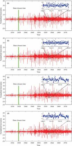
Generally speaking, it is quite important to acknowledge the fact that innovation can be considered to consist of two components at each time step: a random and a systematic component. Model structure can only manage to capture the systematic component of innovation and has nothing to do with its random component. In light of the above elaboration, normalized innovation peaks in the pre-regulation period are another issue that should be considered and analysed in Fig. 2. Contrary to the analysis presented by Rajaram and Georgakakos (1989), where the locations of these erratic values were considered possible locations for model structure inadequacy, we support the view that these anomalies in innovations are basically associated with a random component of innovation and cannot be attributed to model structure inadequacy. Given the nature of the scenarios devised in this study, we hypothesize that the model structure is expected to be inadequate after the river regulation and not before the regulation. Indeed, it can be argued that the existence of normalized innovation anomalies in the pre-regulation period is not due to the model structural issues. Rather, other factors such as the adoption of non-optimal parameters set can lead to such circumstances. Hence, the information provided by these diagrams needs to be analysed to detect possible locations of systemic changes, which has been addressed in this research.

It is also of interest and informative to report the impact of implementing a state–parameter updating approach on the ability of the model to simulate system behaviour and consequently whiten the innovations, compared to predicting the system response via LMM without using any kernel updating. For this purpose, the root mean square error (RMSE) criterion, which is based on calculating the difference between the observed and simulated values, was utilized to evaluate the model performance. Traditionally, this metric is typically calculated using the entire dataset, which can mask temporal variability in the measure of goodness of fit due to system disturbance over the simulation period (Bennett et al. 2013). Hence, evaluations were performed on a local basis (on a five-year moving window) to uncover the temporal variability in RMSE. This procedure led to the results in Table 4, where RMSE values of the two models of LMM and LMM+Dual KF, as well as their ratios, are documented for three time frames: pre-regulation, post-regulation, and the whole dataset.

Table 4. Root mean square error under the four devised scenarios.

				Streamflow RMSE^† $\left(\frac{m^3}{s}\right)$
		Pre-regulation (Year–Year)		Post-regulation (Year–Year)							Whole dataset
Scenario	Simulation model	1928 – 1932	1932 – 1937	1937 – 1942	1942 – 1947	1947 – 1952	1952 – 1957	1957 – 1962	1962 – 1967	1967 – 1972	1928 – 1972
1	LMM^⁎	15.83	18.04	22.24	29.96	33.41	37.38	27.02	31.44	23.82	26.89
	LMM+Dual KF^⁑	1.64	1.96	2.86	3.57	4.58	5.31	4.52	5.13	3.81	3.85
	RMSE Ratio^⁂	9.62	9.19	7.77	8.38	7.29	7.04	5.97	6.12	6.25	6.99
2	LMM	16.90	15.69	22.49	46.29	34.45	38.12	28.17	31.46	23.49	29.34
	LMM+Dual KF	1.77	1.81	2.93	3.88	4.75	5.46	4.66	5.18	3.85	3.94
	RMSE Ratio	9.56	8.67	7.68	11.92	7.26	6.98	6.05	6.08	6.10	7.44
3	LMM	16.74	16.66	22.08	54.08	91.64	96.63	99.10	105.50	81.22	75.36
	LMM+Dual KF	1.75	1.81	2.76	3.89	5.74	6.50	6.41	6.58	5.14	4.89
	RMSE Ratio	9.57	9.20	8.01	13.89	15.96	14.86	15.46	16.05	15.79	15.42
4	LMM	15.88	17.29	21.77	28.91	49.19	61.95	75.44	87.72	72.94	57.82
	LMM+Dual KF	1.68	1.82	2.75	3.27	4.75	5.68	5.62	6.15	4.87	4.41
	RMSE Ratio	9.47	9.50	7.91	8.84	10.36	10.91	13.42	14.27	14.98	13.12

^†RMSE = $\sqrt{\frac{1}{L}\sum _{t=1}^L{\left[Q_{sim}\left(t\right)-Q_{obs}\left(t\right)\right]}^2}$.

^⁎LMM: Simulated streamflow without kernel updating.

^⁑LMM+Dual KF: Simulated streamflow obtained by dual state–parameter updating.

^⁂RMSE ratio: $\frac{RMS{E}_{LMM}}{RMS{E}_{DualKF}}$.

Results provided in Table 4 reveal that while the RMSE ratio of the models for the first two scenarios is almost the same in both pre- and post-regulation periods, the systematic change dictated by scenarios 3 and 4 resulted in almost doubling this ratio in the post-regulation period compared to the pre-regulation period. This could be attributed to alterations of model structure resulting from systematic change imposed by the disturbance which cannot be resolved by varying the model parameters alone, as expected. However, updating model parameters in the DA framework resulted in a remarkable improvement in streamflow routing accuracy under the four devised scenarios. After imposing the disturbance, the routed streamflow generated using the updated model state and parameters outperformed the observations much more than when model state and parameters were not updated during the modelling process (see Fig. 3).

Figure 3. Visual representation of model performance for the two routing models, the LMM coupled with dual state–parameter updating kernel and LMM without coupling any kernel updating, under scenario #1 (left column) and Scenario #3 (right column) over time.

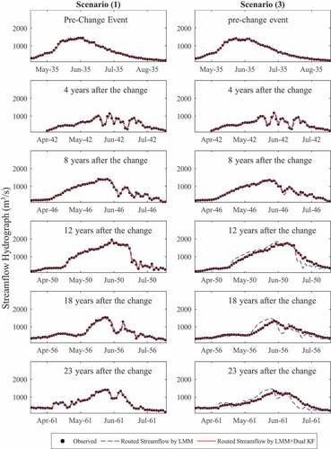
In reference to the current paper’s focus, Table 4 reveals the fact that computing a measure of goodness of fit based on the entire dataset cannot be used to delineate the time zones where the disturbance has the major impact on innovations and the model structure needs refinement to capture the system dynamics accurately. Needless to say, when it comes to choosing the time zone, the content of Table 4 in this study is gathered based on a subjective criterion, but it is quite effective to draw valid conclusions based on the numerical values of RMSE from one time zone to another. In the next section, the delineation of the representative time zone will be made automatic by resorting to a change-point detection algorithm.

3.2 Change-point detection

In the next step of the proposed methodology, the procedure described in Section 2.3.1 – namely, the MPC method – was utilized to automatically specify the number and location of change points. In this regard, the two contrast functions, defined by Equations (22)(22) $J_m\left(\mathit{\tau },\mathit{y}\right)=\sum _{k=1}^K\sum _{i={\text{taua}}_{k-1}+1}^{{\text{taua}}_k}{\left(Y_i-{\bar{Y}}_{({\text{taua}}_{k-1}+1):{\text{taua}}_k}\right)}^2$(22) and (23(23) $J_v\left(\mathit{\tau },\mathit{y}\right)=\sum _{k=1}^K\left({\text{taua}}_k-{\text{taua}}_{k-1}\right)log\left({\hat{\sigma }}_k^2\right)$(23) ), were considered to detect changes in the mean and the variance, respectively, of the four generated sequences of innovations. It is quite important to mention that in all scenarios, values of 10 and 51 were considered the upper limit of the number of segments, $K_{Max}$, to detect changes in the mean and variance, respectively. Subsequently, for each of the sequences recorded in Fig. 2, the minimum contrast value corresponding to each $K$ was individually calculated for each contrast function via implementing the first two steps of the MPC method. Figure 4 presents contrast values versus number of segments, i.e. the points $\left[pen\left(\mathit{\tau }\right)=K,J_K\right]$, when $K$ ranges from 1 up to $K_{Max}$. As shown in Fig. 4, there is a decreasing trend in contrast values, whereby the values of $J_K$ decrease as the number of segments increases, excluding the first scenario where there is no change in contrast values as the number of segments increases. When it comes to other scenarios, for change in the mean and/or change in the variance, at an early-stage of number of segments the change in contrast value is quite significant, and then the contrast values will become saturated gradually as the number of segments goes beyond a certain number (invariably called the turning point).

Figure 4. $J_K$ versus $K$ under the four devised scenarios and for the two change criteria: (1) change in the mean (left column) and (2) change in the variance (right column). The points on the convex hull (blue line) are shown with blue squares and the others are shown with red triangles.

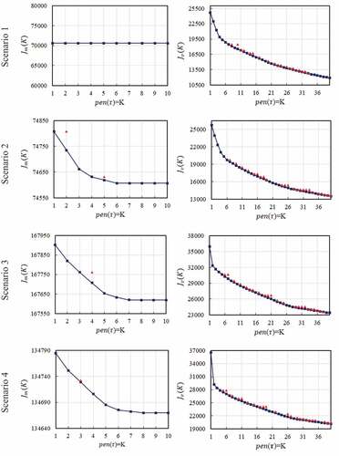
Based on the theoretical background presented by Lavielle (2005), the graphical solution for selecting the optimal number of segments is the point corresponding to the maximum curvature of the plot ($K,J_K$). This point of maximum curvature is recognized as the point for which the contrast value stops decreasing as the number of segments increases. From the viewpoint of parsimonious model structure, the contrast value has an infinite capacity for dispersion, i.e. it could decrease as much as we wish as we increase the number of segments. However, neither the current knowledge nor the model development activities could take care of this huge number of segments for model structure updating. The selection of a turning point would avoid running into this overfitting situation.

In terms of how to choose the turning point, the point of maximum curvature on the plot ($K,J_K$) can be delineated by resorting to the second-order derivative of the cited curve. This is automatically achieved through the implementation of steps 3 to 5 mentioned in Section 2.3.1. In this regard, to eliminate the effect of pseudo-curvature in determining the number of optimal segments, the convex hull of the points ($K,J_K$) was first obtained (see Fig. 4), and then the points on the convex hull were used to obtain the sequence of normalized contrasts ${\tilde{J}}_K$.This process was continued by estimating the second-order derivative of ${\tilde{J}}_K$ sequence via Equation (26)(26) $D_K={\tilde{J}}_{K-1}-2{\tilde{J}}_K+{\tilde{J}}_{K+1}$(26) . The first 10 instances of the normalized contrast sequences and their second-order derivatives for four devised scenarios and two change criteria are summarized in Table 5. Finally, considering a value of 0.75 as the threshold and comparing it with the values of $D_K$ presented in Table 5 via the logical Equation (27)(27) ${\hat{K}}_{MPC}=\mathrm{m}\mathrm{a}\mathrm{x}\left\{1\le \mathrm{K}\le K_{max}-1|D_K>S\right\}$(27) , the optimal number of segments was first specified for the two considered change criteria and all devised scenarios, and then documented in Table 6. As listed in Table 6, in the case of change in the mean, the number of change points under the four devised scenarios was 0, 3, 4, and 4, respectively. Also, for the variance change criterion, these numbers were 3, 5, 2, and 2, respectively.

Table 5. Variations of normalized contrast value and the second-order derivative against the number of segments for both the mean and variance measures.

$K$	Scenario #1				Scenario #2				Scenario #3				Scenario #4
	Changing in				Changing in				Changing in				Changing in
	Mean		Variance		Mean		Variance		Mean		Variance		Mean		Variance
	${\tilde{J}}_K$	$D_K$	${\tilde{J}}_K$	$D_K$	${\tilde{J}}_K$	$D_K$	${\tilde{J}}_K$	$D_K$	${\tilde{J}}_K$	$D_K$	${\tilde{J}}_K$	$D_K$	${\tilde{J}}_K$	$D_K$	${\tilde{J}}_K$	$D_K$
1	1	DNE^†	51	DNE	10	DNE	51	DNE	10	DNE	51	DNE	10	DNE	51	DNE
2	1	0	44.72	0.04	6.73	0	43.93	0.64	7.4	0.74	37.08	11.17	7.41	0.81	29.02	19.58
3	1	0	38.48	1.13	3.47	1.93	37.5	1.27	5.54	0.14	34.34	0.77	5.64	0	26.62	0.82
4	1	0	33.37	3.3	2.13	0.78	32.33	2.38	3.81	0	32.36	0.1	3.86	0.11	25.03	0.34
5	1	0	31.56	0.06	1.56	0	29.56	0.4	2.09	1.08	30.49	0.33	2.19	0.91	23.79	0
6	1	0	29.8	0.13	1	0.56	27.17	1.1	1.44	0.22	28.95	0	1.43	0.54	22.55	0
7	1	0	28.18	0.47	1	0	25.89	0	1.02	0.4	27.41	0	1.22	0	21.31	0.21
8	1	0	27.03	0	1	0	24.61	0.07	1	0.02	25.87	0.26	1	0.22	20.28	0
9	1	0	25.88	0.18	1	0	23.39	0	1	0	24.59	0	1	0	19.25	0.22
10	1	-	24.9	0	1	-	22.18	0.07	1	-	23.31	0.17	1	-	18.44	0

^†Does not exist.

Table 6. Number and location of detected change points based on change in the mean and variance for four devised scenarios.

Scenario	Number of change points			Location of change points (day)
	Mean		Variance	Mean		Variance
#1	0		3	-		3478
						6795
						15 994
#2	3		5	5748		2879
				6095		3134
				6485		5770
						6060
						15 994
#3	4		2	6805		3510
				8737		6790
				11 227
				13 111
#4	4		2	7190		3519
				11 227		6796
				13 843
				15 963

In light of the detected change points, it is useful and informative to touch further on the hypotheses raised in this research. In reference to change points detected in the mean and variance of the normalized innovation sequences, one can refer to these potential segments as instances of model structure inadequacy, where the model structure deserves further attention to enhance cross-validation statistics. At this stage, it makes sense to rationalize the detected change points and their synchronization with the changes dictated by each of the devised scenarios. For this purpose, the location of change points and the pathway of structural evolution in each of the scenarios are plotted in Fig. 5. As shown in Fig. 5(a–d), the pathway of structural evolution in different scenarios was well delineated and tracked by the segments detected based on changes in the mean. However, there is no significant correlation between the segments detected based on changes in the variance and dictated changes in the model structure (see Fig. 5(e–h)). It can therefore be acknowledged that the criterion of changes in the mean is a more appropriate measure for detecting systemic change and investigating its impact on model structural adequacy. Moreover, by comparing the detected points for changes in the mean under four devised scenarios, it can be argued that this change criterion has a good performance in tracking the pathway of model structure evolution for both resilient and sensitive systems. As an example, the short-term effect of river regulation on the model structure in scenario 2 (Fig. 5b) and the exponential form of the recovery pathway in scenario 3 (Fig. 5c) were accurately identified by the mean change criterion. The robustness of the proposed method in detecting different pathways of adjustment is considered another attractive advantage of the proposed algorithm. This matter was examined by comparing the results of scenarios 3 and 4. As shown in Fig. 5(c) and (d), detecting the first point with a time delay, as well as the length of the segments, both indicate a more gradual response path in scenario 4 compared to scenario 3, which is quite consistent with the nature of scenario 4.

Figure 5. The pathway of structural evolution for the four devised scenarios along with the change points detected based on the two change criteria: (1) change in the mean (left column) and (2) change in the variance (right column).

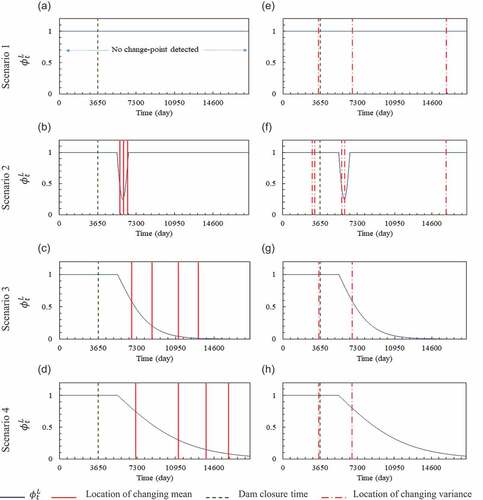
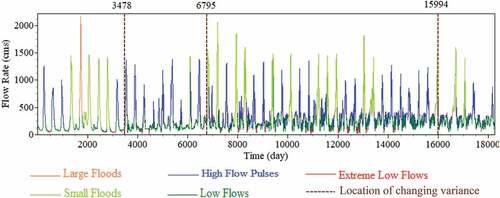
The creation of change points due to variance corresponding particularly to the first scenario points to the fact that variance is not a good measure for systemic change detection, as we would not expect any change of that nature in scenario 1. The cause of changes in the variance of the normalized innovation sequences can be attributed to other factors irrelevant to the model structure inadequacy. Acknowledging the streamflow variability as a system stimulus, historical cycles of the environmental flow components, i.e. low flows, extreme low flows, high-flow pulses, small floods, and large floods for the entire flow simulation period, were plotted along with the variance change points under scenario 1 to investigate the cause of change in the variance as it relates to streamflow variability (see Fig. 6). As discussed, the contrast function in the case of changes in the variance has been developed based on the constant mean assumption. Hence, variance change points for scenario 1, which satisfies this assumption well, were considered as the reference to investigate this issue. As shown in Fig. 6, different clusters of flood series (e.g. periods of high-flow pulses, small floods, and large floods) correspond to segments detected based on the variance change criterion. Hence, a significant correlation can be acquired between the two, i.e. streamflow variability and detected segments based on change in variance. In light of the above elaboration, it seems necessary to distinguish between systemic change and innovation fluctuations due to temporary changes in system input as it relates to model structure inadequacy.

Figure 6. Temporal variability of environmental flow components along with the locations of change points in the variance for scenario #1.

4 Conclusions

This study was undertaken to investigate the possibility of detecting systemic changes within a typical river reach over a given time frame due to its possible and potential regulation. For this purpose, an objective two-step change detection algorithm was developed. The major novelty of the contribution here was to generate a sequence of synthetic normalized innovation via an appropriate model coupled with an updating filter in the first step and then introduce this sequence as input to the change detector in the second step. To investigate the robustness of the proposed methodology, four numerical experiments were devised based on the principles of geomorphic response to a disturbance event. The following conclusions can be drawn from the current study:

Visual examination of generated normalized innovation sequences shows that the characteristics of the innovation sequence are a good measure to detect systemic changes and the inability of the selected model structure to mimic the deterministic features inherent in data. However, to make a reliable and objective judgement regarding model structure inadequacy, it is crucial to analyse the evolution of information provided by the sequence of innovations.

Generally, the performance of the proposed methodology in detecting systemic changes depends on the change criterion chosen. Our investigation of the results of numerical experiments clearly indicates the importance of the change criterion selection in delineating and tracking the pathway of structural evolution.

The rationalization of the detected change points highlights the fact that the mean change criterion is a more appropriate measure for detecting the systemic change and investigating its impact on model structural adequacy. However, the variance change criterion is more appropriate for investigating streamflow variability and detecting periodic behaviour in the inflow hydrograph.

The overall conclusion is that because the proposed methodology benefits from an objective decision system to investigate the functional behaviour of the system under post-disruption conditions, it could be regarded as a suitable alternative for detecting systemic change and investigating its impact on model structural adequacy.

The employment of a relatively simple hydrological routing model, i.e. LMM, as the initial model can be considered one of the limitations of the proposed method. Another potential limitation regarding the current study is that the implementation of the proposed methodology benefits from synthetic data as opposed to real field data. Furthermore, another pitfall associated with the proposed approach is that among the three groups of potential change drivers, i.e. human activities in the river corridor itself, land-use change, and climate change, only river regulation was considered as the system driver. Hence, it is recommended that the proposed methodology be implemented in a real river corridor, where any of these factors and/or a combination of them can act as the system stimulus. Recognizing the importance of local evaluation of measures of goodness of fit in revealing significant divergent behaviour over the simulation period, another recommended research avenue is to investigate the performance of the proposed method as an automatic grouping method. In this case, the proposed method could be used to delineate representative time zones wherein measures of goodness of fit remain invariant for possible model structure updating from one grouping reach to another.

Disclosure statement

No potential conflict of interest was reported by the authors.

References

- Akaike, H., 1974. A new look at the statistical model identification. IEEE Transactions on Automatic Control, 19 (6), 716–723. doi:10.1109/TAC.1974.1100705
- Allen, J.R.L., 1974. Reaction, relaxation and lag in natural sedimentary systems: general principles, examples and lessons. Earth-Science Reviews, 10 (4), 263–342. doi:10.1016/0012-8252(74)90109-3
- Arrigoni, A.S., Greenwood, M.C., and Moore, J.N., 2010. Relative impact of anthropogenic modifications versus climate change on the natural flow regimes of rivers in the Northern Rocky Mountains, United States. Water Resources Research, 46 (12). doi:10.1029/2010WR009162
- Bellman, R., 1966. Dynamic programming. Science, 153 (3731), 34–37. doi:10.1126/science.153.3731.34
- Bennett, N.D., et al., 2013. Characterising performance of environmental models. Environmental Modelling and Software, 40, 1–20. doi:10.1016/j.envsoft.2012.09.011
- Brierley, G.J. and Fryirs, K.A., 2013. Geomorphology and river management: applications of the river styles framework. Chichester, UK: John Wiley & Sons, Ltd.
- Buechel, M., Slater, L., and Dadson, S., 2022. Hydrological impact of widespread afforestation in Great Britain using a large ensemble of modelled scenarios. Communications Earth & Environment, 3 (1), 1–10. doi:10.1038/s43247-021-00334-0
- Butts, M.B., et al., 2004. An evaluation of the impact of model structure on hydrological modelling uncertainty for streamflow simulation. Journal of Hydrology, 298 (1–4), 242–266. doi:10.1016/j.jhydrol.2004.03.042
- Ciria, T.P., Labat, D., and Chiogna, G., 2019. Detection and interpretation of recent and historical streamflow alterations caused by river damming and hydropower production in the Adige and Inn River basins using continuous, discrete and multiresolution wavelet analysis. Journal of Hydrology, 578, 124021. doi:10.1016/j.jhydrol.2019.124021
- Cunge, J.A., 1969. On the subject of a flood propagation computation method (Musklngum method). Journal of Hydraulic Research, 7 (2), 205–230. doi:10.1080/00221686909500264
- Feng, P., Wu, J., and Li, J., 2019. Changes in flood characteristics and the flood driving mechanism in the mountainous Haihe River Basin, China. Hydrological Sciences Journal, 64 (16), 1997–2005. doi:10.1080/02626667.2019.1619931
- Fryirs, K.A., 2017. River sensitivity: a lost foundation concept in fluvial geomorphology. Earth Surface Processes and Landforms, 42 (1), 55–70. doi:10.1002/esp.3940
- Georgakakos, A.P., Georgakakos, K.P., and Baltas, E.A., 1990. A state‐space model for hydrologic river routing. Water Resources Research, 26 (5), 827–838.
- Graf, W.L., 1977. The rate law in fluvial geomorphology. American Journal of Science, 277 (2), 178–191. doi:10.2475/ajs.277.2.178
- Graf, W.L., 2006. Downstream hydrologic and geomorphic effects of large dams on American rivers. Geomorphology, 79 (3–4), 336–360. doi:10.1016/j.geomorph.2006.06.022
- Gustafsson, F., 2000. Adaptive filtering and change detection. Vol. 1, New York: Wiley.
- Hall, J., et al., 2014. Understanding flood regime changes in Europe: a state-of-the-art assessment. Hydrology and Earth System Sciences, 18 (7), 2735–2772. doi:10.5194/hess-18-2735-2014
- Hasanvand, K., Hashemi, M.R., and Abedini, M.J., 2013. Development of an accurate time integration technique for the assessment of Q-based versus h-based formulations of the diffusion wave equation for flow routing. Journal of Hydraulic Engineering, 139 (10), 1079–1088. doi:10.1061/(ASCE)HY.1943-7900.0000773
- Haykin, S., 2004. Kalman filtering and neural networks. Vol. 47. New York: John Wiley & Sons.
- Hendricks Franssen, H.J. and Kinzelbach, W., 2008. Real‐time groundwater flow modeling with the ensemble Kalman filter: joint estimation of states and parameters and the filter inbreeding problem. Water Resources Research, 44 (9). doi:10.1029/2007WR006505
- Kalman, R.E., 1960. A new approach to linear filtering and prediction problems. Journal of Basic Engineering, 82 (1), 35–45. doi:10.1115/1.3662552
- Killick, R., Fearnhead, P., and Eckley, I.A., 2012. Optimal detection of changepoints with a linear computational cost. Journal of the American Statistical Association, 107 (500), 1590–1598. doi:10.1080/01621459.2012.737745
- Kim, D.H. and Georgakakos, A.P., 2014. Hydrologic routing using nonlinear cascaded reservoirs. Water Resources Research, 50 (8), 7000–7019. doi:10.1002/2014WR015662
- Lavielle, M., 2005. Using penalized contrasts for the change-point problem. Signal Processing, 85 (8), 1501–1510. doi:10.1016/j.sigpro.2005.01.012
- Leisenring, M. and Moradkhani, H., 2012. Analyzing the uncertainty of suspended sediment load prediction using sequential data assimilation. Journal of Hydrology, 468, 268–282. doi:10.1016/j.jhydrol.2012.08.049
- Mathews, R. and Richter, B.D., 2007. Application of the indicators of hydrologic alteration software in environmental flow setting 1. JAWRA Journal of the American Water Resources Association, 43 (6), 1400–1413. doi:10.1111/j.1752-1688.2007.00099.x
- Matteson, D.S. and James, N.A., 2014. A nonparametric approach for multiple change point analysis of multivariate data. Journal of the American Statistical Association, 109 (505), 334–345. doi:10.1080/01621459.2013.849605
- Mazzoleni, M., et al., 2018. Real-time assimilation of streamflow observations into a hydrological routing model: effects of model structures and updating methods. Hydrological Sciences Journal, 63 (3), 386–407. doi:10.1080/02626667.2018.1430898
- McCarthy, G.T., 1938. The unit hydrograph and flood routing. In Proceedings of conference of North Atlantic Division, US Army Corps of Engineers. Concord, MA, 608–609.
- Meditch, J.S., 1969. Stochastic optimal linear estimation and control. New York: McGraw-Hill.
- Moradkhani, H., et al., 2005. Dual state–parameter estimation of hydrological models using ensemble Kalman filter. Advances in Water Resources, 28 (2), 135–147. doi:10.1016/j.advwatres.2004.09.002
- Pathiraja, S., et al., 2016. Hydrologic modeling in dynamic catchments: a data assimilation approach. Water Resources Research, 52 (5), 3350–3372. doi:10.1002/2015WR017192
- Petts, G.E., 1987. Time-scales for ecological change in regulated rivers. In: J.F. Craig and J.B. Kemper, eds. Regulated streams. Boston, MA: Springer, 257–266.
- Phillips, J.D. and Van Dyke, C., 2016. Principles of geomorphic disturbance and recovery in response to storms. Earth Surface Processes and Landforms, 41 (7), 971–979. doi:10.1002/esp.3912
- Poeppl, R.E., Keesstra, S.D., and Maroulis, J., 2017. A conceptual connectivity framework for understanding geomorphic change in human-impacted fluvial systems. Geomorphology, 277, 237–250. doi:10.1016/j.geomorph.2016.07.033
- Poff, N.L., et al., 1997. The natural flow regime. BioScience, 47 (11), 769–784. doi:10.2307/1313099
- Polhill, J.G., et al., 2016. Modelling systemic change in coupled socio-environmental systems. Environmental Modelling and Software, 75, 318–332. doi:10.1016/j.envsoft.2015.10.017
- Rajaram, H. and Georgakakos, K.P., 1989. Recursive parameter estimation of hydrologic models. Water Resources Research, 25 (2), 281–294. doi:10.1029/WR025i002p00281
- Reichle, R.H., Crow, W.T., and Keppenne, C.L., 2008. An adaptive ensemble Kalman filter for soil moisture data assimilation. Water Resources Research, 44 (3). doi:10.1029/2007WR006357
- Schwarz, G., 1978. Estimating the dimension of a model. The Annals of Statistics, 6 (2), 461–464. doi:10.1214/aos/1176344136
- Sharma, S., Swayne, D.A., and Obimbo, C., 2016. Trend analysis and change point techniques: a survey. Energy, Ecology and Environment, 1 (3), 123–130. doi:10.1007/s40974-016-0011-1
- Simon, D., 2006. Optimal state estimation: Kalman, H infinity, and nonlinear approaches. Hoboken, NJ: Wiley-Interscience.
- Singh, V.P. and Scarlatos, P.D., 1987. Analysis of nonlinear Muskingum flood routing. Journal of Hydraulic Engineering, 113 (1), 61–79. doi:10.1061/(ASCE)0733-9429(1987)113:1(61)
- Slater, L.J., et al., 2021. Nonstationary weather and water extremes: a review of methods for their detection, attribution, and management. Hydrology and Earth System Sciences, 25 (7), 3897–3935. doi:10.5194/hess-25-3897-2021
- Slater, L.J., Singer, M.B., and Kirchner, J.W., 2015. Hydrologic versus geomorphic drivers of trends in flood hazard. Geophysical Research Letters, 42 (2), 370–376. doi:10.1002/2014GL062482
- Smith, P.J., et al., 2013. Data assimilation for state and parameter estimation: application to morphodynamic modelling. Quarterly Journal of the Royal Meteorological Society, 139 (671), 314–327. doi:10.1002/qj.1944
- Todini, E., 1978. Mutually interactive state-parameter (MISP) estimation. In: Proceedings of AGU Chapman conference, 22–24 May 1978 Pittsburgh, PA.
- Vatankhah, A.R., 2021. The lumped Muskingum flood routing model revisited: the storage relationship. Hydrological Sciences Journal, 66 (11), 1625–1637. doi:10.1080/02626667.2021.1957475
- Verstegen, J.A., et al., 2016. Detecting systemic change in a land use system by Bayesian data assimilation. Environmental Modelling and Software, 75, 424–438. doi:10.1016/j.envsoft.2015.02.013
- Vrugt, J.A. and Sadegh, M., 2013. Toward diagnostic model calibration and evaluation: approximate Bayesian computation. Water Resources Research, 49 (7), 4335–4345. doi:10.1002/wrcr.20354
- Williams, G.P. and Wolman, M.G., 1984. Downstream effects of dams on alluvial rivers. Vol. 1286. Washington, DC: US Government Printing Office.
- Wu, B., Zheng, S., and Thorne, C.R., 2012. A general framework for using the rate law to simulate morphological response to disturbance in the fluvial system. Progress in Physical Geography, 36 (5), 575–597. doi:10.1177/0309133312436569
- Zhou, C., et al., 2019. Comparative analysis of nonparametric change-point detectors commonly used in hydrology. Hydrological Sciences Journal, 64 (14), 1690–1710. doi:10.1080/02626667.2019.1669792
- Zuo, Q., et al., 2019. Quantitative research on the water ecological environment of dam-controlled rivers: case study of the Shaying River, China. Hydrological Sciences Journal, 64 (16), 2129–2140. doi:10.1080/02626667.2019.1669794