A hydrologic and river ice modelling framework for assessing ungauged sub-basin streamflow impact in a large cold-region river basin

ABSTRACT

Modelling snow- and ice-affected streamflow in cold regions is challenging. Neglecting the streamflow from ungauged regions/sub-basins of a river basin in the inflow boundaries of a river ice model adds further uncertainties. This study combined a river ice model (River1D) with a hydrological model (Soil and Water Assessment Tool, SWAT) to investigate the impacts of ungauged sub-basin streamflow on peak flow simulation under both open water and river ice breakup conditions in the Peace River Basin (PRB). Results showed that ungauged sub-basins of the PRB can greatly affect peak flow simulation of the River1D for both open water and river ice breakup events, especially for flood events. Although they represent only about 26.54% of the whole modelled area in the PRB, the SWAT model simulated results show that the ungauged sub-basins can contribute nearly 50% of peak flow for the open water and river ice breakup flood events.

KEYWORDS:

• ungauged basins
• river ice breakup
• river ice model
• flood
• SWAT
• Peace River Basin

Editor A. Fiori; Associate Editor O. Makarieva

1 Introduction

Disastrous river floods have caused fatalities, displacement, and huge economic losses globally (Merz et al. 2021), and it is projected that more global population will be exposed to floods in the future (Tellman et al. 2021). In addition to heavy rainfall, flood dynamics could also be driven by snowmelt and river ice processes in cold region rivers (Das et al. 2020, Mishra et al. 2022). Snow and ice are major components of the hydrological regime in northern latitudes, and their combined effects can greatly affect streamflow. River ice breakup can be thermally or mechanically driven. A thermal breakup occurs when the streamflow remains relatievly steady over several warm days. The ice cover deteriorates in place with minimal movement. Significantly increased streamflow due to rapid melting of large snowpacks can result in mechanical breakup of a river ice cover (Beltaos and Prowse 2009). This results in increased hyrodynamic forces, which lift and dislodge an intact ice cover before any significant deterioriation occurs. Unlike a thermal breakup, a mechanical breakup is highly dynamic and often associated with ice runs. Ice jams form when ice runs are arrested by downstream intact ice cover or constrictions such as bridge piers and islands (Beltaos 2008). Breakup ice jams can lead to fast-rising water levels and cause severe flooding even at lower streamflow as compared to open water floods (Beltaos and Prowse 2001, Burrell et al. 2021). Ice jam-caused damages in North America amount to nearly 300 million CAD annually on average (French 2017).

The hydrological and hydraulic modelling framework has been widely used for flood forecasting and risk assessment (Bonnifait et al. 2009, Nguyen et al. 2016, Grimaldi et al. 2019, Li et al. 2019b), but these previous studies mostly focused on open water floods. Ice-induced floods are much more complex and chaotic (Turcotte et al. 2019). Hydrological models generally are not equipped to simulate river ice processes, and thus can lead to significant uncertainties and errors when attempting to simulate ice-induced floods through parameter calibration. It is imperative to account for the effects of ice in order to correctly simulate the river hydraulic conditions. This necessitates the utilization of specialized hydraulic models capable of simulating various river ice processses, which will be referred to as river ice models henceforth. Examples of river ice models include River1D (Blackburn and She 2019), Comprehensive River Ice Simulation System Program (CRISSP) (Chen et al. 2006, Liu et al. 2006), Mike-Ice (Thériault et al. 2010), and RIVICE (Lindenschmidt 2017). Existing river ice models simulate the onset of mechanical breakup using empirical criteria or based on user-specified breakup timing and locations (Ye and She 2021). Several studies have used a hydrological model in conjunction with a river ice model to assess future ice regime and ice-jam flood risk. Timalsina et al. (2015) evaluated the impact of climate change on a river ice regime using the indices of water temperature, frazil ice concentration and ice cover extent in a medium-scale regulated river in Norway using Mike-Ice and the Hydrologiska Byråns Vattenbalansavdelning (HBV) hydrological model. Lindenschmidt et al. (2019) and Das et al. (2020) used RIVICE and Modélisation Environnementale communautaire - Surface Hydrology (MESH) hydrological models for operational real-time and future ice jam flood hazard assessment and flood mapping. The focus was on the simulation of water level profiles caused by ice jams using a stochastic modelling approach. More work is needed to improve the capability of the hydrological and river ice modelling framework for simulating the comprehensive processes of snow- and ice-induced floods in cold-region river basins.

Many drainage basins of the world are ungauged or poorly gauged (Sivapalan 2003, Sivapalan et al. 2003, Mishra and Coulibaly 2009). Even for basins with a good number of well-distributed gauge stations, flow from certain regions or sub-basins can still be ungauged. For example, the hydrometric stations on tributaries are often located at a distance upstream of the confluence to the mainstream, and thus the streamflow from the area between the hydrometric station and the confluence is ungauged. Some catchments or sub-basins in a river basin are often not gauged as they only have significant flows during flood periods. The total ungauged sub-basins usually represent a significant portion of a river basin (Viglione et al. 2013, Dessie et al. 2015). However, the ungauged catchment streamflow is not easy to estimate and often not taken into account in the inflow boundaries of hydraulic models (Zhang et al. 2017), which can introduce significant uncertainies and/or errors when simulating flood events.

Estimation or prediction of ungauged streamflow is a challenging research field (Sivapalan 2003, Hrachowitz et al. 2013, Guo et al. 2021). The International Association of Hydrological Sciences (IAHS) launched the initiative for Predictions in Ungauged Basins (PUB) in 2003 to stimulate the development of new and advanced predictive approaches (Sivapalan et al. 2003), and numerous studies have been carried out since then (Zhang and Chiew 2009, Parajka et al. 2013, Salinas et al. 2013, Viglione et al. 2013, Booker and Woods 2014, Zelelew and Alfredsen 2014, Pagliero et al. 2019, Singh et al. 2022). Most of these studies aim to identify donor gauged catchments that are hydrologically similar to the target ungauged catchments, and then transfer information (e.g. streamflow or calibrated hydologic model parameters) from gauged catchments to ungauged catchments. This process is generally refered as regionalization (Blöschl and Sivapalan 1995, He et al. 2011). The simplest regionalization method is probably the draninage-area ratio (DAR) method, which generally estimates the streamflow at an ungauged catchment using the streamflow information of a nearby gauged catchment and the ratio of the drainage areas of the donor and target catchments (McCuen and Levy 2000, Emerson et al. 2005, Asquith et al. 2006, Gianfagna et al. 2015, Ergen and Kentel 2016, Li et al. 2019a). The DAR method can produce reasonable results when the ungauged catchment and its donor gauged catchment have homogeneous hydrological characteristics (Ergen and Kentel 2016). The more sophisticated and widely used regionalization methods are based on hydrological models (Parajka et al. 2013, Razavi and Coulibaly 2013, Guo et al. 2021), which generally use hydrological model parameters calibrated for the donor gauged catchment(s) to derive the model parameters for the target ungauged catchment, and estimate or predict the ungauged streamflow. However, it is not uncommon that these methods produce unsatisfactory simulation results and low prediction accuracy due to large heterogeneity of land surface conditions, spatial and temporal variability of climatic inputs, unclear hydrological similarity indicators, and uncertainties arising from model structures and calibrations (Sivapalan 2003, Hrachowitz et al. 2013, Guo et al. 2021).

A hydraulic model can be a useful tool to verify the hydrological model simulated ungauged catchment streamflow. For example, Liu et al. (2015) coupled the Soil and Water Assessment Tool (SWAT) hydrological model and the XSECT hydraulic model for estimating streamflow and water levels for ungauged sub-basins in the Red River Basin (US portion). The SWAT model was used to estimate streamflow to provide inflows to the XSECT model, which was then used to simulate water levels and water surface areas. With a comparison to their observed values extracted from satellites, the XSECT model results provided a verification of the ungauged streamflow simulated by SWAT. Zhang et al. (2017) used the SWAT model to simulate the streamflow of the ungauged zones in the Poyang Lake Basin, and the verification was achieved using the Delft3D hydraulic model through comparing the simulated flow and lake water levels with the observed ones. Although there are numerous studies on estimating/predicting and verifying the ungauged streamflow using the hydrological and hydraulic modelling framework, the effects of ungauged sub-basins on peak flow, especially snow- and ice-induced peak flow during river breakup in large cold-region river basins, remain to be explored. The hydrological and river ice modelling framework offers good potential for this purpose.

The objectives of this study are to (1) assess ungauged sub-basin streamflow estimation methods (i.e. the simple drainage-area ratio method and sophisticated hydrological model); (2) investiagte the impacts of ungauged sub-basins on peak flow simualtion under open water and river ice breakup conditions; and (3) analyse the peak flow contributions of the gauged and ungauged sub-basins for open water and river ice breakup events. To achieve these objectives, a modelling framework was established utilizing the public-domain hydrological model SWAT and the hydraulic/river ice model River1D. The SWAT model was used to delineate a river basin into gauged and ungauged sub-basins, estimate the gauged and ungauged sub-basin streamflow, and provide inflow boundaries for the river ice model. The River1D model was used to simulate mainstream flow during open water and river ice breakup periods. The framework was applied to the Peace River Basin (PRB), a large cold-region watershed in western Canada. Two open water and three river ice breakup periods were simulated, and the impacts of ungauged sub-basin streamflow on peak flow of these periods were evaluated.

2 Data and methodology

The process for estimating and evaluating the ungauged sub-basin streamflow in a river basin is shown in Fig. 1. It includes: (1) delineating a basin into gauged and ungauged sub-basins, and simulating the streamflow for the gauged and ungauged sub-basins using the hydrological model; (2) coupling the hydrological model outputs and river ice model inputs; and (3) evaluating ungauged sub-basins’ streamflow with the river ice and hydrological models. The second step of model coupling is achieved by (a) allocating ungauged sub-basins into various inflow boundaries for the river ice model, (b) estimating ungauged sub-basin streamflow using the DAR method and/or the hydrological model, and (c) setting up different inflow boundary scenarios based on how the ungauged sub-basin streamflow is estimated. In the modelling framework, the river ice model-simulated results provide feedback for the hydrological model. For Inflow boundary scenario (IBS)3 in Fig. 1, if the river ice model-simulated streamflow and/or water level on the mainstream at certain hydrometric stations did not agree with the observed values, the hydrological model was recalibrated to improve the estimation of the streamflow from ungauged sub-basins. This was an iterative process, carried out until the hydrological model could provide satisfactory simulated streamflow in ungauged sub-basins for the river ice model.

Figure 1. Flowchart for estimating and evaluating ungauged sub-basin streamflow in a river basin through combined use of hydrological and river ice models.

2.1 Study area and data

The Peace River originates in the Rocky Mountains, flowing ~1923 km through British Columbia and northern Alberta before joining with the Athabasca River and forming the Slave River. The PRB has an area of approximately 306 000 km², with elevations ranging from approximately 3286 m to about 200 m from upstream to downstream (Fig. 2). In Fig. 2, the area enclosed by the black line indicates the area modelled by the hydrological model in this study (an area of around 277 286 km²). The modelled reach in the river ice model (blue line in Fig. 2) extends from Hudson Hope to approximately 100 km downstream of Fort Vermilion, for a total length of 932 km. The river stationing is the distance from the W.A.C. Bennett Dam.

Figure 2. Map of the Peace River Basin and study reach, with the location of the hydrometric gauge stations used in this study.

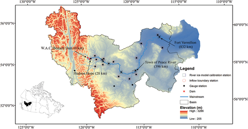
Streamflow data are available from the Water Survey of Canada (WSC). Twenty-three gauge stations were used for calibrating and validating the hydrological model, shown as black dots in Fig. 2. Of these stations, 14 (circled in red) were used to determine the inflow and tributary inflow boundary conditions for the river ice model. Water levels from seven gauge stations located on the Peace River (hollow black squares) were used for calibrating and validating the river ice model. Details of these gauge stations are summarized in Table 1.

Table 1. Hydrometric stations in the Peace River Basin used in this study.

ID	Station	Station name	Longitude	Latitude	Data used	Usage
1	07EF001	Peace River at Hudson Hope	−121.91	56.03	Flow	Hydrological model calibration/validation and river ice model inflow boundary
2	07FA006	Halfway River near Farrell Creek	−121.63	56.25	Flow
3	07FB008	Moberly River near Fort St. John	−121.37	56.09	Flow
4	07FB001	Pine River at East Pine	−121.21	55.72	Flow
5	07FC001	Beatton River near Fort St. John	−120.7	56.28	Flow
6	07FD001	Kiskatinaw River near Farmington	−120.56	55.96	Flow
7	07FD009	Clear River near Bear Canyon	−119.68	56.31	Flow
8	07GJ001	Smoky River at Watino	−117.62	55.72	Flow
9	07GE001	Wapiti River near Grande Prairie	−118.8	55.07	Flow
10	07HA003	Heart River near Nampa	−117.13	56.06	Flow
11	07HC001	Notikewin River at Manning	−117.62	56.92	Flow
12	07HF002	Keg River at Highway No. 35	−117.63	57.75	Flow
13	07JF003	Ponton River above Boyer River	−116.26	58.46	Flow
14	07JD002	Wabasca River at Highway No. 88	−115.39	57.88	Flow
15	07EE007	Parsnip River above Misinchinka River	−122.91	55.08	Flow	Hydrological model calibration/validation
16	07FD006	Saddle River near Woking	−118.7	55.64	Flow
17	07GH002	Little Smoky River near Guy	−117.16	55.46	Flow
18	07FA004	Peace River above Pine River	−120.82	56.2	Flow an Level	Hydrological model and river ice model calibration/validation
19	07FD002	Peace River near Taylor	−120.67	56.14	Flow and Level
20	07FD010	Peace River above Alces River	−120.06	56.13	Flow and Level
21	07FD003	Peace River at Dunvegan Bridge	−118.61	55.92	Flow and Level
22	07HA001	Peace River at Peace River	−117.31	56.25	Flow and Level
23	07HF001	Peace River at Fort Vermilion	−116.03	58.39	Flow and Level
24	07FD901	Peace River above Smoky River Confluence	−117.44	56.16	Level	River ice model calibration/validation

2.2 Hydrological model

The SWAT2012 model, a semi-distributed and river basin scale model (Arnold et al. 1998, Neitsch et al. 2011), was used to divide the river basin into gauged and ungauged sub-basins, and to simulate streamflow. The model delineates a watershed into sub-basins, which is further divided into hydrological response units (HRUs). An HRU is a combination of unique soil, land cover and slope. The watershed delineation is based on the digital elevation model (DEM). The ArcSWAT interface for the SWAT2012 model can automatically create streams and outlets for the watershed based on the DEM (Winchell et al. 2013). However, outlets are not necessarily situated at the locations of the actual gauge stations, and some outlets are too concentrated due to the combined uncertainties of the DEM and the outlet generation algorithm used in ArcSWAT. The ArcSWAT interface allows users to manually edit the outlets for the sub-basins during watershed delineation. In this study, unnecessary outlets were deleted to avoid overly dense outlet locations and to reduce the model complexity. Meanwhile, additional outlets were added based on the locations of the gauge stations used in this study for delineating the gauged and ungauged sub-basins, as well as for model calibration (see Table 1). Detailed model set-up and calibration have been previously conducted for the PRB (Chen et al. 2023).

The SWAT model was calibrated from 2004 to 2013 based on the widely used Sequential Uncertainty Fitting program (SUFI-2) of SWAT-Calibration Uncertainty Procedures (CUP) (Abbaspour 2015). Daily streamflow values at the 23 selected stations shown in Table 1 were used, and daily snow water equivalent (SWE) values at 23 point stations near the flow stations were obtained from the ERA5 reanalysis data (Hersbach et al. 2020). Various calibration schemes were tested, including the application of two commonly used efficiency coefficients, the Nash-Sutcliffe efficiency (NS) and a modified version of the efficiency criterion (bR²) defined by Krause et al. (2005), as objective functions for both single-variable (streamflow) and multiple-variable (streamflow and SWE) calibrations.

The simulated ungauged sub-basin streamflow values were subsequently employed as inputs to the river ice model and evaluated using streamflow and water level data. It was found that the bR² performed better in capturing the peak flows and when there were many missing values in observed streamflow data. As the peak flow during open water and river ice breakup periods were the focus of this study and some of the flow stations on the tributaries have many missing values, bR² was used as the objective function in SUFI-2 of SWAT-CUP. Consistent with the findings of Chen et al. (2023), the utilization of multi-variable calibration using streamflow and SWE improved prediction accuracy for snow-affected spring streamflow.

2.3 River ice model

The open water and river ice hydraulic modelling was conducted with the University of Alberta’s public-domain River1D model. The model originated as a hydrodynamic model (Hicks and Steffler 1990, 1992), and was gradually expanded to simulate various river ice processes (She and Hicks 2006, Andrishak and Hicks 2008, She et al. 2009, Blackburn and She 2019). River1D can simulate the mechanical breakup of an ice cover via different breakup criteria; a systematic evaluation is provided by Ye and She (2021). However, validation of these breakup criteria is limited. To reduce the uncertainties of simulating the progression of ice breakup, and because the ice front location on the Peace River has been observed relatively frequently, ice cover breakup was not modelled with a breakup criterion in this study, but rather with the observed ice front locations provided to the River1D model. Ice front locations during river breakup were mainly obtained from the River Ice Observation Reports Archive of the Government of Alberta (https://rivers.alberta.ca/#), supplemented by information extracted from the Landsat Data (https://www.usgs.gov/landsat-missions/data).

A static ice cover was assumed to be initially present in the study reach, mimicking the pre-breakup condition. The initial ice thickness was set according to the observed stable ice thickness available at two WSC gauge stations (Peace River at Peace River and Peace River at Peace Point) on the Peace River from the Canadian River Ice Database (De Rham et al. 2020). At each time step, the model checked where the ice front was located. Following Ye and She (2021), a transition zone of five channel widths was assumed to exist between the freely flowing broken ice and the intact ice cover, within which the ice offers reduced resistance to flow. The ice velocity within the transition zone was assumed to decrease linearly from the open water velocity to zero from upstream to downstream.

The geometric model is a combination of surveyed and approximated cross-sections (Blackburn and Hicks 2002, Ye and She 2021). Sub-daily discharge data were requested from Environment and Climate Change Canada (ECCC) and used as inflow boundary conditions at the upstream end of the study reach and incoming tributaries (see Table 1). When values are missing in the sub-daily dataset, which was mainly the case for small tributaries and during low flow periods, the daily streamflow value (publicly available from the WSC hydrometric database) on the same day was used. When daily data are used as inflows (e.g. the streamflow estimated using the hydrological model), River1D interpolates between two adjacent daily values to obtain the value at the computational time step. No water level data were available at the downstream boundary of the modelled reach, but since it is about 100 km downstream of the reach of interest (i.e. Hudson Hope to Fort Vermillion), a constant water level boundary could be assumed without impacting the hydraulic conditions in the reach of interest.

Sub-daily data on streamflow and water levels at seven hydrometric stations on the Peace River (see Table 1), requested from ECCC, were employed to calibrate the river ice model for open water and river ice breakup events. Model calibration for open water events was completed by adjusting the main channel bed roughness values of the study reach. The bed roughness values calibrated for the open water periods were kept the same when simulating the breakup period, and the ice roughness values were calibrated. The model performance was evaluated using NS and the coefficient of determination (R²), with the NS indicating how well a model predicts the observed data and R² describing the degree of collinearity between simulated and measured data (Moriasi et al. 2007). The range of R² is 0 to 1 while NS ranges from −∞ to 1, with the perfect value of both being 1. In addition to these two indices, the peak flow difference was also used to evaluate the model performance.

2.4 Model coupling

2.4.1 Delineation of gauged and ungauged sub-basins

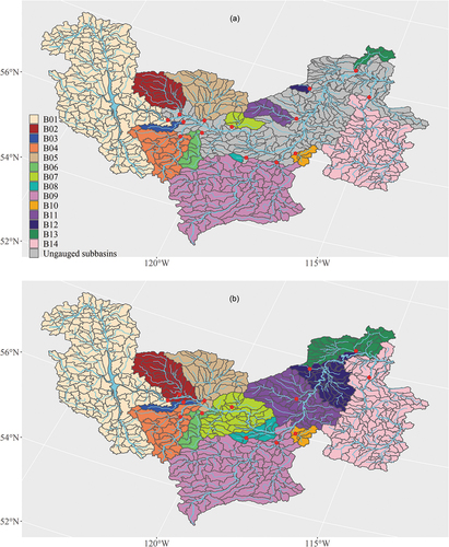
The PRB was delineated into 818 sub-basins using the SWAT model. The 14 hydrometric stations (Table 1) used to set the inflow boundaries for the river ice model were used to distinguish the ungauged sub-basins from gauged sub-basins (Fig. 3a). The drainage area of a hydrometric station contains all the sub-basins upstream of this station, and the 14 inflow boundary zones (colored area) for the River1D model correspond to the 14 hydrometric stations. The remaining (grey) area of the PRB covers all the ungauged sub-basins, which takes up about 26.54% of the whole modelled area. The ungauged sub-basins were manually allocated into the nearby 14 inflow boundary zones so that the impacts of ungauged sub-basin streamflow on the inflow boundaries of the river ice model could be evaluated (see Fig. 3b). Manual allocation was mainly based on the final outlet location of each ungauged sub-basin relative to the mainstream and the locations of the mainstream gauge stations.

Figure 3. Delineated sub-basins of Peace River Basin (a) gauged inflow boundary zones (various colours) and ungauged sub-basins (grey); (b) ungauged sub-basins allocated into 14 inflow boundary zones.

2.4.2 Ungauged sub-basin streamflow estimation

The inflow boundary hydrometric stations on the tributaries (Table 1) are not located right at the confluence to the Peace River (see Fig. 3). The streamflow from the area between the tributary gauge and the confluence therefore is not considered if the gauge data are directly used as the inflow boundaries for the river ice model. To account for these ungauged flows, Hicks (1996) used a set of multiplication factors from Taggart (1995) to adjust the tributary inflow boundaries of the Peace River when simulating open water flood events using the River1D model. These multiplication factors were computed based on the ratio of the catchment area at the confluence to the catchment area at the tributary gauge (i.e. the DAR method). These multiplication factors were used in this study as the base scenario (S1 in Table 2). Not all inflow boundaries were adjusted by the multiplication factors in the study of Hicks (1996), i.e. S1 only partly considers ungauged areas between the tributary gauge and the outlet to the main river. Additionally, there are still some ungauged sub-basins that tributary gauge stations cannot cover even if every tributary gauge station is located at the outlet to the main river. S1 also does not consider these ungauged sub-basins.

Table 2. The three scenarios of inflow boundaries of River1D.

Boundary	Station	Gauged area (km^2)	Ungauged area (km^2)	Scenario 1 (S1)	Scenario 2 (S2)	Scenario 3 (S3)
B01	07EF001	70 042.28	0	1*Qgauged01	1*Qgauged01	1*Qgauged01
B02	07FA006	9238.09	2830.87	1*Qgauged02	1.306*Qgauged02	1.306*Qgauged02
B03	07FB008	1505.69	433.54	1.4*Qgauged03	1.288*Qgauged03	1.288*Qgauged03
B04	07FB001	11 956.05	1443.2	1*Qgauged04	1.121*Qgauged04	1.121*Qgauged04
B05	07FC001	15 297.17	774.6	1.03*Qgauged05	1.051*Qgauged05	1.051*Qgauged05
B06	07FD001	3584.24	694.74	1.26*Qgauged06	1.194*Qgauged06	1.194*Qgauged06
B07	07FD009	2840.49	11 049.39	1*Qgauged07	4.89*Qgauged07	Qgauged07 + Qungauged07, swat
B08	07FD006	523.44	3275.62	1*Qgauged08	7.258*Qgauged08	Qgauged08 + Qungauged08, swat
B09	07GJ001	48 553.39	2385.76	1.02*Qgauged09	1.049*Qgauged09	1.049*Qgauged09
B10	07HA003	1737.2	473.55	1*Qgauged10	1.273*Qgauged10	1.273*Qgauged10
B11	07HC001	4636.73	16 352.69	1.39*Qgauged11	4.527*Qgauged11	Qgauged11 + Qungauged11, swat
B12	07HF002	735.81	11 147.58	1*Qgauged12	16.15*Qgauged12	Qgauged12 + Qungauged12, swat
B13	07JF003	2370.11	8869.65	1.26*Qgauged13	4.742*Qgauged13	Qgauged13 + Qungauged13, swat
B14	07JD002	33 043.97	11 490.48	1.1*Qgauged14	1.348*Qgauged14	1.348*Qgauged14

Q_gauged is the streamflow data at each of the inflow gauge stations; Q_{ungauged, swat} indicates the ungauged streamflow in an inflow boundary zone simulated by SWAT; the asterisk in the table indicates multiply; the subscript number indicates the number of the inflow boundary; a multiplication factor of 1 is used in S1 for those inflow boundary stations not found in Hicks (1996); the multiplication factors in S2 are computed from Equation (1)(1) $m_i=\frac{{\mathrm{A}}_{\mathit{gauged},\mathit{i}}+A_{\mathit{ungauged},\mathit{i}}}{{\mathrm{A}}_{\mathit{gauged},\mathit{i}}}$(1) ; the multiplication factors greater than 1.5 in S2 are shown in bold.

A second scenario was constructed by manually allocating all the ungauged sub-basins into the nearby gauged drainage area (Fig. 3b) and re-calculating the multiplication factor for each inflow boundary using the DAR method:

(1) $m_i=\frac{{\mathrm{A}}_{\mathit{gauged},\mathit{i}}+A_{\mathit{ungauged},\mathit{i}}}{{\mathrm{A}}_{\mathit{gauged},\mathit{i}}}$(1)

where m_i is the multiplication factor for the i^th inflow boundary (i = 1, 2, …, 14); A_gauged,i and A_ungauged,i are the gauged and ungauged drainage area for the i^th inflow boundary zone, respectively.

As can be seen from Table 2, the ungauged sub-basins are far greater than the gauged sub-basins for some of the inflow boundary zones (e.g. B07, B08 and B11–B13). In this case, the simple DAR method that amplifies the gauged streamflow by a multiplication factor could mis-estimate the ungauged sub-basin streamflow to a great extent, while a hydrological model might provide a better estimate. Therefore, a third scenario was constructed, using the SWAT model to calculate the ungauged sub-basin streamflow for these inflow boundary zones with large ungauged sub-basins, while keeping the same multiplication factors from scenario 2 for all other inflow boundary zones.

2.4.3 Evaluating the impacts of ungauged sub-basin streamflow

Two open water periods and three river ice breakup periods were selected to evaluate the impacts of ungauged sub-basin streamflow on the River1D model in simulating the streamflow and water levels. For open water periods, both flood (10 June to 10 August 2011) and non-flood (20 May to 20 June 2012) years were selected to better evaluate the contribution of ungauged sub-basins. For the breakup periods, the simulations started from the date when the ice front began to retreat. Two mechanical river ice breakup years (modelling period from 28 March to 15 May 2007 and 7 February to 15 May 2013) and one thermal breakup year (modelling period from 3 March to 15 May 2012) were simulated. In addition, the SWAT model-simulated results were used to evaluate the contributions of ungauged sub-basins to mainstream peak flow in the PRB.

3 Results and discussion

3.1 Open water periods

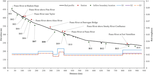
The 2012 open water period has better data quality in terms of the amount of missing values, and thus was used to calibrate the bed roughness, and the 2011 open water period was used for model validation. The bed roughness was calibrated for the three inflow boundary scenarios (S1–S3 in Table 2) separately, and the values used are shown in Fig. 4. The calibrated roughness values are generally in agreement with those used in Trillium Engineering and Hydrographics (1997), which ranged from 0.017 to 0.03 for discharges between 1000 and 10 000 m³/s at the station of Peace River at Fort Vermilion (PRFV), and 0.02 to 0.04 for discharges between 1000 and 5000 m³/s at the station of Peace River at Peace River (PRPR). The calibrated manning’s n values also are overall in line with those calibrated by Huang et al. (2021), which were mainly between 0.01 and 0.03.

Figure 4. Bed profile, bed roughness in three inflow boundary scenarios (S1–S3), inflow boundary and mainstream hydrometric station locations used in the River1D model; the inflow boundaries with larger ungauged sub-basins are indicated in bold.

The simulated results for the two open water periods are shown in Figs 5–8, in comparison with observed water levels and streamflow at five WSC gauge stations. The time series at gauges in the upper reach shows larger fluctuations, which are due to hydropeaking operation from the dam, and this effect attenuates in the downstream direction. In general, the simulated water level and streamflow in all three inflow boundary scenarios show good agreement with the observed data at most stations. For water levels, the values of NS and R² at all stations are over 0.8. The values of NS and R² for streamflow at most stations are greater than 0.8 for the 2011 modelling period; however, for 2012 two of the three scenarios show poor agreement with observed peak flow at the PRFV. Comparing the observed streamflow at the PRPR and PRFV, a reduction by nearly 1700 m³/s of the peak flow occurred over this distance. Such a reduction is not seen in any of the model routed hydrographs no matter which inflow boundary scenario was used. As the magnitude of peak flow is mainly affected by channel roughness (Blackburn and Hicks 2002), the Manning’s n value for the PRPR to PRFV reach (of nearly 450 km) was varied to see the change in the peak flow reduction. It was found that a flow reduction comparable to that observed can only be achieved by increasing the Manning’s n value by over 0.02 for the nearly 450 km reach. Such an increase in roughness caused the water levels at both PRPR and PRFV to increase significantly, resulting in poor agreement with the observed water levels. In addition, the roughness (around 0.04 or higher) is too high compared to the values used in previous studies (e.g. Hicks 1996). It is therefore suspected that the observed flow at PRFV during this period was lower than the actual. This is also supported by the simulation of the 2011 open water flood period. It can be seen from Fig. 6 that the routing of the two flood waves from PRPR to PRFV agrees very well between the modelled and observed.

Figure 5. Comparisons of observed and simulated water level for the 2011 open water period.

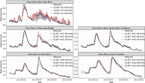
Figure 6. Comparisons of observed and simulated streamflow for the 2011 open water period.

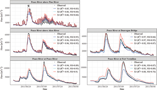
Figure 7. Comparisons of observed and simulated water level for the 2012 open water period.

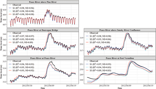
Figure 8. Comparisons of observed and simulated streamflow for the 2012 open water period.

Looking closely at the peak flows, S1, using the multiplication factors from Hicks (1996), significantly underestimated the peak flow at many hydrometric stations, especially during the 2011 open water flood period. For example, the observed largest peak flow at PRPR in 2011 was about 13 630 m³/s, while the simulated value in S1 was only 8966 m³/s. This was likely because flow from large parts of the ungauged sub-basins was not taken into account in S1.

S2 used the modified multiplication factors that account for the streamflow from all the ungauged sub-basins. It significantly improved the open water peak flow simulations at most of the hydrometric stations as compared with S1 (see Figs 6 and 8). However, S2 still evidently underestimated the largest peak flow of the 2011 open water flood event, with the simulated value at PRPR around 10 090 m³/s. This could be due to the underestimation of streamflow in the inflow boundary zones of B07 and B08, located just before PRPR. However, the corresponding largest peak flow at the downstream station of PRFV shows good agreement with the observed. This may indicate that ungauged sub-basin streamflow values in B11 and B12 located between PRPR and PRFV were overestimated. The ungauged area far exceeds the gauged area in B07, B08, B11 and B12 (see Table 2), and thus the runoff production mechanisms for the ungauged sub-basins are probably very different from those of the gauged sub-basins. In this case, the DAR method has large uncertainty and may significantly mis-estimate the ungauged sub-basin streamflow. The uncertainty arising from applying the DAR method to a large ungauged area is small during the 2012 open water period since the streamflow from the large ungauged sub-basins (such as those in B07 and B08) makes a small contribution to the peak flow in non-flood periods.

S3 used SWAT to estimate the ungauged streamflow for the inflow boundary zones containing large ungauged area (B07, B08, B11 and B12). Like S2, S3 overall improved the peak flow at most stations (see Figs 6 and 8). Moreover, S3 provided more reasonable simulation of the largest peak flow at both PRPR and PRFV in 2011, though the simulated value was still a little lower than the observed peak value. However, S3 significantly overestimated the second peak flow at the Peace River at Dunvegan Bridge (PRDB). These results suggest that the SWAT model may have overestimated the ungauged sub-basin streamflow in B07, while somewhat underestimating the streamflow from those ungauged sub-basins between PRDB and PRPR. In addition, S3 overall tends to overestimate during the first peak and low flow periods at PRPR and PRFV. The simulated rising times of the hydrographs and the peaking times were also earlier than the observed. These discrepancies are likely due to uncertainties and/or errors of both observed data and the SWAT model. The geometric data may be another source of uncertainty, as hundreds of kilometres of the study reach used approximated geometry and many of the surveyed cross-sections were obtained in the 1990s.

In general, the comparison of the three inflow boundary scenarios demonstrated that the streamflow from the ungauged sub-basins greatly contributed to the open water flood. The hydrological model is useful in simulating the streamflow in the ungauged area and has a good potential to provide inflow boundaries for the hydraulic model. Nevertheless, the hydrological model needs to be further improved to well capture open water flood.

3.2 River ice breakup periods

Before comparing the modelled results with observed during the breakup periods, it is worth noting that the WSC flow data can contain greater uncertainty when the gauge is affected by ice. WSC uses station-specific open water rating curves to derive flow from continuous measurement of water levels. However, the presence of ice causes the water level–discharge relationship to greatly deviate from the open water rating curve, and the derived flow only represents the maximum possible discharge in the presence of ice. Turcotte and Rainville (2022) explain the procedure that WSC takes to correct the derived discharge. Direct flow measurements provide a good basis for such correction but are only done a couple of times during winter, when the ice cover is safe to work on. When such data are not available, the correction can be subjective. WSC uses the symbol “B” in the discharge data to indicate a gauge station was affected by ice and the discharge was estimated.

Figure 9 shows the retreat of the ice front during the three simulated years, which provides a rough idea of when a gauge station may have not been affected by ice. In the upstream steeper reach where the ice-caused backwater does not extend very far upstream from the ice front, stations Peace River above Pine River, Peace River near Taylor, and Peace River above Alces River were not affected by ice. In the downstream reach where the channel slope is mild, the backwater from ice can extend tens of kilometres upstream depending on the thickness and roughness of the ice cover. The date when the downstream gauge stations like PRDB, Peace River above Smoky River Confluence (PRSRC), PRPR and PRFV were not affected by ice was estimated based on ice front locations, the last “B” symbol in the flow data, and available satellite images of the study reach. The dates when PRDB, PRSRC, PRPR and PRFV were no longer affected by ice were 18 April, 25 April, 26 April and 29 April in 2007; In 2013, these dates were 2 April, 13 April, 15 April, and 7 May. In 2012, PRDB was not affected by ice since the beginning of the simulation while PRSRC, PRPR and PRFV were not affected by ice starting from 16 March, 30 March and 29 April, respectively.

Figure 9. Observed ice front locations of Peace River during the retreating period for 2007, 2012 and 2013.

Figures 10–15 show the simulated water levels and streamflow during the three breakup periods in comparison with the observed. Except PRDB in 2012, the simulated results are all in good agreement with the observations at the stations that were not affected by ice, regardless of the inflow boundary scenario. These are Peace River above Pine River, Peace River above Taylor, and Peace River above Alces River. The simulated water levels at most of the ice-affected stations show favourable agreement with observed, and the water level drop as the ice front passed a gauge station was also well captured. The less satisfactory water level simulations were obtained mainly in three situations: (1) When an ice jam formed or released, as such events are not accounted for in the river ice model. For example, an ice jam formed near PRPR on 21 April 2007 (Alberta Environment Peace River Ice Observation Report No. 52 – 2006/2007), which caused the water level of PRPR to increase by 0.5 to 1 m. The water level peak and late drop after the jam was released was not well simulated by the River1D model (see PRPR in Fig. 10). (2) When the ice front moved a long distance in a relatively short period or the ice front location was not observed for a long time. For example, Fig. 9 shows that in 2007 the ice front moved nearly 100 km near PRPR and PRSRC between 23 and 25 April, and its location was not tracked between 26 and 29 April, during which the ice front moved about 357 km from near PRPR to PRFV. In the former case, the ice breakup was very dynamic and cannot be well represented by a fixed-length transition zone and specified ice velocity. In the latter case, the ice front may have stalled and restarted during the period without ice front location data, and thus linearly interpolating the ice front location between the known data points led to errors in simulating the hydraulic conditions. As a result, the simulated water levels show poor agreement with the observed data at PRSRC, PRPR and PRFV during the above-mentioned time periods. (3) When the ice cover had broken up at a gauge station. The simulated water level was relatively high as compared to the observed values after the ice cover had broken up and the hydraulic conditions near the gauge had returned to near open water conditions. For example, the simulated water levels at PRDB in 2007, and at PRSRC, PRPR, and PRFV in 2012, were all overestimated after the water level dropped significantly. This is likely due to the effect of remnant ice in the river channel. Additionally, the bed roughness may have changed due to ice-caused sediment deposition and scouring, while the bed roughness values calibrated for the open water events were used to simulate the breakup periods.

Figure 10. Comparisons of observed and simulated water level for the 2007 river ice breakup period; the vertical dashed line in a gauge station roughly indicates when the station is not affected by ice.

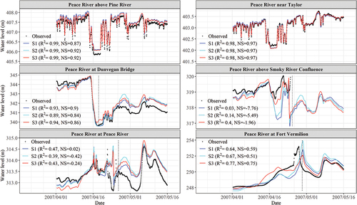
Figure 11. Comparisons of observed and simulated streamflow for the 2007 river ice breakup period; the vertical dashed line in a gauge station roughly indicates when the station is not affected by ice.

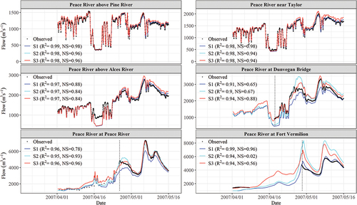
Figure 12. Comparisons of observed and simulated water level for the 2012 river ice breakup period; the vertical dashed line in a gauge station roughly indicates when the station is not affected by ice.

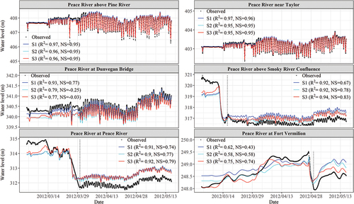
Figure 13. Comparisons of observed and simulated streamflow for the 2012 river ice breakup period; the vertical dashed line in a gauge station roughly indicates when the station is not affected by ice.

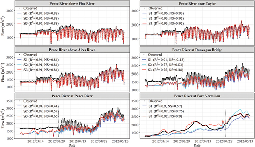
Figure 14. Comparisons of observed and simulated water level for the 2013 river ice breakup period; the vertical dashed line in a gauge station roughly indicates when the station is not affected by ice.

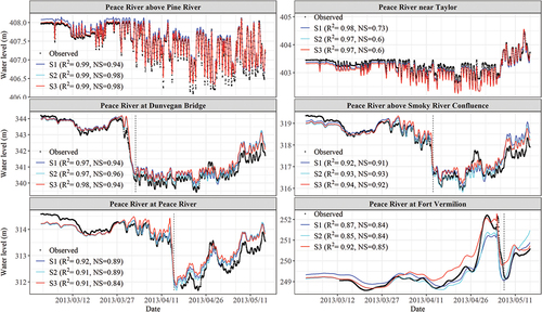
Figure 15. Comparisons of observed and simulated streamflow for the 2013 river ice breakup period; the vertical dashed line in a gauge station roughly indicates when the station is not affected by ice.

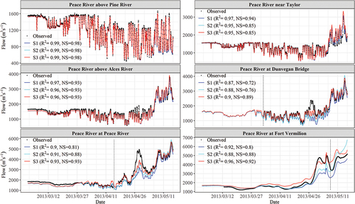
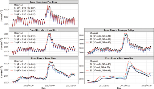
Figures 11, 13 and 15 show the comparison of simulated and observed streamflow during the three breakup periods. The streamflow was well simulated at all the gauge stations that were not affected by ice. The only exception is PRDB in 2012, where the simulated flow with either of the three inflow boundary scenarios was lower than the observed. The simulated streamflow at the PRDB was mainly influenced by inflow from B07, and the spring streamflow was primarily driven by snowmelt. Therefore, data from an SWE station located near B07 were used to assess the accuracy of the simulated SWE. It was found that the SWE values in 2012 were notably lower than in other years. Additionally, the SWE values simulated by the SWAT model were lower than the observed values. As a result, the estimated streamflow from the ungauged sub-basins of the B07 was expected to be lower. This then led to lower simulated streamflow at the PRDB in 2012.

For the ice-affected stations, the inflow boundary scenario S1 again significantly underestimated the peak flow. The only exception is the PRFV flow in 2007, where S1-simulated flow better matched the observed data than the other two scenarios. Based on a satellite image from LANDSAT7 showing the reach ~10 km upstream and downstream of the PRFV, the river was in complete open water on 1 May 2007 18:36:44. However, it was found that after this date, the streamflow at PRFV derived using the station’s open water rating curve and the observed water levels had a much higher peak flow than the WSC published peak flow (7135 m³/s as compared to about 5760 m³/s on 8 May 2007). Therefore, there may be uncertainty and/or error in the published discharge data at PRFV in 2007. This explains the exception identified at PRFV flow in 2007.

S2 improved the peak flow at some stations (e.g. PRPR and PRFV in 2013), but significantly underestimated the snow- and ice-affected peak flows while overestimating the peak flow when river had just turned into open water conditions at many stations (e.g. PRFV in both 2012 and 2013). The runoff production mechanisms and snowfall distribution among various sub-basins may be very different. The DAR method had larger uncertainty in estimating ungauged sub-basin streamflow during snow melting and the river ice breakup period, which then led to poor performance of S2.

S3 generally performed the best of the three inflow boundary scenarios, as it captured the snow- and ice-affected peak flow at most stations very well (e.g. PRDB and PRPR in 2007, PRFV in 2012, and PRFV in 2013). Nevertheless, the discrepancy is still obvious at some stations (e.g. PRPR in 2012), as there may have been some deviations in the inflow boundaries provided by the SWAT model. Moreover, the daily streamflow calculated by the SWAT model was probably not fine enough to capture the very dynamic flood occurring during river ice breakup.

However, the comparison among the three inflow boundary scenarios still demonstrates that the ungauged sub-basins do contribute a large amount of streamflow and can greatly affect the peak flow during snow melting and river ice breakup period. The SWAT model can be a useful tool to provide inflow boundaries for the river ice model during snow melting and river ice breakup period, but the temporal resolution of the output flow of the hydrological model needs to be further improved to better capture floods.

3.3 Streamflow in gauged and ungauged sub-basins

Previous sections demonstrated that the calibrated SWAT model generally performed well in providing inflows for the River1D model. Before the calibrated SWAT model was used to investigate the streamflow contributions of gauged and ungauged sub-basins across the PRB, it was further evaluated by comparing the simulated gauged sub-basin streamflow in the 14 inflow boundary zones with the corresponding observed data (Table 3). Based on the index of multi-year (2004–2013) average annual mean streamflow (MAMS) and annual peak streamflow (MAPS), the streamflow contributions of each inflow boundary zone were roughly quantified. For the observed gauged streamflow, the MAMS index indicates that B01 contributes the most, followed by B09 and B04. However, the most contributing inflow boundary becomes B09 based on the MAPS. This is because B01 is regulated by the dam and its outflow is reduced during flood season. A similar contributing pattern is also seen in SWAT model-simulated results. The relative errors between the observed and simulated gauged sub-basins in each inflow boundary were also computed (Table 3). The absolute values of the relative errors for the first three most contributing inflow boundaries are less than 35%. The larger deviations are often seen in the less contributing inflow boundaries. In general, the calibrated SWAT model has a good performance and can provide reasonable streamflow for both gauged and ungauged sub-basins across the PRB.

Table 3. Summary of the observed and simulated multi-year (2004–2013) average annual mean streamflow (MAMS) and annual peak streamflow (MAPS) for the gauged area in each inflow boundary zone.

Boundary	Station	Gauged area (km^2)	Observed gauged streamflow				SWAT simulated streamflow				Relative error (%)
			MAMS (m^3/s)	Ratio (%)	MAPS (m^3/s)	Ratio (%)	MAMS (m^3/s)	Ratio (%)	MAPS (m^3/s)	Ratio (%)	MAMS	MAPS
B01	07EF001	70 042	1115.8	59.64	1881	23.49	1122.7	55.12	1879.7	26.94	0.62	−0.07
B02	07FA006	9238	64.4	3.44	717.5	8.96	89.2	4.38	726.9	10.42	38.44	1.30
B03	07FB008	1506	11.6	0.62	84.1	1.05	14.2	0.70	218.9	3.14	22.58	160.39
B04	07FB001	11 956	190.3	10.17	1539.3	19.22	182.2	8.95	1003.1	14.38	−4.27	−34.84
B05	07FC001	15 297	45.3	2.42	528.3	6.60	93.1	4.57	448.5	6.43	105.57	−15.10
B06	07FD001	3584	9.9	0.53	167.4	2.09	19.4	0.95	128.1	1.84	95.27	−23.47
B07	07FD009	2840	6.2	0.33	84.5	1.05	11.8	0.58	122.8	1.76	89.82	45.43
B08	07FD006	523	1.6	0.08	36.5	0.46	4.0	0.20	59.6	0.85	153.16	63.14
B09	07GJ001	48 553	327.4	17.50	2242	28.00	401.6	19.72	1848.1	26.49	22.66	−17.57
B10	07HA003	1737	2.6	0.14	46.1	0.58	8.6	0.42	91.1	1.31	227.27	97.51
B11	07HC001	4637	10.9	0.58	158.2	1.98	8.0	0.39	29.2	0.42	−26.70	−81.52
B12	07HF002	736	2.7	0.14	29.4	0.37	1.0	0.05	9.9	0.14	−61.57	−66.21
B13	07JF003	2370	15.6	0.83	104.8	1.31	11.3	0.55	112.5	1.61	−27.80	7.35
B14	07JD002	33 044	66.7	3.57	388.3	4.85	69.8	3.43	298.7	4.28	4.62	−23.07

The ratio indicates the percentage of MAMS and MAPS of each boundary gauged area relative to those of the total gauged area; ratio values over 5% are in bold to highlight the stations contributing more; the relative error is computed from the simulated and observed MAMS and MAPS.

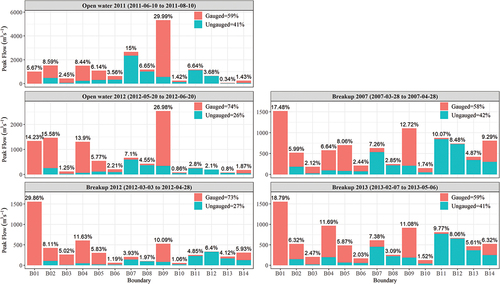
The contribution from the gauged and ungauged sub-basins to the peak flow during the simulated open water and river ice breakup periods is shown in Fig. 16. It is important to note that near the end of each simulated river ice breakup period, the river had returned to open water condition, and these open water periods were excluded when determining the peak flow during river breakup. For the non-flood periods, such as the 2012 open water and breakup periods, the ungauged sub-basins contributed about 26% and 27% of the peak flow, respectively. This is nearly the same as the percentage area of the ungauged sub-basins relative to the whole modelled area, which is ~26.5%. However, the ungauged sub-basins contributed 41% to 42% of the peak flow for the 2011 flood period and the mechanical river ice breakup periods (i.e. 2007 and 2013). The inflow boundary zones for which the ungauged area far exceeds the gauged area, such as B07, B08, B11 and B12, contributed a large amount of streamflow for the open water and breakup flood years. Given that the peak flow simulated by S3 during river ice breakup was still underestimated, the ungauged sub-basins could have contributed more to the peak flow. This emphasizes the importance of considering the ungauged sub-basin streamflow when setting up a river ice model or hydraulic model.

Figure 16. Peak flow contributions of gauged and ungauged sub-basins in various inflow boundary zones; the values on top of each column show percentage of peak flow contribution from each inflow boundary zone.

4 Conclusions and recommendations

This study constructed a hydrological and river ice modelling framework with SWAT and River1D to investigate the impact of the streamflow from ungauged sub-basins on peak flows during open water and river ice breakup periods in the Peace River Basin (PRB). In the framework, the DAR method and the hydrological model were employed to estimate the ungauged sub-basin streamflow within the PRB and improve the inflow boundaries for the River1D model. Comparing to the simple DAR method, it was shown that the hydrological model can provide more accurate estimation of the ungauged sub-basin streamflow for regions with large ungauged sub-basin area during flood events. In particular, the SWAT model outperformed the DAR method for simulating the ungauged streamflow during river ice breakup periods, mainly because the SWAT model can reasonably simulate snow-affected streamflow. However, it is important to acknowledge that certain discrepancies may still arise due to the uncertainties inherent in the observed data and model structures. For instance, a uniform SWE was assumed for each sub-basin in the SWAT model. The uncertainty and error within the SWAT model can potentially propagate into the River1D model by providing inflow boundaries for River1D. Nevertheless, the proposed modelling framework employs an iterative calibration process between the river ice model and the hydrological model, which helps to mitigate the potential error propagation between the models. In general, both the DAR method and the hydrological model can provide significantly improved inflow boundaries to the River1D model, which can then better capture the peak flow. Meanwhile, the River1D simulation results demonstrated that the streamflow from the ungauged sub-basins of the PRB can greatly affect the peak flow simulation of the river ice model for both open water and river ice breakup flood events. Based on the simulated streamflow from the SWAT model, it was found that the ungauged sub-basins can contribute nearly half of the peak flow for the open water and river ice breakup flood events even though they account for only about 26.5% of the whole study area. Overall, the findings in this study can contribute to open water and river ice breakup flood simulation, and water resources planning and management in the PRB. The proposed methods also can provide insights for researchers on modelling flood events in other ungauged or partially ungauged basins.

The hydrological and river ice modelling framework can be a useful tool to forecast snow- and ice-related flood events. The hydrological model can provide necessary inflow boundaries for the river ice model, while the channel routing method used in the river ice model also can better simulate the ice-affected streamflow. In this study, ice breakup was only considered in the mainstream of the Peace River. In future work, the effects of river ice breakup on streamflow should be considered in the whole Peace River network, through deeply coupling the physics-based river ice models with hydrological models to better simulate snow- and ice-affected spring streamflow. The SWAT model developed in this study only provided daily streamflow, which would need to be refined to capture more dynamic flood events such as those associated with mechanical breakup, especially in large cold-region watersheds. Calibrating a sub-daily hydrological model in a large river basin can be computationally expensive and time consuming. Therefore, more efforts should also be devoted to improving the efficiency of hydrological model calibration. Furthermore, the uncertainties in the observed streamflow data due to ice effects will need to be further assessed to better calibrate and validate the modelling framework. In some cases, hydrological model results can be used in correcting streamflow observations influenced by ice (Dahl et al. 2019), but the performance needs to be further improved as the hydrological model cannot accurately account for the ice effects.

The hydrological and river ice modelling framework proposed in this study has good potential to effectively correct observations affected by ice and reconstruct winter flow data because it can take into account of the impacts of snow and ice on streamflow. Nevertheless, its performance needs to be assessed in future study. In addition, it would be beneficial and imperative to implement deeper coupling of the hydrological and river ice models in future study, i.e. solving the equations governing the hydrological, hydraulic and river ice processes simultaneously. The deeply integrated coupling has the potential to provide a more accurate representation of the interactions among the various concurrent processes, and thereby create a more efficient and effective modelling system and enhance the overall performance. The challenges of this approach are model complexity, computational demand, data requirements, calibration, and parameterization.

Disclosure statement

No potential conflict of interest was reported by the authors.

Additional information

Funding

The work was funded by the Natural Science and Engineering Research Council of Canada (NSERC) Discovery Grants programme [RGPIN-2021-02887].

References

- Abbaspour, K.C., 2015. SWAT calibration and uncertainty programs—A user manual. In: Eawag is the Swiss Federal Institute of Aquatic Science and Technology. Eawag, Switz.
- Andrishak, R. and Hicks, F., 2008. Simulating the effects of climate change on the ice regime of the Peace River. The Canadian Journal of Civil Engineering, 35 (5), 461–472. doi:10.1139/L07-129.
- Arnold, J.G., et al., 1998. Large area hydrologic modeling and assesment part I: model development. The Journal of the American Water Resources Association (JAWRA), 34 (1), 73–89. doi:10.1111/j.1752-1688.1998.tb05961.x.
- Asquith, W.H., Roussel, M.C., and Vrabel, J., 2006. Statewide analysis of the drainage-area ratio method for 34 streamflow percentile ranges in Texas. Reston, VA: US Geological Survey.
- Beltaos, S., 2008. Progress in the study and management of river ice jams. Cold Regions Science and Technology, 51 (1), 2–19. doi:10.1016/j.coldregions.2007.09.001.
- Beltaos, S. and Prowse, T., 2009. River‐ice hydrology in a shrinking cryosphere. Hydrological Processes, 23 (1), 122–144. doi:10.1002/hyp.7165.
- Beltaos, S. and Prowse, T.D., 2001. Climate impacts on extreme ice-jam events in Canadian rivers. Hydrological Sciences Journal, 46 (1), 157–181. doi:10.1080/02626660109492807.
- Blackburn, J. and Hicks, F., 2002. Combined flood routing and flood level forecasting. The Canadian Journal of Civil Engineering, 29 (1), 64–75. doi:10.1139/l01-079.
- Blackburn, J. and She, Y., 2019. A comprehensive public-domain river ice process model and its application to a complex natural river. Cold Regions Science and Technology, 163 (April), 44–58. doi:10.1016/j.coldregions.2019.04.010.
- Blöschl, G. and Sivapalan, M., 1995. Scale issues in hydrological modelling: a review. Hydrological Processes, 9 (3–4), 251–290. doi:10.1002/hyp.3360090305.
- Bonnifait, L., et al., 2009. Distributed hydrologic and hydraulic modelling with radar rainfall input: reconstruction of the 8-9 September 2002 catastrophic flood event in the Gard region, France. Advances in Water Resources, 32 (7), 1077–1089. doi:10.1016/j.advwatres.2009.03.007.
- Booker, D.J. and Woods, R.A., 2014. Comparing and combining physically-based and empirically-based approaches for estimating the hydrology of ungauged catchments. Journal of Hydrology, 508, 227–239. doi:10.1016/j.jhydrol.2013.11.007.
- Burrell, B.C., Beltaos, S., and Turcotte, B., 2021. Effects of climate change on River-Ice processes and ice jams. International Journal of River Basin Management, 21, 1–78. doi:10.1080/15715124.2021.2007936.
- Chen, F., Shen, H.T., and Jayasundara, N., 2006. A one-dimensional comprehensive river ice model. In: Proceedings of the 18th IAHR International Symposium on Ice. Sapporo, Japan: Citeseer.
- Chen, Y., et al., 2023. Evaluation and uncertainty assessment of weather data and model calibration on daily streamflow simulation in a large-scale regulated and snow-dominated river basin. Journal of Hydrology, 617, 129103. doi:10.1016/j.jhydrol.2023.129103
- Dahl, M.-P.J., et al., 2019. Variation in discharge data and correction routines at the Norwegian Water resources and energy directorate, Norway. In: CGU HS Committee on River Ice Process and the Environment 20h Work Hydraulic Ice Cover. Rivers Ottawa, Ontario, Canada.
- Das, A., Rokaya, P., and Lindenschmidt, K.E., 2020. Ice-Jam flood risk assessment and hazard mapping under future climate. Journal of Water Resources Planning and Management, 146 (6), 1–12. doi:10.1061/(ASCE)WR.1943-5452.0001178.
- De Rham, L., et al., 2020. A Canadian River Ice database from the national hydrometric program archives. Earth System Science Data (ESSD), 12 (3), 1835–1860. doi:10.5194/essd-12-1835-2020.
- Dessie, M., et al., 2015. Water balance of a lake with floodplain buffering: lake Tana, Blue Nile Basin, Ethiopia. Journal of Hydrology, 522, 174–186. doi:10.1016/j.jhydrol.2014.12.049.
- Emerson, D.G., Vecchia, A.V., and Dahl, A.L., 2005. Evaluation of drainage-area ratio method used to estimate streamflow for the Red River of the North Basin, North Dakota and Minnesota. Reston, VA: US Department of the Interior, US Geological Survey.
- Ergen, K. and Kentel, E., 2016. An integrated map correlation method and multiple-source sites drainage-area ratio method for estimating streamflows at ungauged catchments: a case study of the Western Black Sea Region, Turkey. Journal of Environmental Management, 166, 309–320. doi:10.1016/j.jenvman.2015.10.036.
- French, H.M., 2017. The periglacial environment. Hoboken, NJ: John Wiley & Sons.
- Gianfagna, C.C., et al., 2015. Watershed area ratio accurately predicts daily streamflow in nested catchments in the Catskills, New York. Journal of Hydrology: Regional Studies, 4, 583–594. The Authors. doi:10.1016/j.ejrh.2015.09.002.
- Grimaldi, S., et al., 2019. Challenges, opportunities, and pitfalls for global coupled hydrologic-hydraulic modeling of floods. Water Resources Research, 55 (7), 5277–5300. doi:10.1029/2018WR024289.
- Guo, Y., et al., 2021. Regionalization of hydrological modeling for predicting streamflow in ungauged catchments: a comprehensive review. Wiley Interdisciplinary Reviews: Water, 8 (1), e1487. doi:10.1002/wat2.1487.
- He, Y., Bárdossy, A., and Zehe, E., 2011. A review of regionalisation for continuous streamflow simulation. Hydrology and Earth System Sciences, 15 (11), 3539–3553. doi:10.5194/hess-15-3539-2011.
- Hersbach, H., et al., 2020. The ERA5 global reanalysis. Quarterly Journal of the Royal Meteorological Society, 146 (730), 1999–2049. doi:10.1002/qj.3803.
- Hicks, F., 1996. Hydraulic flood routing with minimal channel data: peace River, Canada. The Canadian Journal of Civil Engineering, 23 (2), 524–535. doi:10.1139/l96-057.
- Hicks, F. and Steffler, P.M., 1990. Finite element modeling of open channel flow. Department of civil engineering, University of Alberta, Edmonton, Alta. Water Resources Engineering Reports, (90–6).
- Hicks, F. and Steffler, P.M., 1992. Characteristic dissipative Galerkin scheme for open-channel flow. Journal of Hydraulic Engineering, 118 (2), 337–352. doi:10.1061/(ASCE)0733-9429(1992)118:2(337).
- Hrachowitz, M., et al., 2013. A decade of Predictions in Ungauged Basins (PUB)-a review. Hydrological Sciences Journal, 58 (6), 1198–1255. doi:10.1080/02626667.2013.803183.
- Huang, F., Jasek, M., and Shen, H.T. (2021) Simulation of the 2014 dynamic ice breakup on the Peace River 1–19.
- Krause, P., Boyle, D.P., and Bäse, F., 2005. Comparison of different efficiency criteria for hydrological model assessment. Advances in Geosciences, 5, 89–97. doi:10.5194/adgeo-5-89-2005
- Li, Q., et al., 2019a. A combined method for estimating continuous runoff by parameter transfer and drainage area ratio method in ungauged catchments. Water, 11 (5), 1104. doi:10.3390/w11051104.
- Li, W., et al., 2019b. Risk assessment and sensitivity analysis of flash floods in ungauged basins using coupled hydrologic and hydrodynamic models. Journal of Hydrology, 572 (February), 108–120. doi:10.1016/j.jhydrol.2019.03.002.
- Lindenschmidt, K.E., 2017. RIVICE-A non-proprietary, open-source, one-dimensional river-ice model. Water (Switzerland), 9 (5). doi:10.3390/w9050314.
- Lindenschmidt, K.E., et al., 2019. A novel stochastic modelling approach for operational real-time ice-jam flood forecasting. Journal of Hydrology, 575 (June 2018), 381–394. doi:10.1016/j.jhydrol.2019.05.048.
- Liu, G., et al., 2015. Discharge and water‐depth estimates for ungauged rivers: combining hydrologic, hydraulic, and inverse modeling with stage and water‐area measurements from satellites. Water Resources Research, 51 (8), 6017–6035. doi:10.1002/2015WR016971.
- Liu, L., Li, H., and Shen, H.T., 2006. A two-dimensional comprehensive river ice model. In: Proceedings of the 18th IAHR International Symposium on Ice, Sapporo, Japan, 69–76.
- McCuen, R.H. and Levy, B.S., 2000. Evaluation of peak discharge transposition. Journal of Hydrologic Engineering, 5 (3), 278–289. doi:10.1061/(ASCE)1084-0699(2000)5:3(278).
- Merz, B., et al., 2021. Causes, impacts and patterns of disastrous river floods. Nature Reviews Earth & Environment, 2 (9), 592–609. doi:10.1038/s43017-021-00195-3.
- Mishra, A., et al., 2022. An overview of flood concepts, challenges, and future directions. Journal of Hydrologic Engineering, 27 (6), 1–30. doi:10.1061/(asce)he.1943-5584.0002164.
- Mishra, A.K. and Coulibaly, P., 2009. Developments in hydrometric network design: a review. Reviews of Geophysics, 47 (2). doi:10.1029/2007RG000243.
- Moriasi, D.N., et al., 2007. Model evaluation guidelines for systematic quantification of accuracy in watershed simulations. Transactions of the ASABE, 50 (3), 885–900. doi:10.13031/2013.23153.
- Neitsch, S., et al., 2011. Soil & water assessment tool theoretical documentation version 2009. Texas Water Resources Institute, 1–647. doi:10.1016/j.scitotenv.2015.11.063.
- Nguyen, P., et al., 2016. A high resolution coupled hydrologic–hydraulic model (HiResFlood-UCI) for flash flood modeling. Journal of Hydrology, 541, 401–420. doi:10.1016/j.jhydrol.2015.10.047.
- Pagliero, L., et al., 2019. Investigating regionalization techniques for large-scale hydrological modelling. Journal of Hydrology, 570 (December 2018), 220–235. doi:10.1016/j.jhydrol.2018.12.071.
- Parajka, J., et al., 2013. Comparative assessment of predictions in ungauged basins-part 1: runoff-hydrograph studies. Hydrology and Earth System Sciences, 17 (5), 1783–1795. doi:10.5194/hess-17-1783-2013.
- Razavi, T. and Coulibaly, P., 2013. Streamflow prediction in ungauged basins: review of regionalization methods. Journal of Hydrologic Engineering, 18 (8), 958–975. doi:10.1061/(asce)he.1943-5584.0000690.
- Salinas, J.L., et al., 2013. Comparative assessment of predictions in ungauged basins-part 2: flood and low flow studies. Hydrology and Earth System Sciences, 17 (7), 2637–2652. doi:10.5194/hess-17-2637-2013.
- She, Y., et al., 2009. Athabasca River ice jam formation and release events in 2006 and 2007. Cold Regions Science and Technology, 55 (2), 249–261. Elsevier B.V. doi:10.1016/j.coldregions.2008.02.004.
- She, Y. and Hicks, F., 2006. Modeling ice jam release waves with consideration for ice effects. Cold Regions Science and Technology, 45 (3), 137–147. doi:10.1016/j.coldregions.2006.05.004.
- Singh, L., et al., 2022. Streamflow regionalisation of an ungauged catchment with machine learning approaches. Hydrological Sciences Journal, 67 (6), 886–897. doi:10.1080/02626667.2022.2049271.
- Sivapalan, M., 2003. Prediction in ungauged basins: a grand challenge for theoretical hydrology. Hydrological Processes, 17 (15), 3163–3170. doi:10.1002/hyp.5155.
- Sivapalan, M., et al., 2003. IAHS decade on Predictions in Ungauged Basins (PUB), 2003-2012: shaping an exciting future for the hydrological sciences. Hydrological Sciences Journal, 48 (6), 857–880. doi:10.1623/hysj.48.6.857.51421.
- Taggart, J., 1995. The Peace River natural flow and regulated flow scenarios-daily flow data report. In: Surface Water Assessment Branch, Alberta Environmental Protection. Edmonton, AB.
- Tellman, B., et al., 2021. Satellite imaging reveals increased proportion of population exposed to floods. Nature, 596 (7870), 80–86. doi:10.1038/s41586-021-03695-w.
- Thériault, I., Saucet, J.-P., and Taha, W., 2010. Validation of the Mike-Ice model simulating river flows in presence of ice and forecast of changes to the ice regime of the Romaine river due to hydroelectric project. In: Proceedings of the 20th IAHR International Symposium on Ice. Lahti, Finland, 14–17.
- Timalsina, N.P., Alfredsen, K.T., and Killingtveit, Å., 2015. Impact of climate change on ice regime in a river regulated for hydropower 1. The Canadian Journal of Civil Engineering, 42 (9), 634–644. doi:10.1139/cjce-2014-0261.
- Trillium Engineering and Hydrographics, 1997. Ice formation and breakup at the town of Peace River: a study of regulated conditions, 1969–94. Edmonton, Alta: Trillium Engineering and Hydrographics Inc., Report No. 380.
- Turcotte, B., Burrell, B.C., and Beltaos, S., 2019. The impact of climate change on breakup ice jams in Canada : state of knowledge and research approaches.
- Turcotte, B. and Rainville, F., 2022. A new winter discharge estimation procedure: Yukon proof of concept. In: 26th IAHR Int. Symp. Ice, Montréal, Canada.
- Viglione, A., et al., 2013. Comparative assessment of predictions in ungauged basins - part 3: runoff signatures in Austria. Hydrology and Earth System Sciences, 17 (6), 2263–2279. doi:10.5194/hess-17-2263-2013.
- Winchell, M., et al., 2013. ArcSWAT interface for SWAT2012: user’s guide. In: Blackland Research Center, Texas AgriLife Research. College Station, 1–464.
- Ye, Y. and She, Y., 2021. A systematic evaluation of criteria for river ice breakup initiation using River1D model and field data. Cold Regions Science and Technology, 189 (May), 103316. doi:10.1016/j.coldregions.2021.103316.
- Zelelew, M.B. and Alfredsen, K., 2014. Use of cokriging and map correlation to study hydrological response patterns and select reference stream gauges for ungauged catchments. Journal of Hydrologic Engineering, 19 (2), 388–406. doi:10.1061/(asce)he.1943-5584.0000803.
- Zhang, L., et al., 2017. Stream flow simulation and verification in ungauged zones by coupling hydrological and hydrodynamic models: a case study of the Poyang Lake ungauged zone. Hydrology and Earth System Sciences, 21 (11), 5847–5861. doi:10.5194/hess-21-5847-2017.
- Zhang, Y. and Chiew, F.H.S., 2009. Relative merits of different methods for runoff predictions in ungauged catchments. Water Resources Research, 45 (7). doi:10.1029/2008WR007504.