Estimation of the time of concentration of small watersheds located in northeastern North America

Abstract

The time of concentration is an important concept in hydrology. It provides a characteristic hydrological response time (CHRT) useful in many applications. Estimation of the time of concentration is challenging because small watersheds (< 100 km²) with subdaily flow and precipitation records are uncommon. Many practitioners therefore use empirical equations developed from watersheds exposed to various climate and with different attributes. The main objective of this study is to develop an approach to estimate the CHRT from physiographic characteristics for small watersheds located in Ontario, Quebec and the northeastern USA. Regression trees are used to identify the physiographic characteristics associated with CHRT. The fraction of lakes and wetlands was identified as the most significant attribute related to CHRT, followed by the ratio between the main watercourse length and the square root of the main watercourse slope. Uncertainties on estimated CHRT values based on regression tree are also provided.

Keywords:

• time of concentration
• time to peak
• small watersheds
• rational method
• regression tree
• lakes and wetlands

Disclaimer

As a service to authors and researchers we are providing this version of an accepted manuscript (AM). Copyediting, typesetting, and review of the resulting proofs will be undertaken on this manuscript before final publication of the Version of Record (VoR). During production and pre-press, errors may be discovered which could affect the content, and all legal disclaimers that apply to the journal relate to these versions also.

1. Introduction

The time of concentration is a key concept in hydrology as it provides a timescale for the hydrological response useful to estimate maximum peak flows of given return period (Michailidi et al. 2018). It is often defined as the time for a particle of water to travel from the hydrologically most distant point to the watershed outlet (Mulvany, 1851; McCuen, 2009). Although the theoretical definition may seem obvious and easy to understand, the ‘operational’ definition remains challenging and can lead to a misunderstanding of hydrological processes (Beven, 2020).

Incidentally, there is a lot of confusion around the concept and the definition of the time of concentration. A brief survey on that topic reveals an astonishing diversity of definitions (McCuen, 2009) and approaches to estimate its value from flow and precipitation series (Singh, 1988). There is also an unclear distinction with some other hydrological timescales such as the ‘time of rise’ (Espey et al. 1966), ‘time to peak’ (McCuen et al. 1984), ‘lag time’ (McCuen, 2009), and ‘time to equilibrium’ (Beven, 2020), as they are often used interchangeably.

Nevertheless, the estimation of a characteristic hydrological response time (CHRT; Bell and Karr, 1969), for an ungauged watershed remain essential, for example for the application of the rational method still widely used by the engineering community (Dhakal et al., 2013; Grimaldi and Petroselli, 2015). Numerous empirical equations estimating the CHRT from watershed physiographic characteristics have been proposed in the literature and are still widely applied. It should be noted that the expression characteristic hydrological response time, or CHRT, will be used hereafter to refer to what is usually called the time of concentration.

Hydrological response depends on rainfall event characteristics, the physiographic characteristics, and initial state of the watershed (Singh, 1997; Paschalis et al. 2014). In that sense, the CHRT may be viewed as an ‘average’ response time over various rainfall conditions and initial hydrological conditions of the watershed, which can be related to the physiographic characteristics of the watershed. Many empirical equations have been proposed over the years to estimate CHRT from watershed characteristics (for a review see Gericke and Smithers, 2014). In some cases, no or little information on the watersheds used to develop these equations is available (Grimaldi et al. 2012). It is therefore difficult to assess the ‘transferability’ of these empirical equations to other watersheds. Another problematic aspect is that, for many empirical equations, no information about the characteristics of the hydrographs used to develop these equations is available (Williams, 1922; FAA, 1970). For some other equations, like the one proposed by Kirpich (1940), only two years of flow records were used to develop the equation (Ramser, 1927). Serious doubts can therefore be raised on the reliability of these equations to estimate CHRT for peak flow associated with large return period event.

Empirical equations have been proposed for small to very small watersheds, usually those where the rational method is applied (Gericke and Smithers, 2016b). However, these watersheds often have very similar physiographic characteristics and land use. For example, all the watersheds considered by Kirpich (1940), Espey et al. (1966), Folmar and Miller (2008), and Michaud et al. (2014) are mainly agricultural. All the watersheds used in Sheridan (1994) are similar both in terms of land use and mean slope, mainstream slope, and drainage density.

Nevertheless, in the absence of any valuable information, practitioners sometimes apply these equations to watersheds that may be very different from the watersheds used to develop these equations or apply them to watersheds exposed to very different climatic conditions (McCuen et al. 1984; Gericke and Smithers, 2014; Gericke and Smithers, 2016a). In Sweden, the equation of Miller, developed in 1951 in Australia is used with the rational method (Gericke and Smithers, 2014). In South Africa, the Kerby’ equation (Kerby, 1959) and the United States Bureau of Reclamation’s equation (USBR, 1973) are used, both equations being developed in United States (Gericke and Smithers, 2014). Incidentally, 30 of the 39 equations listed in Gericke and Smithers (2014) were developed from watersheds located in USA. Canada is no exception since the Williams’ equation (Williams, 1922), developed in India, and the Airport’s equation (FAA, 1970) developed in United States, are used in Ontario and Québec (MTO, 1997; Transport Québec, 2017).

Many authors have questioned the reliability of commonly used empirical equations after comparison with observed datasets (Grimaldi et al. 2012; Gericke and Smithers, 2016a, Ravazzani et al. 2019). Similar analyses were done back in the 80ʹs and 90ʹs (see e.g., McCuen et al. 1984; Hotchkiss and McCallum 1995). The technical and financial risk associated with the use of possibly inaccurate empirical equations may be huge (McCuen, 2009; Gericke and Smithers, 2016a). It is therefore crucial to develop empirical equations based on local dataset, but it remains challenging considering that very few small watersheds are monitored, and available flow records are often short.

The main objective of this paper is to develop an approach to estimate the CHRT for small watersheds (<100 km²) located in eastern Canada and in northeastern United States. Data from 93 watersheds with various physiographic characteristics were compiled. CHRT at these watersheds were estimated from flow records. Comparisons with existing empirical equations are also tested. Finally, an approach to estimate CHRT from physiographic characteristics, based on regression tree, is proposed and uncertainties on these values are provided.

2. Selected watersheds

A total of 93 watersheds smaller than 100 km² with subdaily flow series (15-min time step) located in Canada (Ontario and Quebec) and the northeastern USA (Maine Vermont, New York, and Massachusetts) is considered in this study (Table 1 and Figure 1). These watersheds range from 0.6 to 100 km² and half of them are less than 40 km² (Figure 2). Small watersheds were selected since estimated CHRT are intended to be used as an input to the rational method, which is adapted to small watersheds, where it is assumed that precipitation is uniformly distributed over the watershed (Rossmiller, 1980). Application of the rational method to large watersheds may indeed result in overestimated peak flows (Pilgrim and Cordery, 1993). The maximum area of 100 km² is based on studies from Young et al. (2009), and Young and McEnroe (2014). No control structure is present on these watersheds.

Table 1. Watershed locations with organizations responsible of operating the hydrometric stations, and number of watersheds under their responsibility.

Province/State	Organization	Number of watersheds
Quebec	MELCCFP^1	11
	IRDA^2	3
Ontario	ECCC^3	37
Maine (ME)	USGS^4	4
Massachussetts (MA)		5
New York (NY)		27
Vermont (VT)		6
Total		93

1 - Ministère de l’environnement et de la lutte contre les changements climatiques, de la Faune et des Parcs

2 - Institut de recherche et de développement en Agroenvironnement

3 - Environment and Climate Change Canada

4 - United States Geological Survey

Figure 1. Map locating the 93 watersheds under study.

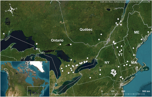
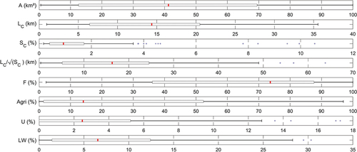
Figure 2. Box plots of the main physiographic characteristics of the 93 watersheds under study. Red bar defines the median value while the rectangles delineate the 1^st (Q1) and 3^rd (Q3) quartiles. Whiskers correspond to 1.5 times the interquartile range (Q3 - Q1), and + to values above 1.5 times the interquartile range. A: watershed area (km²); L_C: main watercourse length (km); S_C: main watercourse slope (%); ${\text{L}}_{\text{C}}/\sqrt{{\text{S}}_{\text{C}}}$: ratio between the main watercourse length and the square root of the main watercourse slope (km); F: forest (%); Agri: agriculture (%); U: urban (%); LW: lake and wetland (%).

Each watershed has at least 10 valid years of recorded flow. A valid year is defined as a year with less than 20% missing 15-min records over the period from June 1^st to October 31^st. This period is considered since flows recorded before June 1^st or after October 31^st may be influenced by snowmelt or ice cover, particularly for watersheds located in the northern part of the study area. Measured flows may as well be unreliable due to the presence of ice (Dibike et al. 2021). The 20% threshold for missing data was selected to maximize the probability to capture the actual annual maxima flows of the June 1st to October 31st period and while keeping a maximum of years and stations despite the presence of many years with missing data. On average, 21 valid years are available with eight watersheds having more than 40 valid years. Finally, annual maxima flow (June to October period) series were extracted at each station, and stationarity of these series was assessed through the Mann-Kendall test. No significant trend was detected at the 95% confidence level.

Physiographic characteristics listed in Table 2 were estimated for all 93 watersheds. Figure 2 presents the distributions of eight of these physiographic characteristics. Median watersheds area is 42 km² and half the watersheds have areas between 13 km² and 69 km². Half of the watersheds are covered by forest over more that 74 % of their surface. Those with smaller forest cover are mostly agricultural. Lakes and wetlands (LW) are present in almost all catchments (89 out of 93) but cover less than 5 % of the area for 39 watersheds. A majority of watersheds (55) have LW covers ranging from 5% to 20%, and only five catchments have LW covering more than 20%. Urban areas are marginal (median of 6%) and no watershed have more than 17% of urban areas.

Table 2. Physiographic characteristics considered in this study.

Characteristic (units)	Symbol/equation
Area (km^2)	A
Mean watershed slope (%)	${\text{S}}_{\text{B}}$
Main watercourse length (km)	${\text{L}}_{\text{C}}$
Main watercourse slope (%)	${\text{S}}_{\text{C}}$
${\text{L}}_{\text{C}}/\sqrt{{\text{S}}_{\text{C}}}$ (km)	${\text{L}}_{\text{C}}/\sqrt{{\text{S}}_{\text{C}}}$
Total hydrographic network length (km)	${\text{L}}_{\text{HN}}$
Drainage density (km/km^2)	DD (${\text{L}}_{\text{HN}}/\text{A})$
Width (km)	W ($\text{A}/{\text{L}}_{\text{C}}$)
Land use^A (%)	Forest (F), cropland, grassland, agriculture (cropland + grassland) (Agri), urban (U), lake, wetland, and lake + wetland (LW)
Hydrologic soil category^B (%)	AB and CD
Connectivity between LW and hydrographic network^C (%)	C
Hydrographic network separation^D (%)	${\text{S}}_{\text{HN}}$
Lakes and wetlands localisation within watershed^E (%)	Downstream, Center, Upstream

A. Québec and Ontario: Annual crop inventory from Agriculture and agri-food Canada (year 2016; https://open.canada.ca/data/en/dataset/ba2645d5-4458-414d-b196-6303ac06c1c9; USA: National Land Cover Database (year 2011; https://www.mrlc.gov/data/nlcd-2011-land-cover-conus)

B. Québec: Gagné et al. (2013) and Mailhot et al. (2018); Ontario: Soil survey complex (https://data.ontario.ca/dataset/soil-survey); USA: SSURGO - Soil hydrologic group ()

C. Percentage of the main hydrographic network that go through LW.

D. Ratio between the area of the watersheds located at a certain distance from the outlet and the total area of the watershed. A small ratio at a point close to the outlet implies that two distinct sub-watersheds may influenced the CHRT of the watershed.

E. The watershed is divided into three sub-watersheds with outlet at 0.25 and 0.50 along the main watercourse from the outlet (Mailhot et al., 2021). The fraction of LW in each sub-watershed is estimated and the sub-watershed with the largest fraction is used to determine LW localisation.

3. Methodology

3.1 Definition and estimation of the characteristic hydrological response time

The operational definition of the CHRT used in this study is the one first proposed by Ramser (1927): “the time needed for the flow to change from the lowest stage to the highest stage”. This definition is commonly referred as the time of rise (Espey et al., 1966; Hotchkiss and McCallum, 1995), which was more recently referred as the time to peak (T_P; McCuen et al., 1984; Gericke and Smithers, 2014). Based on that definition, two specific time variables (see the terminology proposed by McCuen, 2009) of the hydrograph must be estimated (Figure 3), the starting time of direct runoff (t₁), and the time of occurrence of the peak discharge or peak flow (t₂).

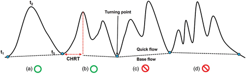
Figure 3. Four types of hydrographs considered in this study: A) single peak hydrograph; B) two-peak hydrograph with first peak larger than the second one; C) two-peak hydrograph with second peak larger than the first one; D) multiple-peak (more than two peaks) hydrograph. t₁ corresponds to the starting time of the hydrograph, t₃ to the ending time, t₂ to the time of occurrence of the peak flow. CHRT is associated with time to peak (t₂ - t₁).

The time to peak is the only definition of the CHRT requiring only flow series. The other definitions proposed in the literature request time variables of the hyetograph associated to the hydrograph (Singh, 1988). In our case, very few stations recording subdaily (e.g., hourly) rainfall series covering the same period as the flow series and located within or close to each watershed are available, since small watersheds are considered. High density networks would be needed to correctly assess the spatial and temporal variability of subdaily rainfalls (Michelon et al., 2021). Furthermore, spatial and temporal resolutions of available gridded rainfall datasets are still too coarse to adequately reproduce local subdaily rainfall series (Newman et al., 2019).

3.2 Hydrograph separation method

The Smoothed Minima Baseflow Separation (SMBS) method, first described in Institute of Hydrology (1980), was used to extract the hydrographs from the observed flow records. The method is based on the identification of ‘turning points’, which corresponds to transition to and from base flow conditions (Figure 3). These turning points are used to separate the baseflow from the runoff and extract hydrographs. This method is simple to implement and provides reproducible results.

SMBS was selected instead of other baseflow or baseflow index methods (Nathan and McMahon, 1990; Xie et al., 2020). Tarasova et al. (2018) comparing five different methods for event separation, including SMBS, which they called nonparametric simple smoothing method, concluded that, despite its simplicity, SMBS enables the unambiguous identification of the beginning points of hydrograph for a wide range of watersheds. In that context, SMBS provides realistic results and is consistent with the beginning of hydrograph identified through visual inspection. Since the SMBS was not originally developed and applied to small watersheds with subdaily flow records, many modifications have been made to the original method to adapt it (see Supplementary material).

The modified SMBS method has been applied to each watershed. Since hydraulic design deals with extreme flow conditions, the most extreme peak flows at each watershed were retained for an average of 2.5 peaks flows per year, and corresponding hydrographs were extracted. These hydrographs were then classified into four types according to the number of peak flows and their relative amplitudes (Figure 3). Single and two-peak hydrographs with largest peak occurring first were retained for further analysis (hydrographs A and B of Figure 3 respectively). These two types of hydrographs were selected because the time to peak in these cases may be assumed adequately related to the CHRT. An analysis has been carried out to see if major peak flows were rejected when considering only A and B hydrographs. It shows that the highest peak flow ever recorded at each station is associated with type A or B hydrographs at 75% of the watersheds. Type A and B hydrographs remain the dominant hydrograph type up to the tenth highest peak flow recorded at each watershed. However, exclusion of types C and D hydrographs (Figure 3) implies that some major peak flows were dismissed. A total of 3 531 hydrographs were selected. Eight to 79 hydrographs are available at each watershed for an average of 38 hydrographs/watershed.

3.3 Relating estimated CHRT to watershed physiographic characteristics

Median time to peak values of selected hydrographs at each watershed were estimated and assimilated to the hereafter called observed CHRT. Regression trees (Loh, 2011) were used to relate CHRT to physiographic characteristics listed in Table 2. The standard CART algorithm (Classification and regression trees; Breiman et al., 1984) has been selected to identify the input variables that conditioned an output value (function fitrtree in MATLAB). It takes the form of a decision tree where each level is associated to a predictor variable and identify the conditions defining their values for specific range of values of the outcome variable. This approach is simple and effective, easy to implement, and results are reproducible (Jena and Dehuri, 2020). In addition, it gives a systematic and hierarchical classification of predictor variables. Finally, it can be easily updated as new data are available to either update the tree or identify new predictors. It was preferred to more standard approach (e.g., linear regression) as it doesn’t give a precise and unique value to each watershed, which may give a misleading sense of confidence in these values. Regression tree can contribute to improve our understanding of the hydrological process involved in a watershed and encourage a deeper thinking and awareness about the use of estimated CHRT values.

Physiographic factors explaining the differences in interquartile ranges between watersheds were also investigated. Interquartile range measures the dispersion of the CHRT values over different hydrological events for a given watershed and therefore captures the impact of the event hydrological conditions on watershed response time. A regression tree was therefore developed to relate interquartile ranges to physiographic characteristics listed in Table 2.

Finally, uncertainties were evaluated considering the ratios between the estimated and observed CHRT, ${\text{R}}_{\text{k}}$ at all 93 watersheds:

(1) ${\text{R}}_{\text{k}}=\frac{{\text{CHRT}}_{\text{est}}\left(\text{k}\right)}{{\text{CHRT}}_{\text{obs}}\left(\text{k}\right)}$(1)

where CHRT_est(k) is the estimated CHRT from the regression tree for watershed k and CHRT_obs(k) the corresponding value estimated from the flow records. ${\text{R}}_{\text{k}}$ is therefore a measure of the discrepancy between estimated and observed CHRT and ${\text{R}}_{\text{k}}-1$ is the relative difference between these values. ${\text{R}}_{\text{k}}=1$ corresponds to perfect agreement.

4. Results and discussions

4.1 Estimated CHRT

Figure 4 presents the distributions of time to peak for every watershed sorted by watershed areas. A large variability in estimated time to peak values is observed within each watershed. Similar results were previously reported (Bell and Karr, 1969; Grimaldi et al. 2012; Gericke et Smithers 2016a). It suggests that the timescale of the event-based hydrological response strongly depends in many watersheds on specific and one-off factors such as antecedent moisture conditions and spatiotemporal rainfall distribution (Singh, 1997; Paschalis et al. 2014). Those results show that relating CHRT to physiographic characteristics implies that CHRT should be interpreted as a ‘representative’ timescale of the hydrological response, averaged over a large sample of hydro-meteorological conditions.

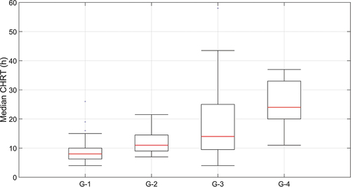
Figure 4. Box plots of estimated time to peak at watersheds within each group (see Section 4.4 for details) ranked in increasing values of median CHRT (black bars). Boxes correspond to the first (Q25) and third (Q75) interquartile ranges, and whiskers to 1.5 times the interquartile ranges [1.5 (Q75-Q25)]. Outliers (values larger or smaller than 1.5 (Q75-Q25)) are not shown. Median CHRT values in each group are represented by the vertical red dashed lines. The numbers next correspond to the watersheds discussed in Section 5.

4.2 Correlation with physiographic characteristics and comparison to empirical equations

Figure 5 shows the correlation based on linear regressions between CHRT and physiographic characteristics listed in Table 2. The highest coefficient of determination is associated with LW (R² = 0.28) followed by ${\text{L}}_{\text{C}}/\sqrt{{\text{S}}_{\text{C}}}$ (R² = 0.13). The possible influence of LW on CHRT is well documented (for lake: Hudson et al., 2021; for wetland: Kadykalo and Findlay, 2016). Still, very few empirical equations integrating LW as an explanatory variable have been proposed. In fact, of the 39 empirical equations listed in Gericke and Smithers (2014), only two used information related to LW. Kennedy and Watt (1967) considered the area of waterbodies in the upper two-third of the watershed, while Thomas et al. (2000) considered the lake and pond fraction. Also, Bell and Kar (1969) integrated a catchment storage coefficient, representing the retention and storage of the watershed without referring explicitly to LW.

Figure 5. Coefficient of determination (R²) of the linear regression between estimated CHRT and each physiographic characteristic (see Table 2). Only physiographic characteristics with R² > 0.005 are presented.

All other physiographic characteristics, except the connectivity between LW and the hydrographic network, have R² value lower than 0.05 and that include the main watercourse slope (S_C), the main watercourse length (L_C) and the watershed area (A) which often appears in documented empirical equations.

Figure 5 also shows that there is no significant correlation between the time to peak and the watershed area (R² < 0.005). This result may seem counterintuitive considering that area is a variable often included in many empirical equations (Mimikou, 1984; Williams, 1922; Wu, 1963; Gericke and Smithers, 2016b). However, it should be noted that areas of the watersheds in these studies varies over many orders of magnitude, for instance 202 to 5 005 km² for Mimikou, (1984), and 22 to 33 278 km² for Gericke and Smithers (2016b). This explains why watershed area comes out as an explanatory factor of CHRT. Limiting the analysis to watersheds less than 100 km² implies that other factors may be more influential than area on conditioning CHRT.

Observed CHRT were also compared to the estimated CHRT values estimated from empirical equations often mentioned in the literature (Espey et al. 1966; Kirpich, 1940; Williams, 1922; Wu 1963; FAA, 1970; Folmar and Miller, 2008; Haktanir and Sezen, 1990; Michaud et al. 2014; Mimikou, 1984; Sheridan, 1994). It shows that none of these formulations adequately reproduced the estimated CHRT values. Since most equations consider the same sets of physiographic characteristics as predictors, it is consistent with the previous result showing that CHRT is weakly correlated to the physiographic characteristics commonly considered in these equations (Figure 5).

4.3 Proposed regression tree to estimate the CHRT

Figure 6 presents the resulting regression tree, after imposing that all lower-level groups include at least 10 watersheds. The 21 physiographic characteristics listed in Table 2 were considered. The selected regression tree contains two hydrographic indicators and subdivide the initial set of watersheds into four groups with different CHRT. Accordingly, LW is the predominant physiographical characteristic explaining the hydrological response for the 93 watersheds. As expected, CHRT tends to increase as the fraction of LW increases. Comparing the estimated CHRT and observed median CHRT based solely on this first level division, a coefficient of determination of R² = 0.28 is obtained, a value similar to the one obtained using linear regression (Figure 5).

Figure 6. Regression tree to estimate CHRT for watersheds under study. Classification criteria appears on the first line in each box. First level of the regression tree considers the LW (lakes and wetlands) variable while the second level consider ${\text{L}}_{\text{C}}/\sqrt{{\text{S}}_{\text{C}}}$ (L_C: main watercourse length; S_C: main watercourse slope). Estimated watershed CHRT are indicated at the bottom-left of each box (median CHRT of watersheds of each group). The number of watersheds within each group is indicated in parenthesis.

Two elements may explain these results. First, LW cover large fractions of Quebec, Ontario and Canada watersheds (Kennedy and Meyer, 2002), as well as northeast United States watersheds (Tiner, 2010). Thirty-five out of the 93 watersheds (37.6%) under study have 10% or more of their surface covered by LW (Figure 2). Second, the LW plays a major role in watershed hydrological response as they can stock water and reduce peak flow and flood (Kadykalo and Findlay 2016). As a matter of fact, watershed response to specific events depends on antecedent moisture conditions (Branfireun and Roulet 1998), seasons (Quinton and Roulet, 1998) and localisation of the LW within the watershed (Hudson et al., 2021).

The next level of the regression tree involves the variable ${\text{L}}_{\text{C}}/\sqrt{{\text{S}}_{\text{C}}}$, which often appears in empirical equations. This variable is a proxy of the time taken by water to flow across the watershed. Inclusion of this variable in the regression tree improve the R² to 0.46. As can be seen lower ${\text{L}}_{\text{C}}/\sqrt{{\text{S}}_{\text{C}}}$ are associated to faster response and therefore shorter CHRT.

The third level of the regression tree identifies agricultural land use as a factor conditioning CHRT. The resulting tree encompasses five groups after group G-3 has been split into two groups according to agricultural land use (not shown on Figure 6). This level was not kept in the final regression tree as it leads to very little improvement of the R² (0.47 instead of 0.46 for the two-level regression tree). Further subdivisions result in a regression tree with less than 10 watersheds in some groups.

Figure 7 presents the resulting boxplots of the CHRT for the four groups (see also Figure 4). Dispersion of CHRT values is more pronounced for the G-3 group. Overlaps between the estimated values from different groups can be seen with an overall trend to larger CHRT from group 1 to 4.

Figure 7. Boxplots of the watershed median CHRT as classified by the regression tree (Figure 6). Horizontal red lines correspond to the estimated CHRT of each group.

Results indicate that, as for the CHRT, the fraction of LW is the leading factor explaining the interquartile ranges (R² = 0.24), watersheds with larger LW fraction having larger interquartile ranges (Figure 8). Thus, a large variability in initial storage conditions of lakes and wetlands will trigger very different responses and therefore a large variability in event based CHRT values (Bay,1969; Taylor and Pierson 1984; Roulet and Woo 1988).

Figure 8. Regression tree relating CHRT interquartile ranges to physiographic characteristics. Classification criteria appears on the first line in each box. First level of the regression tree considers the lakes and wetlands (LW) fraction, while the second level consider Agricultural (Agri) and Urban (U) fractions. Estimated interquartile ranges are indicated at the bottom-left of each box (median interquartile of each group). The number of watersheds within each group appears in parenthesis.

The next level involved agricultural and urban fractions, two land uses associated with quick hydrological response (Figure 8). The increases in performance remain small compared to the first level (R² = 0.33) but results are consistent with hydrological intuition. Thus, watersheds with small LW coverage (< 10%) are subdivided according to the fraction of agricultural land while those with larger LW coverage (≥ 10%) are subdivided according to their urban fraction. In both case, fast responses, and less event dependent CHRT, are associated to watersheds with larger agricultural or urban covers.

4.4 Uncertainties on estimated CHRT

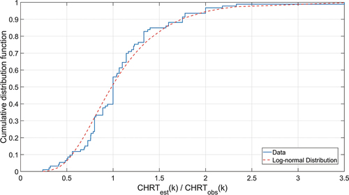
Figure 9 presents the cumulative distribution function (CDF) of the ratios between estimated CHRT and observed CHRT (equation 1(1) ${\text{R}}_{\text{k}}=\frac{{\text{CHRT}}_{\text{est}}\left(\text{k}\right)}{{\text{CHRT}}_{\text{obs}}\left(\text{k}\right)}$(1) ) for all 93 watersheds. A log-normal distribution (mean = 1.08; standard deviation = 0.72) has been adjusted to this sample. Median value of the distribution is at ${\text{R}}_{\text{k}}=1$ meaning that there is an equal probability that the estimated value be higher or lower than the observed one. It also shows that the estimated values can be quite uncertain. Despite these large uncertainties, this distribution is however useful as it provides guidelines on safety margins that could be applied by practitioners in situation where underestimated or overestimated CHRT may result in unacceptable risks.

Figure 9. Cumulative distribution function of the ratios between the estimated and observed CHRT, CHRT_est(k)/ CHRT_obs(k), for 93 watersheds under study. Dashed line corresponds to a log-normal distribution fitted to the data ($\mathit{\mu }=-0.02;\mathit{\sigma }=0.44)$.

4.5. Further investigation of specific watersheds

Observed CHRT at some watersheds are significantly different from estimated CHRT. These differences may be explained by some peculiar physiographic characteristics having a major impact on the watershed hydrological response, which is not accounted for, or uniquely present in a few watersheds, and therefore doesn’t come out from the previous analysis. Six watersheds, identified on Figure 4, are therefore further discussed to better understand, and explained these differences.

The largest CHRT overestimation among the 93 watersheds is for the watershed upstream of station 02DB007 in Ontario classified in group 4 (Figure 4). The area of this watershed is 69.4 km² and it is mainly covered by forest (81.6%). The observed CHRT is 11 hours, while the estimated CHRT is 28 hours, an underestimation of 17 hours. A close look at this watershed shows that many rock outcrops, mostly granite and gneiss, are exposed over large area of the watershed, resulting in large runoff volume and fast hydrological response (Onda et al., 2001). This feature is accounted for by the hydrological soil categories (Table 2). This watershed is mainly associated to category CD, a unique feature among the watersheds. Therefore, despite a LW coverage larger than 10% (11.4%) and a large ${\text{L}}_{\text{C}}/\sqrt{{\text{S}}_{\text{C}}}$ value (36.2 km), the presence of large rocky outcrops may explain the large CHRT overestimation in that case.

The presence and location of urban area in some watershed may also explain why CHRT differ significantly from the estimated value, since urban fraction was not globally identified as a predictive factor. As a reminder, urban fractions are small for a vast majority of watersheds (less than 2.5% for half of the basins; see Figure 2). However, urban areas cover 14.4% of the watershed upstream of station 02HB012 in Ontario, the third largest urban fraction among the 93 watersheds. This watershed is the one with the smallest observed CHRT of group 3 with an observed CHRT of 6 hours. CHRT value is therefore overestimated by 11 hours (Figure 4). In addition, urban areas are in the downstream portion of the watershed, while the LW (15.7%) are in the upper part of the basin. Such configuration likely favors a quick hydrological response, despite a larger LW fraction (15.7%). Therefore, the presence and relative location of urban area in the watershed counterbalance the ‘LW effect’ and results in a much shorter response than estimated. Complex hydrographs characterized by a first quick and high peak flow followed by a smaller were also observed for this watershed (Yang et al., 2015).

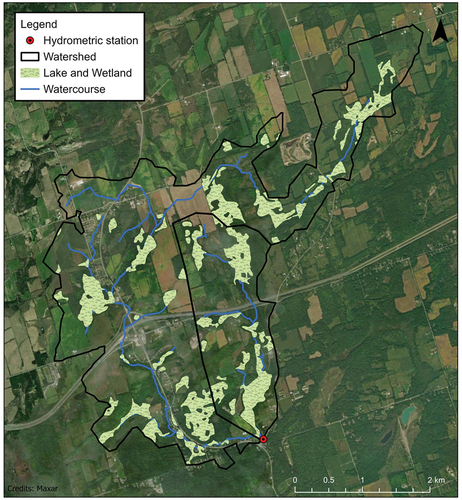
Another peculiar feature seen in some watersheds which has a major impact on response time and on the structure of the hydrographs, is the division of the hydrographic network in distinct sub-networks close to the outlet. Such feature is observed for the watershed upstream of station 02HD018 in Ontario (15 km²; Figure 10). In that case the estimated CHRT is 17 hours, while the observed value is 6 hours, the second smallest observed CHRT of group G-3 (Figure 4). As seen on Figure 10, the watershed is subdivided into two sub-watersheds with significantly different land uses just upstream the station. Such configuration may therefore explain the quicker than anticipated response time of this watershed especially from the left-hand side sub-watershed dominated by agricultural lands.

Figure 10. Watershed and sub-watersheds upstream of station 02HD018 in Ontario.

Six sub-watersheds from the lake-stream network at the Turkey lakes watershed in central Ontario (Canada) were considered in this study. The hydrological response of these watersheds was analyzed by Hudson et al. (2021). A very complex interaction between hydrological response and precipitation was revealed by this study, which also provided evidence that stations closer to lake outlet have smoother peak flow response (see also Leach and Laudon, 2019). In fact, the biggest underestimation comes from one of these watersheds, the one upstream of station 02BF007 (5.1 km²) identified as 07 on Figure 1 of Hudson et al. (2021) for which the median observed CHRT is 58 hours and the estimated one is 14 hours (Group G-3; Figure 6). This difference is likely due to the proximity of the station from the lake outlet. Observed CHRT are also underestimated, although to a lesser extent, for sub-watersheds upstream of stations 02BF008 (3.5 km²; group G-3), and 02BF009 (2.1 km²; group G-1), presumably for the same reasons. These results show that the location of the lakes relative to the station may have a significant impact on the hydrological response as pointed out by Hudson et al. (2021). A larger sample of watersheds with more diverse watershed LW distribution would be necessary to globally capture and quantify this influence.

The storage capacity of LW can also play a crucial role in the watershed response (Quin and Destouni, 2018). The watershed with the highest LW occupation (18%) upstream of station 050813 (Québec; 2 km²) has an observed median CHRT of 17 hours, a value like many other watersheds without LW. This very small watershed is characterized by the presence of a single lake with very steep banks located in the central part of the watershed. The storage capacity of the lake is therefore small (no flood plain around the lake) and this may explain the relatively quick hydrological response of the watershed compared to other watersheds with similar LW percentage. In contrast, the 6.5 % of LW for the watershed upstream of station 040212 (Québec, 40 km²) are in the central and upstream parts of the watershed. The observed CHRT of this watershed is 26 hours, a much larger value than the estimated value of 8 hours, the largest overestimation for group G-1 (Figure 6). In that case, even if the LW aren’t located near the station, 66% of the watershed area is drained by these lakes. In addition, the LW are in a very flat zone with a large floodplain and likely a large land surface storage capacity. It is important to mention that even if these considerations relate to lakes, similar conclusions can be reached for wetlands (Acreman and Holden, 2013; Ahlén et al., 2022).

5. Summary and conclusion

Time of concentration is a useful concept in applied hydrology. It is often used by practitioners having to design various hydraulic infrastructures, for instance when applying the rational method. Many empirical equations, still widely used, have been proposed to estimate the time of concentration from the physiographic characteristics of a watershed. The time of concentration may therefore be interpreted as a characteristic hydrological response time (CHRT) averaged over a large sample of hydro-meteorological conditions. In absence of any local information, practitioners sometimes apply these equations, usually developed for watersheds with specific characteristics and exposed to peculiar climate conditions, to watersheds with very different attributes and climatic conditions. This practice is obviously questionable as it remains preferable, even if it may be challenging, to develop empirical equations based on local dataset. This is the object of this study.

A total of 93 small watersheds, ranging from 0.6 to 100 km² with 15-min time step recorded flow series from June 1^st to October 31^st (period without snowmelt and ice cover) in Canada (Ontario and Quebec) and the northeastern USA (Maine Vermont, New York, and Massachusetts) was considered. Annual maxima flow over the June to October period were extracted at each station. These watersheds are mainly covered with forest, while lakes and wetlands (LW) are present in almost all catchments (89 out of 93). Urban areas are marginal (median of 6%) with no watershed having more than 17% of urban areas.

The Smoothed Minima Baseflow Separation (SMBS) method, adapted to sub-hourly flow records, was used to extract the hydrographs from the flow records. An average of 2.5 single and two-peak hydrographs associated to the largest annual recorded flows were extracted at each watershed (38 hydrographs/watershed on average).

Times to peak of each selected hydrograph were estimated. Median values of hydrograph times to peak distribution at each watershed were used as estimates of the watershed CHRT, hereafter called observed CHRT. Dispersion of hydrograph times to peak values at each watershed can be larger than the variability of observed CHRT between watersheds, showing that CHRT are highly uncertain and strongly hydrograph-dependant.

Observed CHRT were then related to physiographic characteristics. Comparison to available empirical equations proposed in the literature shows that none of the equations adequately reproduced the observed CHRT. Regression trees were then used to identify the main factors conditioning CHRT of each watershed. The developed regression tree encompasses four groups with CHRT values of 8 hours (group G-1), 11 h (group G-2), 14 h. (group G-3), and 24 hours (group G-4). CHRT is a function of two physiographic characteristics: 1) the fraction of LW at the first level of the regression tree; 2) the ratio between the main watercourse length and the square root of the main watercourse slope (${\text{L}}_{\text{C}}/\sqrt{{\text{S}}_{\text{C}}}$) at the second level. This last expression appears in many empirical equations relating CHRT to physiographic characteristics.

Uncertainties on estimated CHRT were then assessed. The ratio of estimated (CHRT_est) and observed (CHRT_obs) CHRT, CHRT_est/CHRT_obs, were computed and adjusted to a log-normal distribution. As expected, uncertainties on estimated CHRT are significant. For instance, there is a 5% probability that observed CHRT be larger than twice the estimated CHRT. Providing guidelines on uncertainties on estimated CHRT is therefore even more important and could be used by practitioners to define security factors in situation where underestimated or overestimated CHRT, and corresponding designed hydraulic capacities, may have major consequences and lead to unacceptable risks.

A more comprehensive investigation of watersheds where estimated CHRT largely overestimated or underestimated observed CHRT was carried out. In all cases, differences may be attributed to peculiar characteristics that have a major impact on the hydrological response. These features may be related to land use (e.g., large scale exposed rock outcrops), the presence and location of urban area within the watershed, the subdivision of the watershed in sub-watersheds with different land uses close to the outlet, or the location and storage capacities of LW. Some of these features were not, or inadequately, accounted for by selected physiographic characteristics, while some were unique or present in a few watersheds, and therefore not identified as predictors of CHRT. These few examples show that multiple and opposing factors may have an impact on the hydrological response of specific watersheds and that caution and professional judgement are recommended when estimating CHRT.

Finally, it is crucial to remind that the developed regression tree is based on a specific set of small watersheds located in Northeastern North America. Transposability of the approach to watersheds located elsewhere is possible, but an application per se of the estimated CHRT is not suggested.

Future research should investigate how to increase the number of watersheds under study and possibly includes watersheds located in other climatic zones. New physiographic characteristics could also be integrated into the analysis. Finally, the possibility to use gridded datasets (Gasset et al., 2021) to further investigate the meteorological conditions associated to peak flows could help improve our understanding of the watershed hydrological response and identify key factors conditioning the CHRT.

Acknowledgements

The authors would like to thank the organizations and persons who provided the dataset used in this study: Louis Duchesne and Jean-Pierre Saucier from Direction de la recherche forestière du Ministère des Forêts, de la Faune et des Parcs (MFFP) as well as Alton Stead and Melanie Taylor from Environment and Climate Change Canada (ECCC). The authors also thank the Ministère des Transport du Québec who funded this project. Finally, Alain Mailhot thanks the Discovery Grants Program from the Natural Science and Engineering Research Council of Canada (NSERC) for partly providing financial support for this project.

Supplementary material

Supplemental data for this article can be accessed online at https://doi.org/10.1080/02626667.2024.2387155.

References

- Acreman, M. and Holden, J. 2013. How wetlands affect floods. Wetlands, 33 (5), 773-786. doi: 10.1007/s13157-013-0473-2
- Ahlén, I. et al. 2022. Wetland position in the landscape: Impact on water storage and flood buffering. Ecohydrology, 15 (7), e2458. doi: 10.1002/eco.2458
- Bay, R.G. 1969. Runoff from small peatland watersheds. Journal of Hydrology, 9 (1), 90-102. doi: 10.1016/0022-1694(69)90016-X
- Bell, F.C. and Karr, S.O. 1969. Characteristic response times in design flood estimation. Journal of Hydrology, 8 (2), 173–196. doi:10.1016/0022-1694(69)90120-6
- Beven, K.J. 2020. A history of the concept of time of concentration. Hydrology and Earth System Sciences, 24 (5), 2655–2670. doi: 10.5194/hess-24-2655-2020
- Branfireun, B.A. and Roulet, N.T. 1998. The baseflow and storm flow hydrology of a precambrian shield headwater peatland. Hydrological Processes, 12 (1), 57-72. doi: 10.1002/(SICI)1099-1085(199801)12:13.0.CO;2-U
- Breiman, L. et al. 1984. Classification and Regression Trees. Chapman & Hall, Boca Raton, FL, 368 p.
- Dhakal, N. et al. 2013. Rate-based estimation of the runoff coefficients for selected watersheds in Texas. Journal of Hydrologic Engineering, 18 (12), 1571-1580. doi: 10.1061/(ASCE)HE.1943-5584.0000753
- Dibike, Y.B. et al. 2021. Assessing climatic drivers of spring mean and annual maximum flows in western Canadian river basins. Water, 13 (12), 1617. DOI: 10.3390/w13121617
- Espey, Jr. W.H. Morgan, C.W. and Masch, F.D. 1966. A study of some effects of urbanization on storm runoff from a small watershed. Texas water development board, Report 23, Texas University, 110 p.
- FAA, 1970. Airport drainage. AC 150/5320-5B. Department of transportation. United-States federal aviation administration. Washington. D.C. 80 p.
- Folmar N.D. and Miller A.C. 2008. Development of an empirical lag time equation. Journal of Irrigation and Drainage Engineering, 134 (4), 501-506. doi: 10.1061/(ASCE)0733-9437(2008)134:4(501)
- Gagné G. et al. 2013. Classement des séries de sols minéraux du Québec selon les groupes hydrologiques. Rapport final, IRDA, Québec, Canada, 81 p.
- Gasset N. et al. 2021. A 10 km North American Precipitation and Land Surface Reanalysis Based on the GEM Atmospheric Model. Hydrology and Earth System Sciences, 25 (9), 4917-4945. doi: 10.5194/hess-2021-41
- Gericke O.J. and Smithers J.C. 2016a. Are estimates of watershed response time inconsistent as used in current flood hydrology practice in South Africa. Journal of the South African Institution of Civil Engineering, 58 (1), 2-15. doi: 10.17159/2309-8775/2016/v58n1a1
- Gericke O.J. and Smithers J.C. 2016b. Derivation and verification of empirical watershed response time equations for medium to large catchments in South Africa. Hydrological Processes, 30 (23), 4384-4404, doi: 10.1002/hyp.10922
- Gericke O.J. and Smithers J.C. 2014. Review of methods used to estimate watershed response time for the purpose of peak discharge estimation. Hydrological Sciences Journal, 59 (11), 1935-1971. doi: 10.1080/02626667.2013.866712
- Grimaldi, S. and Petroselli, A. 2015. Do we still need the Rational Formula? An alternative empirical procedure for peak discharge estimation in small and ungauged basins. Hydrological Sciences Journal, 60 (1), 67-77. doi: 10.1080/02626667.2014.880546
- Grimaldi S. et al. 2012. Time of concentration: a paradox in modern hydrology. Hydrological Sciences Journal, 57 (2), 217-228. doi: 10.1080/02626667.2011.644244
- Hatkanir, T. and Sezen, N. 1990. Suitability of two-parameter gamma and three parameter beta distributions as synthetic unit hydrographs in Anatolia. Hydrological Sciences Journal, 35 (2), 167-184. doi: 10.1080/02626669009492416
- Hotchkiss, R.H. and Mc Callum, B.E. 1995. Peak Discharge for small agricultural watersheds. Journal of Hydraulic Engineering, 121 (1), 36-48. doi: 10.1061/(ASCE)0733-9429(1995)121:1(36)
- Hudson, D.T. et al. 2021. Streamflow regime of a lake-stream system based on long-term data from a high-density hydrometric network. Hydrological Processes, 35 (10), e14396. doi: 10.1002/hyp.14396
- Institute of hydrology (1980). Low flow studies, Report No 1. Research report, Crowmarsh Gifford, Wallingford, Oxon, 42 p.
- Jena, M. and Dehuri, S. 2020. Decision tree for classification and regression: A state-of-the Art review. Informatica, 44, 405-420. doi: 10.31449/inf.v44i4.3023
- Kadykalo, A.N. and Findlay, C.S. 2016. The flow regulation services of wetlands. Ecosystem Services, 20, 91-103. doi: 10.1016/j.ecoser.2016.06.005
- Kennedy, G. and Mayer, T. 2002. Natural and constructed wetlands in Canada: An overview. Water Quality Research Journal of Canada, 37 (2), 295-325. doi: 10.2166/wqrj.2002.020
- Kennedy, R.J. and Watt, W.E. 1967. The relationship between lag time and the physical characteristics of drainage basins in Southern Ontario. International Association of Scientific Hydrology, Symposium on Flood and their computation, 85, 866-874.
- Kerby, W.S. 1959. Time of concentration for overland flow. Civil Engineering, 26 (3), 59-60.
- Kirpich Z.P. 1940. Time of concentration of small agricultural watersheds. Civil Engineering, 10 (6), 362.
- Leach, J.A. and Laudon, H. 2019. Headwater lakes and their influence on downstream discharge. Limnology and Oceanography Letters, 4 (4), 105-112. doi: 10.1002/lol2.10110
- Loh, W.Y. 2011. Classification and regression trees. WIREs Data Mining and Knowledge Discovery, 1 (1), 14-23. doi: 10.1002/widm.8
- Mailhot, A. et al. 2021. Révision des critères de conception des ponceaux pour des bassins de drainage de 25 km2 et moins dans un contexte de changements climatiques (CC06.2). Rapport Final, Institut National de la Recherche Scientifique INRS-Eau, Terre et Environnement, Québec, mars 2021, 291 p. (in French).
- Mailhot, A. Bolduc, S. and Talbot, G. 2018. Révision des critères de conception des ponceaux pour des bassins de drainage de 25 km2 et moins dans un contexte de changements climatiques (CC06.1). Rapport Final, Institut National de la Recherche Scientifique INRS-Eau, Terre et Environnement, Québec, mars 2018 (In French).
- McCuen, R.H. 2009. Uncertainty analyses of watershed time parameters. Journal of Hydrologic Engineering, 14 (5), 490-498. doi: 10.1061/(ASCE)HE.1943-5584.0000011
- McCuen R.H. Wong S.L. and Rawls W.J. 1984. Estimating urban time of concentration. Journal of Hydraulic Engineering, 110 (7), 887-904.
- Michailidi, E.M. et al. 2018. Timing the time of concentration: shedding light on a paradox. Hydrological Sciences Journal, 63 (5), 721-740, doi: 10.1080/02626667.2018.1450985
- Michaud, A.R. et al. 2014. Développement et validation de méthodes de prédiction du ruissellement et des débits de pointe en support à l’aménagement hydro-agricole. Rapport final, Institut de recherche et de développement en agroenvironnement inc. (IRDA), Québec, Canada, 142 pp (in French).
- Michelon, A. et al. 2021. Benefits from high-density rain gauge observations for hydrological response analysis in a small alpine catchment. Hydrology and Earth System Sciences, 25 (4), 2301-2325. doi: 10.5194/hess-25-2301-2021
- Mimikou, M. 1984. Regional relationships between basin size and runoff characteristics. Hydrological Sciences Journal, 29 (1), 63-73. doi: 10.1080/02626668409490922
- MTO (1997). Drainage management manual. Part 3, Chapter 8, Drainage and hydrology section, Transportation engineering branch, Quality and standards division, Ministry of Transportation Ontario. 184 p.
- Mulvany, T. J. 1851. On the use of self-registering rain and flood gauges in making observations of the relations of rainfall and flood discharges in a given catchment. Proceeding Institution of Civil Engineers of Ireland, 4 (2), 18–33.
- Nathan, R.J. and McMahon, T.A. 1990. Evaluation of automated techniques for base flow and recession analyses. Water Resources Research, 26 (7), 1465-1473, doi: 10.1029/WR026i007p01465
- Newman, A.J. 2019. Methodological intercomparisons of station-based gridded meteorological products: Utility, limitations, and paths forward. Journal of Hydrometeorology, 20 (3), 531-547. doi: 10.1175/JHM-D-18-0114.1
- Onda, Y. et al. 2001. The role of subsurface runoff through bedrock on storm flow generation. Hydrological Processes, 15 (10), 1693-1706. doi: 10.1002/hyp.234
- Paschalis, A. et al. 2014. On the effects of small scale space-time variability of rainfall on basin flood response. Journal of Hydrology, 514, 33-327. doi: 10.1016/j.jhydrol.2014.04.014
- Pilgrim. D.H. and Cordery, I. 1993. Chapter 9: Flood runoff. In Maidment, D.T. Handbook of hydrology. McGraw-Hill, New-York, USA.
- Quin, A. and Destouni, G. 2018. Large-scale comparison of flow-variability dampening by lakes and wetlands in the landscape. Land Degradation & Development, 29, 3617-3627. doi: 10.1002/ldr.3101
- Quiton, W.L. and Roulet, N.T. 1998. Spring and summer runoff hydrology of a subarctic patterned wetland. Arctic and Alpine Research, 30 (3), 285-294. doi: 10.2307/1551976
- Ramser, C.E. 1927. Run-off from small agricultural areas. Journal of Agricultural Research, 34 (9), 797-823.
- Ravazzani, G. et al. 2019. Review of Time-of-Concentration Equations and a New Proposal in Italy. Journal of Hydrologic Engineering, 24 (10), 04019039. doi: 10.1061/(asce)he.1943-5584.0001818
- Rossmiller R. 1980. The rational formula revisited. International symposium on urban storm runoff, University of Kentucky, Lexington, Kentucky, July 28-31, 1980, p. 1-12.
- Roulet, N.T. and Woo, M.K. 1988. Runoff generation in low arctic drainage basin. Journal of Hydrology, 101 (1-4), 213-226. doi: 10.1016/0022-1694(88)90036-4
- Sheridan J.M. 1994. Hydrograph time parameters for flatland watershed. Transactions of the ASCE, 37 (1), 103-113.
- Singh V.P. 1997. Effect of spatial and temporal variability in rainfall and watershed characteristics on stream flow hydrograph. Hydrological Processes, 11 (12), 1649-1669. doi: 10.1002/(SICI)1099-1085(19971015)11:12<1649::AID-HYP495>3.0.CO;2-1
- Singh, V.P. 1988. Hydrologic systems: Volume 1, Rainfall-runoff modeling. Prentice Hall, Englewood Cliffs, New Jersey, 480 p.
- Tarasova, L. et al. 2018. Exploring controls on rainfall-runoff events: 1. Time series-based event separation and temporal dynamics of event runoff response in Germany. Water Resources Research, 54 (10), 7711–7732, doi: 10.1029/2018WR022587
- Taylor, C.H. and Pierson, D.C. 1984. The effect of a small wetland on runoff response during spring snowmelt. Atmosphere-Ocean, 23 (2), 137-154.
- Thomas, Jr. W.O. Monde, M.C. and Davis, S.R. 2000. Estimation of time of concentration for Maryland streams. Transportation Research Record, 1720 (1), 95-99. doi: 10.3141/1720-11
- Tiner, R. 2010. Wetlands of the Northeast: Results of the National Wetlands Inventory. U.S. Fish and Wildlife Service, Northeast Region, Hadley, MA. 71 p.
- Transports Québec, 2017. Manuel de conception des ponceaux. Ministère des transports du Québec, Division des structures, 541 p.
- USBR, 1973. Design of small dams. 2nd ed. Washington, DC: Water Resources Technical Publications, United States Bureau of Reclamation.
- Williams G.B. 1922. Flood discharge and the dimensions of spillways in India. The Engineer, Sept. 29, 321-322.
- Wu, I.P. 1963. Design hydrographs for small watershed in Indiana. Journal of Hydraulic Engineering, 89 (6), 35-66.
- Xie, J. et al. 2020. Evaluation of typical methods for baseflow separation in the contiguous United States. Journal of Hydrology, 583, 124628. doi: 10.1016/j.jhydrol.2020.124628
- Yang, Y. Endreny, T.A. and Nowak, D.J. 2015. Simulating double-peak hydrographs from single storms over mixed-used watersheds. Journal of Hydrologic Engineering, 20 (11), Technical note. doi: 10.1061/(ASCE)HE.1943-5584.0001225
- Young, C.B. and McEnroe, B.M. 2014. Evaluating the form of the rational equation. Journal of Hydrologic Engineering, 19 (1), 265-269. doi: 10.1061/(ASCE)HE.1943-5584.0000769
- Young, C.B. McEnroe, B.M. and Rome, A.C. 2009. Empirical determination of rational method runoff coefficient. Journal of Hydrologic Engineering, 14 (12), 1283-1289. doi: 10.1061/(ASCE)HE.1943-5584.0000114