Criterion validity of neural networks to assess lower limb motion during cycling

ABSTRACT

The use of marker-less methods to automatically obtain kinematics of movement is expanding but validity to high-velocity tasks such as cycling with the presence of the bicycle on the field of view is needed when standard video footage is obtained. The purpose of this study was to assess if pre-trained neural networks are valid for calculations of lower limb joint kinematics during cycling. Motion of twenty-six cyclists pedalling on a cycle trainer was captured by a video camera capturing frames from the sagittal plane whilst reflective markers were attached to their lower limb. The marker-tracking method was compared to two established deep learning-based approaches (Microsoft Research Asia-MSRA and OpenPose) to estimate hip, knee and ankle joint angles. Poor to moderate agreement was found for both methods, with OpenPose differing from the criterion by 4–8° for the hip and knee joints. Larger errors were observed for the ankle joint (15–22°) but no significant differences between methods throughout the crank cycle when assessed using Statistical Parametric Mapping were observed for any of the joints. OpenPose presented stronger agreement with marker-tracking (criterion) than the MSRA for the hip and knee joints but resulted in poor agreement for the ankle joint.

KEYWORDS:

• Movement analysis
• bicycle
• machine learning
• joint kinematics

Introduction

The assessment of posture on the bicycle has been used extensively with the purpose of reducing injuries and improving performance (Holliday & Swart, 2021; R. R. Bini et al., 2011). This assessment involves measuring joint angles and mapping them against recommended ranges of motion proposed in the literature (R. Bini & Priego-Quesada, in press; Swart & Holliday, 2019). Obtaining joint kinematics data involves using video analysis to identify bony landmarks. This process is time consuming because it requires accurate palpation of skin landmarks to ensure that marker position reflects skeletal tracking during motion (Szczerbik & Kalinowska, 2011). Therefore, minimizing the time required and errors from marker placement could improve the accuracy of measurements.

Marker-less methods have been explored to obtain joint kinematics in prior studies (D’antonio et al., 2021; Needham et al., 2021; Ong et al., 2017; Pagnon et al., 2022; Serrancolí et al., 2020). However, only Serrancolí et al. (2020) and R. R. Bini et al. (2022) utilized pre-trained convolution neural networks (CNN) based approaches to identify segmental movement and joint centres during cycling with the purpose of tracking movement. This is beneficial because, compared to other methods such as optoelectronic systems and inertial measurement units (IMU), marker-less methods obtained from standard video camera footage could reduce time required in preparing the cyclist for the assessment, which facilitates clinical use. As an example, changes in body posture on the bicycle (bike fitting) could be streamlined using valid mark-less methods. Differently, optoelectronic systems and IMUs require specific sensors for data collection whilst CNN can be employed more flexibly in standard video footage taken from smartphones (e.g., OpenCap – Musculoskeletal forces from smartphone videos.). More importantly, using pre-trained CNN from open-source software could enable customisation of outputs tailored to specific needs of cyclists. This approach could involve determining key outcomes from movement (e.g., minimum and maximum flexions and extensions) provided to the practitioner for easier use. However, comparison with criterion methods (i.e., marker-based) is missing for cycling given neural networks use different assumptions in determining joint centres. Even though prior studies demonstrated strong agreement between marker-less methods and movements like running (Johnson et al., 2022; Ota et al., 2021), squatting (Ota et al., 2020) and jumping (Drazan et al., 2021) in relation to sagittal plane marker tracking, these studies utilized high frame rate (i.e., 60–125 fps) obtained with relatively high image resolution (e.g., 800 × 600). In addition, only Drazan et al. (2021) analysed the agreement of waveforms with no data on higher velocity tasks such as cycling. Finally, the presence of the bicycle in the field of view could be an element affecting the accuracy of the CNNs to properly identify cyclists’ body segments.

In cycling, performance of two pre-trained CNN methods (i.e., Microsoft Research Asia – MSRA and OpenPose) has been shown to be promising in determining joint angles at two points of the crank cycle (i.e., 3’clock and 6 o’clock; R. R. Bini et al., 2022). However, this study was limited to only two time points (i.e., no temporal comparison with the marker data) and used 120 fps, which limits the application of data to video obtained from lower-cost smartphone cameras and webcams (i.e., 30 fps and standard video resolution − 640 × 480 pixels). Therefore, employing a statistical parametric mapping method (i.e., SPM; Pataky et al., 2013) could provide a temporal comparison between methods to fully determine sections of the crank cycle where a given method is less accurate. This is important to analyse movement patterns, which are sensitive to exercise intensity (Holliday et al., 2019; R. R. Bini & Diefenthaeler, 2010), cadence (R. R. Bini, Rossato, et al., 2010), fatigue (R. R. Bini, Diefenthaeler, et al., 2010; Sayers & Tweddle, 2012), and body position on the bicycle (Ferrer-Roca et al., 2014; R. R. Bini et al., 2014) and can contribute to better inform technique training strategies.

Thus, this study was conducted to determine the criterion validity of two open-source convolutional neural networks (MSRA and OpenPose) in determining joint angles during stationary cycling. Even though both neural networks have not been potentially pre-trained using images of people cycling, our hypothesis was that both methods would produce good to excellent agreement with the criterion in determining joint angles during cycling. In order to compare implications for traditional zero-dimensional measures (R. R. Bini et al., 2012, 2016), we also assessed the agreement from these neural networks in terms of mean angles and ranges of motion.

Materials and methods

Twenty-six cyclists (22 males and four females, 37 ± 10 years of age, 178 ± 9 cm of stature and 80 ± 11 kg of body mass) ranging from recreational to competitive were assessed in a single session using their own bicycles. Cyclists should not be experiencing pain, injury or chronic conditions that would affect their exercise regime. Before data collection, all cyclists signed an informed consent to participate in the study, which was approved by the University Human Ethics Committee (AUTEC09/178). The sample size was calculated utilizing an ANOVA for repeated measurements (within factors) with an effect size of 0.735 (adapted from R. R. Bini et al., 2022) to compare three methods (criterion, MSRA and OpenPose) with a correlation for repeated measures of 0.30 (Burnie et al., 2020) and α < 0.05 and power of 0.80 using G*Power statistical package (Faul et al., 2007). Because the required sample would be only six participants, we expanded the sample to account for a larger sample size required to analyse waveforms (Robinson et al., 2021).

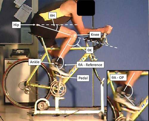
After measurements of stature and body mass, cyclists performed 2-min of cycling on their own bicycles attached to a cycle trainer (Kingcycle, Buckinghamshire, UK) at self-selected cadence. Participants were instructed to sustain an intensity equivalent to a long duration flat cycling. A digital camera (Samsung ES15, Seoul, South Corea) was positioned at the height of their saddle, 4-m away from the bicycles to record movement in the sagittal plane. Reflective markers were attached by a trained investigator to the greater trochanter, lateral femoral epicondyle, lateral malleolus and pedal spindle (Figure 1). Videos were recorded for 20-s at the end of the 2-min of exercise at 30 fps (640×480 of frame resolution) using automated quick shutter and anti-shake settings to minimize blur. The option for standard video rather than high-speed intended to simulate specifications of most lower-cost smartphone video cameras.

Figure 1. Illustration of the kinematic model used to calculate hip (θH), knee (θK) and ankle (θA) angles. Inset illustrates model used for measuring the ankle angle using OpenPose (OP).

The results obtained using OpenPose and the MSRA methods were compared, which are a bottom-up and top-down deep learning-based approach designed to estimate human pose. These include open-source code with a very large number of users currently exploring the utility of these CNNs and consolidated algorithm with adapted platforms for various users (e.g., Windows, Ubunty, Mac, etc.). In addition, the MSRA presents a very fast processing CNN with easy implementation using Matlab of deployable tools (Markless Motion Analyser – File Exchange – MATLAB Central (mathworks.com)).

The MSRA method first detects the location of multiple people in an image, and then the body parts for each detected person. Differently, OpenPose computes a confidence map that gives the location of the body parts and a set of vector fields. Video files were then imported to a customized program adapted from a shared code. This code implements the MSRA method (Xiao et al., 2018) in MATLAB (R2021a, MathWorks Inc, Natick, MA, USA). For OpenPose, video files were processed in Canonical Ubuntu 20.04 LTS (Kernel GNU/Linux 5.4) using a customized Docker image (exsidius/openpose) to provide a matrix with the image coordinates for each key-point detected over time. In this study, OpenPose and the MSRA methods used models pre-trained in the COCO Consortium (cocodataset.org) (Lin et al., 2014) a markerless-based keypoint dataset containing labelled human joints in an uncontrolled and challenging environment whose annotations were obtained using a crowd labelling strategy on Amazon Mechanical Turk. In our study, the predicted joint centres (i.e., keypoints) were obtained from both methods and utilized to calculate hip, knee and ankle angles, as shown in Figure 1. Ankle angles were not calculated for the MSRA because this method did not identify the foot. Keypoints were gap filled using a 1d-median filter and a 3-samples moving average was utilized to reduce noise from the automated digitization prior to angular calculations.

As a criterion measure, hip, knee and ankle angles were also calculated using reflective markers digitized from each frame. Semi-automatic digitization was performed using a motion analysis software (Skill Spector, Video4Coach, Denmark). The median filter and moving average were also applied to the digitised joint centres in order to reduce filtering effects to comparisons with the OpenPose and MRSA methods. An offset was applied to the OpenPose ankle angles because these angles were measured differently to the reference (criterion) method, where the ankle was determined using the pedal axle (see Figure 1). Data from the two methods and the criterion were sectioned into ten consecutive crank cycles (from top dead centre to the following top dead centre position), with the mean temporal series from each cyclist obtained for further analysis. All data was time normalised to 360 points, one sample for each degree of the crank angle. Mean angle and range of motion from each joint was extracted for statistical analysis.

Comparison of temporal patterns was performed between methods using statistical parametric analyses within spm1d statistical package (www.spm1d.org), in MATLAB. Repeated measures ANOVAs were employed to assess the differences between methods in joint angles followed by Post Hoc comparisons (with Bonferroni corrections), whenever main effects were significant (α<0.05), using paired samples t-tests. Intraclass correlation coefficients (ICC) were calculated for each crank angle for the “A-1” method (criterion-referenced) using an open-source code (https://www.mathworks.com/matlabcentral/fileexchange/22099-intraclass-correlation-coefficient-icc). ICC values less than 0.5 were indicative of poor reliability, values between 0.5 and 0.75 indicate moderate reliability, values between 0.75 and 0.9 indicate good reliability, and values greater than 0.90 indicate excellent reliability (Koo & Li, 2016). Minimum detectable changes (MDC) were calculated from the pooled standard error and ICCs, as described in (Suriyaamarit & Boonyong, 2018). Finally, Bland and Altman plots were produced to examine mean bias and limits of agreement between neural networks and the creation for mean angles and ranges of motion from each joint.

Results

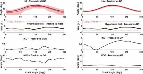
No significant differences were observed between the criterion and the MSRA method for the hip angle (Figure 2). Largest ICC was poor (0.27) and minimum detectable change ranged between 14–31°. Comparison between the criterion and OpenPose also have not produced significant differences. Largest ICC was moderate (0.77) and minimum detectable change ranged between 4–8°.

Figure 2. Left panel shows hip angle (HA) temporal comparison between criterion (Tracked – black) and MSRA (MSR – red) methods whilst right panel shows comparison between criterion (Tracked – black) and OpenPose (OP – red). SPM 1-d statistics is shown at the second level, with alpha (α) value from the Bonferroni correction indicated in dashed lines. Solid lines present the t statistic outputs from the post hoc analyses whilst the dashed red lines show the critical t value for significant differences. Intraclass correlation coefficients (ICC) across the crank cycle are shown in the third level and minimum detectable change is shown at the fourth level.

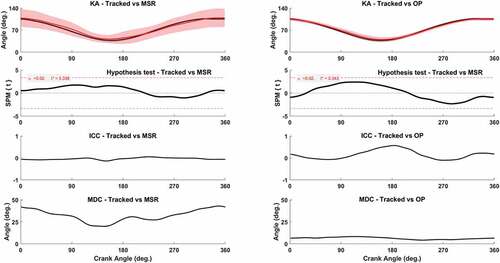
No significant differences were observed between the criterion and the MSRA method for the knee angle (Figure 3). Largest ICC was poor (0.05) and minimum detectable change ranged between 19–42°. Comparison between the criterion and OpenPose also have not produced significant differences. Largest ICC was moderate (0.57) and minimum detectable change ranged between 4–8°.

Figure 3. Left panel shows knee angle (KA) temporal comparison between criterion (Tracked – black) and MSRA (MSR – red) methods whilst right panel shows comparison between criterion (Tracked – black) and OpenPose (OP – red). SPM 1-d statistics is shown at the second level with alpha (α) value from the Bonferroni correction indicated in dashed lines. Solid lines present the t statistic outputs from the post hoc analyses whilst the dashed red lines show the critical t value for significant differences. Intraclass correlation coefficients (ICC) across the crank cycle are shown in the third level and minimum detectable change is shown at the fourth level.

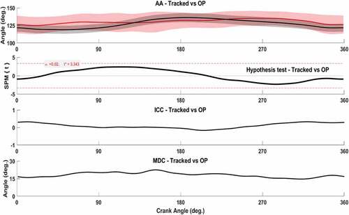
No significant differences were observed between the criterion and the OpenPose method for the ankle angle (Figure 4). Largest ICC was poor (0.32) and minimum detectable change ranged between 15–22°.

Figure 4. Upper panel shows ankle angle temporal comparison between criterion (Tracked – black) and OpenPose (OP – red). SPM 1-d statistics is shown at the second level with alpha (α) value from the Bonferroni correction indicated in dashed lines. Solid lines present the t statistic outputs from the post hoc analyses whilst the dashed red lines show the critical t value for significant differences. Intraclass correlation coefficients (ICC) across the crank cycle are shown in the third level and minimum detectable change is shown at the fourth level.

No significant differences were observed between the criterion and the OpenPose method for the knee angle (Figure 4). Largest ICC was poor (0.32) and minimum detectable change ranged between 15–22°.

Bland and Altman’s analyses indicated that the MSRA presented larger bias and wider confidence intervals than the criterion for the mean hip angle (bias = 6°; 95%CI = −16°;30°) and mean knee angle (bias = −2°; 95%CI = −41°;36°), as shown in Figure 5. OpenPose presented lower bias and tighter confidence intervals than the criterion for the mean hip angle (bias = 1°; 95%CI = −4°;7°) and mean knee angle (bias = <-1°; 95%CI = −7°;6°), as shown in Figure 5. MSRA presented larger bias and wider confidence intervals than the criterion for the hip angle range of motion (bias = −14°; 95%CI = −62°;35°) and knee angle range of motion (bias = −6°; 95%CI = −57°;45°), as shown in Figure 6. OpenPose presented lower bias and tighter confidence intervals than the criterion for the hip angle range of motion (bias = <1°; 95%CI = −12°;12°) and knee angle range of motion (bias = 3°; 95%CI = −13°;19°), as shown in Figure 6. For mean ankle angle, OpenPose presented a mean bias of −3° and 95%CI between 16° and 23°, as shown in Figure 7. For ankle range of motion, OpenPose presented a mean bias of −8° and 95%CI between −38° and 22°. Mean and standard deviation data for all methods is presented in Table 1.

Figure 5. Bland and Altman plots illustrating the mean bias (central dashed lines) and 95% confidence intervals (upper and lower dashed lines) for the mean hip and knee angles comparing the criterion (Tracked) to the MSRA and the OpenPose (OP) methods.

Figure 6. Bland and Altman plots illustrating the mean bias (central dashed lines) and 95% confidence intervals (upper and lower dashed lines) for the hip and knee ranges of motion (ROM) comparing the criterion (Tracked) to the MSRA and the OpenPose (OP) methods.

Figure 7. Bland and Altman plots illustrating the mean bias (central dashed lines) and 95% confidence intervals (upper and lower dashed lines) for the mean and range of motion (ROM) for the ankle joint comparing the criterion (Tracked) to the OpenPose (OP) method.

Table 1. Means and standard deviations for mean angle and ranges of motion (ROM) for the hip, knee and ankle joints obtained from the tracked, MSRA and OpenPose (OP) methods.

	Mean Angle			ROM
	Tracked	MSRA	OP	Tracked	MSRA	OP
Hip angle (°)	42 ±3	35 ±12	41 ±4	40 ±3	54 ±24	40 ±5
Knee angle (°)	75 ±2	77 ±19	75 ±3	69 ±5	75 ±23	66 ±10
Ankle angle (°)	127 ±5	N/A	130 ±9	19 ±6	N/A	27 ±15

Note: N/A indicates that data has not been calculated for this method.

Discussion

Data from this study demonstrates that the OpenPose method presented stronger agreement than the MSRA method to calculate angles during cycling. From analysis of the minimum detectable change, angles were consistently similar between the OpenPose and the criterion (i.e., differences of 4–8°) for the hip and knee joint angles. This finding partially supports our hypothesis because only the OpenPose presented moderate to poor agreement in relation to the criterion measure for the hip and knee joints but not for the ankle joint.

Performance of marker-less systems has been shown to vary between<1° (Ong et al., 2017) and 9° (Ota et al., 2021), which is comparable to findings from the current study. These findings are new because no prior study has analysed waveforms from cycling exercise using two-dimensional video analysis to examine the validity of marker-less methods, which provides a broader application to clinical setting and bicycle fitting than three-dimensional analysis. Even though no significant differences were observed for the MSRA or the OpenPose in relation to the criterion, the OpenPose produced greater similarity in relation to the criterion. This is evident from the smaller MDC for OpenPose, particularly for the hip and knee joints. For the ankle joint, the OpenPose method demonstrated lower performance in comparison to the hip and knee. Visual inspection of the videos generated by the OpenPose (supplementary materials) suggests that the identification of the toes was not always consistent, which likely increased the variability of the ankle joint. We can speculate that this was potentially due to increased blur at the foot from lower frame rate, which challenged OpenPose in accurately detecting the toes. An increased frame rate and image resolution should improve the accuracy of OpenPose.

Applications from using a marker-less method could range from assessing changes in motion when cyclists increase exercise intensity, change cadence or develop fatigue. As an example, ankle range of motion increases by~4° and mean ankle angle reduces by~3° when intensity is increased during cycling (R. R. Bini & Diefenthaeler, 2010). Looking at bias and 95%CI for mean angles and ranges of motion from our study suggests that OpenPose may be limited in determining these changes. Another example of implications from errors associated with the use of marker-less methods involves musculoskeletal modelling (e.g., OpenCap – Musculoskeletal forces from smartphone videos.). Simulating changes in mean knee angle of<3° in terms of the moment-arm of the vastus lateralis in a public available model (Catelli et al., 2019) would result in errors of<0.14 cm, which could be deemed small. However, due to poor to moderate agreement in relation to the criterion, further research is required to fully determine the magnitude of these errors in terms of internal loads. Implications for bicycle fitting can also be explored. The first is that, most studies recommend a range of knee angles to optimize saddle position (e.g., 30–40°.; Millour et al., 2019), which would be measurable only using OpenPose. In addition, knee forces were not sensitive to changes in knee angle of~10–14° (R. R. Bini & Hume, 2014), which suggests that large changes in cycling kinematics could be detectable particularly by the OpenPose method.

Both marker-less methods have not been extensively pre-trained using cycling images or poses taken purely from the sagittal plane. In addition, the MRSA network has been trained to analyse images with a resolution of 256 × 192 pixels whilst the OpenPose network used the whole image (i.e., 640 × 480 of frame resolution). Therefore, OpenPose had increased resolution at each frame to determine joint keypoints, potentially explaining its better accuracy. According to Cao et al. (2021), the MSRA method outperformed the OpenPose by 12.3%ual points, considering the test set of the COCO dataset. This finding contrasts with our study suggesting that it would be beneficial to undertake future training of neural networks using cycling related images. This is particularly important for the foot markers given larger discrepancies were observed in relation to the criterion. It is possible that refining the OpenPose model re-training the network to better identify the foot landmarks would improve the accuracy of the ankle joint angles. From an injury prevention perspective, cyclists with knee pain have been shown to present with~5° greater ankle dorsi-flexion (Bailey et al., 2003), which may not be detectable from OpenPose without refinements in the neural network. It is also unclear if the bicycle creates an artefact for the CNN to appropriately determine body segments, which may need further investigation.

This study had limitations, including the use of two-dimensional motion analysis, which is subject to parallax errors. The choice for using a two-dimensional model was based on a larger uptake of this method by most clinicians and bike fitters. It is important though to assume that there would be ~ 2.2–10° of error in relation to the true movement of cyclists detected using three-dimensional data (Fonda et al., 2014; García-López & Del Blanco, 2017; Umberger & Martin, 2001). However, this error should be systematic across the three methods without an influence in the comparison between the criterion and the marker-less methods. Our choice for using standard frame rate (i.e., 30 fps) was also in line with the fact that most lower cost cameras are limited in terms of frame rate, particularly those built-in Android devices. Results from OpenPose and MRSA may improve if frame rate and image resolution are higher than the currently used in this study. In addition, intra- and inter-session reproducibility should also be explored in future research to inform minimum detectable changes using marker-less methods. It is possible that the use of Bonferroni corrections may have hindered the detection of true differences between methods as this correction is conservative. Supplementing this analysis with ICCs and MDCs should have provided further clarity on whether agreement was appropriate or not with the criterion method.

In summary, the OpenPose method presented increased accuracy in determining joint angles compared to the MSRA method. Poor correlation though was observed for the ankle joint, which limits the accuracy of OpenPose to track this joint using standard video footage.

IRB Approval

HEC19001

Acknowledgments

Authors acknowledge all cyclists who took part in this study and, grant #2019/17729-0, São Paulo Research Foundation (FAPESP).

Disclosure statement

No potential conflict of interest was reported by the authors.

Additional information

Funding

Grant #2019/17729-0, São Paulo Research Foundation (FAPESP) and CNPq (grants #401004/2022-8 and 200290/2022-3)

References

- Bailey, M. P., Maillardet, F. J., & Messenger, N. (2003). Kinematics of cycling in relation to anterior knee pain and patellar tendinitis. Journal of Sports Sciences, 21(8), 649–657. https://doi.org/10.1080/0264041031000102015
- Bini, R. R., Dagnese, F., Rocha, E., Silveira, M. C., Carpes, F. P., & Mota, C. B. (2016). Three-dimensional kinematics of competitive and recreational cyclists across different workloads during cycling. European Journal of Sport Science, 16(5), 553–559. https://doi.org/10.1080/17461391.2015.1135984
- Bini, R. R., & Diefenthaeler, F. (2010). Kinetics and kinematics analysis of incremental cycling to exhaustion. Sports Biomechanics, 9(4), 223–235. https://doi.org/10.1080/14763141.2010.540672
- Bini, R. R., Diefenthaeler, F., & Mota, C. B. (2010). Fatigue effects on the coordinative pattern during cycling: Kinetics and kinematics evaluation. Journal of Electromyography and Kinesiology, 20(1), 102–107. https://doi.org/10.1016/j.jelekin.2008.10.003
- Bini, R. R., & Hume, P. A. (2014). Effects of saddle height on knee forces of recreational cyclists with and without knee pain. International SportMed Journal, 15(2), 188–199. https://www.researchgate.net/publication/263587378_EFFECTS_OF_SADDLE_HEIGHT_ON_KNEE_FORCES_OF_RECREATIONAL_CYCLISTS_WITH_AND_WITHOUT_KNEE_PAIN
- Bini, R. R., Hume, P. A., & Croft, J. L. (2011). Effects of bicycle saddle height on knee injury risk and cycling performance. Sports Medicine, 41(6), 463–476. https://doi.org/10.2165/11588740-000000000-00000
- Bini, R. R., Hume, P. A., & Kilding, A. E. (2014). Saddle height effects on pedal forces, joint mechanical work and kinematics of cyclists and triathletes. European Journal of Sport Science, 14(1), 44–52. https://doi.org/10.1080/17461391.2012.725105
- Bini, R., & Priego-Quesada, J. (in press). Methods to determine saddle height in cycling and implications of changes in saddle height in performance and injury risk: A systematic review. Journal of Sports Sciences. https://doi.org/10.1080/02640414.2021.1994727
- Bini, R. R., Rossato, M., Diefenthaeler, F., Carpes, F. P., Dos Reis, D. C., & Moro, A. R. P. (2010). Pedaling cadence effects on joint mechanical work during cycling. Isokinetics and Exercise Science, 18(1), 7–13. https://doi.org/10.3233/IES-2010-0361
- Bini, R. R., Senger, D., Lanferdini, F. J., & Lopes, A. L. (2012). Joint kinematics assessment during cycling incremental test to exhaustion. Isokinetics and Exercise Science, 20(1), 99–105. https://doi.org/10.3233/IES-2012-0447
- Bini, R. R., Serrancoli, G., Santiago, P. R. P., Pinto, A., & Moura, F. (2022). Validity of neural networks to determine body position on the bicycle. Research Quarterly for Exercise and Sport, 1–8. https://doi.org/10.1080/02701367.2022.2070103
- Burnie, L., Barratt, P., Davids, K., Worsfold, P., & Wheat, J. (2020). Biomechanical measures of short-term maximal cycling on an ergometer: A test-retest study. Sports Biomechanics, 1–19. https://doi.org/10.1080/14763141.2020.1773916
- Cao, Z., Hidalgo, G., Simon, T., Wei, S. E., & Sheikh, Y. (2021). OpenPose: Realtime multi-person 2D pose estimation using part affinity fields. IEEE Transactions on Pattern Analysis and Machine Intelligence, 43(1), 172–186. https://doi.org/10.1109/TPAMI.2019.2929257
- Catelli, D. S., Wesseling, M., Jonkers, I., & Lamontagne, M. (2019). A musculoskeletal model customized for squatting task. Computer Methods in Biomechanics and Biomedical Engineering, 22(1), 21–24. https://doi.org/10.1080/10255842.2018.1523396
- D’antonio, E., Taborri, J., Mileti, I., Rossi, S., & Patané, F. (2021). Validation of a 3D markerless system for gait analysis based on openpose and two RGB webcams. IEEE Sensors Journal, 21(15), 17064–17075. https://doi.org/10.1109/JSEN.2021.3081188
- Drazan, J. F., Phillips, W. T., Seethapathi, N., Hullfish, T. J., & Baxter, J. R. (2021). Moving outside the lab: Markerless motion capture accurately quantifies sagittal plane kinematics during the vertical jump. Journal of Biomechanics, 125, 110547. https://doi.org/10.1016/j.jbiomech.2021.110547
- Faul, F., Erdfelder, E., Lang, A. -G., & Buchner, A. (2007). G*power 3: A flexible statistical power analysis program for the social, behavioral, and biomedical sciences. Behavior Research Methods, 39(2), 175–191. https://doi.org/10.3758/BF03193146
- Ferrer-Roca, V., Bescós, R., Roig, A., Galilea, P., Valero, O., & García-López, J. (2014). Acute Effects of small changes in bicycle saddle height on gross efficiency and lower limb kinematics. Journal of Strength and Conditioning Research. 28(3), 784–791. https://doi.org/10.1519/JSC.0b013e3182a1f1a9
- Fonda, B., Sarabon, N., & Li, F. -X. (2014). Validity and reliability of different kinematics methods used for bike fitting. Journal of Sports Sciences, 32(10), 940–946. https://doi.org/10.1080/02640414.2013.868919
- García-López, J., & Del Blanco, P. A. (2017). Kinematic analysis of bicycle pedalling using 2d and 3d motion capture systems. ISBS Proceedings Archive, 35(1), 125.
- Holliday, W., & Swart, J. (2021). A dynamic approach to cycling biomechanics. Physical Medicine and Rehabilitation Clinics of North America, 33(1), 1–13. https://doi.org/10.1016/j.pmr.2021.08.001
- Holliday, W., Theo, R., Fisher, J., & Swart, J. (2019). Cycling: Joint kinematics and muscle activity during differing intensities. Sports Biomechanics, 1–15. https://doi.org/10.1080/14763141.2019.1640279
- Johnson, C. D., Outerleys, J., & Davis, I. S. (2022). Agreement between sagittal foot and tibia angles during running derived from an open-source markerless motion capture platform and manual digitization. Journal of Applied Biomechanics, 38(2), 1–6. https://doi.org/10.1123/jab.2021-0323
- Koo, T. K., & Li, M. Y. (2016). A guideline of selecting and reporting intraclass correlation coefficients for reliability research. Journal of Chiropractic Medicine, 15(2), 155–163. https://doi.org/10.1016/j.jcm.2016.02.012
- Lin, T. Y., Maire, M., Belongie, S., Hays, J., Perona, P., Ramanan, D., Zitnick, C. L., Zitnick, C. L. (2014). Microsoft COCO: Common objects in context. Paper presented at the Computer Vision – ECCV 2014,
- Millour, G., Duc, S., Puel, F., & Bertucci, W. (2019). Comparison of static and dynamic methods based on knee kinematics to determineoptimal saddle height in cycling. Acta of Bioengineering and Biomechanics / Wroclaw University of Technology, 21(4), 93–99. https://doi.org/10.37190/ABB-01428-2019-02
- Needham, L., Evans, M., Cosker, D. P., Wade, L., McGuigan, P. M., Bilzon, J. L., & Colyer, S. L. (2021). The accuracy of several pose estimation methods for 3D joint centre localisation. Scientific Reports, 11(1), 1–11. https://doi.org/10.1038/s41598-021-00212-x
- Ong, A., Harris, I. S., & Hamill, J. (2017). The efficacy of a video-based marker-less tracking system for gait analysis. Computer Methods in Biomechanics and Biomedical Engineering, 20(10), 1089–1095. https://doi.org/10.1080/10255842.2017.1334768
- Ota, M., Tateuchi, H., Hashiguchi, T., & Ichihashi, N. (2021). Verification of validity of gait analysis systems during treadmill walking and running using human pose tracking algorithm. Gait & Posture, 85, 290–297. https://doi.org/10.1016/j.gaitpost.2021.02.006
- Ota, M., Tateuchi, H., Hashiguchi, T., Kato, T., Ogino, Y., Yamagata, M., & Ichihashi, N. (2020). Verification of reliability and validity of motion analysis systems during bilateral squat using human pose tracking algorithm. Gait & Posture, 80, 62–67. https://doi.org/10.1016/j.gaitpost.2020.05.027
- Pagnon, D., Domalain, M., & Reveret, L. (2022). Pose2sim: An End-to-end workflow for 3D markerless sports kinematics—Part 2: Accuracy. Sensors, 22(7), 2712. Retrieved from, https://www.mdpi.com/1424-8220/22/7/2712
- Pataky, T. C., Robinson, M. A., & Vanrenterghem, J. (2013). Vector field statistical analysis of kinematic and force trajectories. Journal of Biomechanics, 46(14), 2394–2401. https://doi.org/10.1016/j.jbiomech.2013.07.031
- Robinson, M. A., Vanrenterghem, J., & Pataky, T. C. (2021). Sample size estimation for biomechanical waveforms: Current practice, recommendations and a comparison to discrete power analysis. Journal of Biomechanics, 122, 110451. https://doi.org/10.1016/j.jbiomech.2021.110451
- Sayers, M. G. L., & Tweddle, A. L. (2012). Thorax and pelvis kinematics change during sustained cycling. International Journal of Sports Medicine, 33(4), 314–319. https://doi.org/10.1055/s-0031-1291363
- Serrancolí, G., Bogatikov, P., Huix, J. P., Barberà, A. F., Egea, A. J. S., Ribé, J. T., Susín, A. … Susín, A. (2020). Marker-less monitoring protocol to analyze biomechanical joint metrics during pedaling. IEEE Access, 8, 122782–122790. https://doi.org/10.1109/ACCESS.2020.3006423
- Suriyaamarit, D., & Boonyong, S. (2018). Reliability and minimal detectable change of sit-to-stand kinematics and kinetics in typical children. Human Movement, 19(3), 48–54. https://doi.org/10.5114/hm.2018.76079
- Swart, J., & Holliday, W. (2019). Cycling biomechanics optimization—the (R) evolution of bicycle fitting. Current Sports Medicine Reports, 18(12), Retrieved from https://journals.lww.com/acsm-csmr/Fulltext/2019/12000/Cycling_Biomechanics_Optimization_the__R_.13.aspx.
- Szczerbik, E., & Kalinowska, M. (2011). The influence of knee marker placement error on evaluation of gait kinematic parameters. Acta of Bioengineering and Biomechanics / Wroclaw University of Technology, 13(3), 43–46.
- Umberger, B. R., & Martin, P. E. (2001). Testing the planar assumption during ergometer cycling. Journal of Applied Biomechanics, 17(1), 55–62. https://doi.org/10.1123/jab.17.1.55
- Xiao, B., Wu, H., & Wei, Y. (2018). Simple baselines for human pose estimation and tracking. Paper presented at the Computer Vision – ECCV 2018,