A Bayesian hierarchical diffusion model decomposition of performance in Approach–Avoidance Tasks

Abstract

Common methods for analysing response time (RT) tasks, frequently used across different disciplines of psychology, suffer from a number of limitations such as the failure to directly measure the underlying latent processes of interest and the inability to take into account the uncertainty associated with each individual's point estimate of performance. Here, we discuss a Bayesian hierarchical diffusion model and apply it to RT data. This model allows researchers to decompose performance into meaningful psychological processes and to account optimally for individual differences and commonalities, even with relatively sparse data. We highlight the advantages of the Bayesian hierarchical diffusion model decomposition by applying it to performance on Approach–Avoidance Tasks, widely used in the emotion and psychopathology literature. Model fits for two experimental data-sets demonstrate that the model performs well. The Bayesian hierarchical diffusion model overcomes important limitations of current analysis procedures and provides deeper insight in latent psychological processes of interest.

Keywords:

• Response time task
• Action tendencies
• Individual differences
• Latent psychological processes
• Emotion
• Psychopathology

We would like to thank Dr Dinska Van Gucht for providing us with her data-set and Dr Josine Verhagen for her help with the Bayesian ANOVA.

This research was supported by an Innovation Scheme (Vidi) Grant [452-09-001] of the Netherlands Organisation for Scientific Research (NWO) awarded to Tom Beckers and a consolidator grant from the European Research Council (ERC) [283876] awarded to Eric-Jan Wagenmakers. Merel Kindt is funded by a Vici grant [453-07-006] from NWO. Angelos-Miltiadis Krypotos is a scholar of the Alexander S. Onassis Public Benefit Foundation [FZE 039/2011-2012].

Conclusions about latent psychological processes are often based on performance in so-called speeded response time (RT) tasks, where participants are put under pressure to respond to a stimulus quickly and the main dependent variable is response latency. For instance, tasks such as the emotional Stroop task (Stroop, 1935; Williams, Mathews, & MacLeod, 1996), the dot-probe task (MacLeod, Mathews, & Tata, 1986; Salemink, van den Hout, & Kindt, 2007), the implicit association test (IAT; Greenwald, McGhee, & Schwartz, 1998) and the Approach–Avoidance Task (AAT; De Houwer, Crombez, Baeyens, & Hermans, 2001; Krieglmeyer & Deutsch, 2010) are commonly used in psychology in order to measure and understand putative latent processes such as cognitive and attentional biases, implicit memory associations and implicit attitudes or action tendencies.

Despite their substantial contribution to the literature, and despite their empirical popularity, most RT tasks suffer from an important limitation. This limitation concerns the suboptimal analysis strategies that are employed to draw substantive conclusions from the observed data. Specifically, the standard methods of analysis do not directly measure the psychological processes of interest, that is, they use a general statistical model instead of a cognitive process model. Moreover, the variability or uncertainty involved in an individual's data is ignored by the consideration of a single-point estimate (e.g., mean or median) per individual.

The aim of the present paper is to demonstrate how the above limitations can be overcome by a cutting-edge analysis technique known as a Bayesian hierarchical diffusion model decomposition. This technique is applicable to the analysis of RT tasks generally, but we illustrate its use here for the AAT, a task that is widely used to measure implicit action tendencies in experimental psychopathology research (e.g., Rinck & Becker, 2007; Spruyt et al., 2013).

The outline of this paper is as follows. We first describe the theoretical foundations of AATs. Second, we describe common AAT data analysis techniques and their limitations. Next, we present Ratcliff's diffusion model (Ratcliff, 1978; Ratcliff & McKoon, 2008) and outline its implementation in a Bayesian hierarchical framework. We then present two experimental data-sets: the first one concerning avoidance tendencies—which are mainly studied in anxiety disorders and phobias—and the second data-set concerning approach tendencies—which are mainly of interest in the addiction literature. Throughout, we compare the outcome of traditional analytic techniques to the outcome of our diffusion model decomposition. We conclude by summarising our results and commenting on the generality of the new analysis technique and the benefits and challenges that it brings.

APPROACH–AVOIDANCE REACTION TIME TASKS

People have the inherent tendency to approach rewarding stimuli and avoid potential dangers (i.e., Thorndike's “law of effect”, see Chance, 1999). People, for example, tend to approach food when hungry but will recoil from a car heading their way. Various psychological theories conceptualise these action tendencies as vital emotional reactions, with positive valence cues automatically triggering approach responses and negative valence cues automatically triggering avoidance reactions (Bradley & Lang, 2007; Frijda, 1988; Lang & Bradley, 2008; Rutherford & Lindell, 2011). Some theories even posit that emotions may be best defined as action tendencies (Frijda, 1988; Lang, 1985).

A common way to identify and measure action tendencies is via AATs. Although different versions of AAT exist (Krieglmeyer & Deutsch, 2010), participants are typically instructed to symbolically approach and avoid categories of stimuli that differ in their emotional valence; the critical assumption is that RTs are influenced both by the valence of the stimulus (i.e., appetitive vs. aversive) and by the response assignment (approach vs. avoidance). For instance, participants in De Houwer et al.'s (2001) study had to manoeuvre a virtual manikin towards and away from positively and negatively valence words. Results confirmed the expected interaction between stimulus valence and response assignment: participants responded faster when they had to make the manikin approach words with positive valence or when they had to make it avoid words with negative valence than vice versa. In a similar vein, Rinck and Becker (2007) instructed spider-fearful individuals and non-anxious individuals to respond to pictures by pushing (avoidance) or pulling (approach) a joystick. In the first block of trials, half of the participants had to push the joystick in response to pictures depicting spider stimuli and pull the joystick in response to pictures showing neutral stimuli, with the other half of the participants doing the opposite. Instructions were reversed for the second block. The results showed that—compared to the control participants and compared to the neutral pictures—the spider-fearful participants were quicker to respond to the spider pictures when they had to push than when they had to pull. Similar AATs have been used with a diversity of stimuli, including alcohol (Spruyt et al., 2013; Wiers, Eberl, Rinck, Becker, & Lindenmeyer, 2011; Wiers, Rinck, Kordts, Houben, & Strack, 2010), cannabis (Cousijn, Goudriaan, & Wiers, 2011), social groups (Neumann, Hülsenbeck, & Seibt, 2004), facial expressions (Heuer, Rinck, & Becker, 2007), conditioned appetitive cues (Van Gucht, Vansteenwegen, van den Bergh, & Beckers, 2008) and conditioned fear cues (Krypotos, Effting, Arnaudova, Kindt, & Beckers, 2014).

Although widely used across social and clinical psychology, no consensus has been reached on how to best analyse AATs statistically. After reviewing the published literature, we found divergence in analytic techniques as regards (1) the normalisation of the RT distributions, (2) the estimation of central tendency, (3) the handling of error responses and (4) the computation of an approach–avoidance tendencies index. At the same time, there is consensus regarding other data analysis strategies such as the collapsing of data across participants. Regardless of the degree of consensus, all current methods of analysis have serious limitations: RTs and error rates are not accounted for in a common framework; the psychological process of interest is not estimated directly; the shape of the RT distribution (for correct and error responses) is left unaccounted for; and the calculation of a single-point estimate per individual ignores variability and implies a considerable loss of information. These limitations constrain the substantive conclusions that can be drawn from AAT data. Increasing the validity of the conclusions derived from AAT data is timely given that AATs are increasingly applied in intervention research. Specifically, variations of the AAT tasks are currently being applied to clinical populations (e.g., in alcohol addicts) as a way to change dysfunctional action tendencies (i.e., excessive approach towards alcohol stimuli in the study of Wiers et al., 2011). Since decisive conclusions as to whether action tendencies have been successfully modified are based on the AAT data, a more accurate estimation of AAT performance will allow more solid conclusions regarding the success or failure of action tendency modification.

COMMON ANALYSIS TECHNIQUES FOR AAT DATA

In this section, we summarise the common analysis strategies for AAT data. We accompany each strategy with examples from the literature on the use of AAT in emotion or psychopathology research along with our considerations.

Normalisation of the RT distribution

RTs are positively skewed and this complicates their statistical analysis (Heathcote, Popiel, & Mewhort, 1991). Consequently, researchers follow several strategies for data normalisation. The two most common strategies applied to the RTs of each individual are outlier removal (Ratcliff, 1993) and data transformation (Mead, 1990). For outlier removal, different cut-off points are used which can either be fixed (e.g., RTs longer than 3000 ms in Van Gucht et al., 2008) or variable (e.g., top and bottom 1% of RT distribution in Vrijsen, van Oostrom, Speckens, Becker, & Rinck, 2013; or RTs deviating more than two standard deviations from the mean in Klein, Becker, & Rinck, 2011). For data transformation, the log transformation is the most popular (e.g., in Adams, Ambady, Macrae, & Kleck, 2006 and in Chen & Bargh, 1999).

When used jointly, these approaches result in RT distributions that are (almost) normal. However, outlier removal for skewed distributions is by definition problematic: it can be difficult to tell whether an extremely long RT is due to an attentional lapse or whether it is a valid sample from a right-skewed distribution (Heathcote et al., 1991). Rather than transforming data so that they meet the requirements of standard statistical tests, it may be better to use statistical models that are valid for the kind of skewness that is present in RT data.

Estimation of central tendency

There is some debate on what measure of central tendency best summarises RTs for each stimulus–response condition. The most common choices are the mean (e.g., in De Houwer et al., 2001) and the median (e.g., in Rinck & Becker, 2007). The median RT arguably provides a better summary statistic (Hays, 1973) because it is less influenced by outlying values compared to the mean (but see Miller, 1988, for counter arguments). The main problem with measures of central tendency is that they summarise an entire RT distribution using a single number, which implies a considerable loss of information (McAuley, Yap, Christ, & White, 2006).

Error responses

In the statistical analyses of AATs, error responses are typically ignored (e.g., in Van Gucht et al., 2008) or taken into account separately, by conducting additional statistical tests with proportion of errors as the new dependent variable (e.g., in De Houwer et al., 2001). Both approaches can yield misleading results. Ignoring error responses results in a loss of information and can blind the researcher to the signature finding of a speed–accuracy trade-off, where faster responses can be obtained at the cost of making more errors (Pachella, 1974; Schouten & Bekker, 1967). Conducting separate tests for RT and accuracy similarly fails, as it does not acknowledge the intimate connection between these two measures of performance (e.g., Wagenmakers, van der Maas, & Grasman, 2007). These drawbacks are exacerbated by the fact that the speed–accuracy trade-off is non-linear, such that an increase in accuracy of a few percentage points may correspond to a decrease in mean RT of hundreds of milliseconds (e.g., Ratcliff & McKoon, 2008).

Ignoring within-subjects uncertainty

In most AAT studies, the mean or median RTs (e.g., in De Houwer et al., 2001; Van Gucht et al., 2008; Wiers, Rinck, Dictus, & Van den Wildenberg, 2009) of each participant are included in the statistical analyses. Importantly, such an approach, in which only one value per participant is retained, implies that the individuals' RTs are known with absolute accuracy (i.e., without any statistical noise), which is hardly the case in sparse data-sets, such as those in many applications in clinical psychology. In view of this difficulty in individual data averaging, it could be argued that analysing each participant separately would be more accurate. However, such an approach would hinder the valid generalisation of the results to the population.

Computation of an AAT index

After the computation of central tendencies for the different types of trials, researchers typically calculate an approach–avoidance tendencies index that represents the relative strength of the corresponding action tendencies. Strategies for calculating this index include (1) taking the difference between the mean RTs for congruent trials (i.e., approach positive valence stimuli and avoid negative valence stimuli) and for incongruent trials (i.e., avoid positive valence and approach negative valence), as in De Houwer et al., 2001; (2) taking the difference of the differences between approach and avoidance trials for each type of stimulus (e.g., in Wiers et al., 2010); and (3) assessing approach and avoidance tendencies separately for each stimulus category (e.g., in Voncken, Rinck, Deckers, & Lange, 2011).

To illustrate the differences of the above computational strategies, we present a hypothetical example in which an experimenter has collected approach–avoidance RT data in response to picture stimuli with positive or negative valence. We generated data from an ex-Gaussian distribution that generally fits RT data well (Ratcliff, 1979), for each stimulus–response category for one participant (see Table 1 and online Supplementary material). According to the first strategy, we compute the AAT index by following three steps: (1) take the mean RT of the congruent trials, in this example the approach positive and avoid negative conditions, (2) take the mean RT of the incongruent trials, in this example the approach negative and avoid positive conditions, and (3) subtract the incongruent from the congruent trials. In our simulated data-set, this results in an AAT index of –167 ms. According to the second strategy, we compute the AAT index as follows: (1) compute the mean RT for each stimulus–response category—in this example the combinations are: (i) approach speed for positive pictures, (ii) approach speed for negative pictures, (iii) avoidance speed for positive pictures and (iv) avoidance speed for negative pictures—and (2) for each stimulus category separately, subtract the avoidance responses from the approach responses. In our example, for the positive valence stimuli, we should subtract the mean RT of the avoid positive picture condition from the approach positive picture condition and similarly for the negative stimuli. The third step, (3), would be to compute the difference between the two resulting numbers. In our example, this resulted in an AAT index of –333 ms. The third and final strategy entails the first two steps of the second strategy. In our data-set, this resulted in a value of –307.07 ms for positive stimuli, and a value of 26.01 ms for the negative stimuli.

Table 1. Example mean RTs (in ms) for each stimulus (i.e., positive vs. negative) by response (i.e., approach vs. avoidance) combination of our hypothetical in-text experiment

Approach positive valence picture	Approach negative valence picture	Avoid positive valence picture	Avoid negative valence picture
747.20	1054.27	777.08	751.07

The example above shows that even with the same data, the resulting AAT index differs according to the selected computational strategy. More importantly still, although one could debate the merits and drawbacks of each approach, and although in practice all strategies may lead to similar conclusions, a core problem across the different strategies as they are typically used is that they collapse across different RT distributions. As such, they may lead to inaccurate AAT estimations. Moreover, by computing the difference between two quantities that have been averaged across participants and across trials, the index of action tendencies is necessarily coarse.

Psychological processes involved in decision-making

Like any other decision-making task in which participants have to choose quickly between alternative responses, AAT performance recruits basic cognitive processes such as the speed of information accumulation, bias, motor execution time and response caution. In other tasks, these processes have been quantified using the diffusion model (Ratcliff, 1978; Wagenmakers, 2009), one of the most prominent process models in experimental psychology and neuroscience. AAT data have not yet been analysed using the diffusion model. It is therefore an open issue whether the model can provide an adequate account of the data.

Summary

To sum up, the current data analysis strategies employed in the AAT literature suffer from substantial shortcomings stemming from (1) their need for normally distributed data, while RT distributions are often skewed; (2) the disregard of error trials which can result in loss of information; (3) the non-consideration of the speed–accuracy trade-off, where faster responses are obtained in sacrifice of accuracy; (4) the computation of an approach–avoidance tendencies index that is relatively coarse, as its computation is typically based on the collapsing of different RT distributions; (5) the non-consideration of within-subjects uncertainty; and (6) the neglect of latent psychological processes involved in the AAT.

BAYESIAN HIERARCHICAL DIFFUSION Modelling

This section outlines a statistical process model approach that aims to overcome the shortcomings discussed above. We first describe the diffusion model and then present the advantages of the hierarchical Bayesian framework that we use to estimate the model's parameters.

The diffusion model

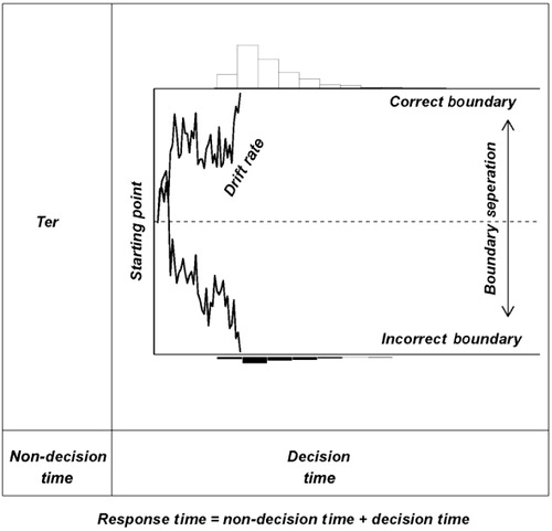
The Ratcliff diffusion model (e.g., Ratcliff, 1978; Ratcliff & McKoon, 2008; Smith & Ratcliff, in press; Wagenmakers, 2009) conceptualises the decision process as the interplay between different psychological processes that are each represented by a separate model parameter. According to the model, every binary decision process starts at z, a parameter reflecting the a-priori bias towards the upper or lower boundary (representing one or the other decision). The decision process itself consists of the gradual accumulation of noisy information, a process whose efficiency is reflected in drift rate v. High absolute drift rates generate decisions that are fast and accurate; slow absolute drift rates (i.e., drift rates near zero) generate decisions that are slow and error-prone. Information accumulation continues until an upper or lower boundary is reached and a decision is initiated. Boundary separation a represents response caution and hence quantifies the speed–accuracy trade-off. High values of boundary separation result in accurate but long RTs, and low values of boundary separation result in short but error-prone RTs. The final parameter, non-decision time Ter, captures everything that precedes or follows the decision process, such as stimulus encoding and response execution (Luce, 1986). Although extensions of the diffusion model (Ratcliff & Tuerlinckx, 2002) account for across trial variability in drift rate, starting point and non-decision time, we limit ourselves here to the four main parameters.¹

In sum, the major components of the diffusion model (see Figure 1) are: (1) drift rate, v; (2) boundary separation, a; (3) starting point, z; and (4) non-decision time, T_er.

Figure 1. Graphical representation of the diffusion model (Ratcliff & McKoon, 2008). Following stimulus presentation (not shown), noisy information is accumulated until reaching the upper boundary—associated with the correct response—or the lower boundary—associated with the incorrect response—following which a response is initiated. Observed RTs are the sum result of decision time and non-decision time: decision time reflects the duration of the information accumulation process, whereas non-decision time reflects the duration of non-specific processes such as stimulus encoding and response execution.

The diffusion model naturally accounts for a number of benchmark findings (Ratcliff, 2002), including the right-skew of RT distributions, the speed–accuracy trade-off, the linear relation between RT mean and RT standard deviation (Wagenmakers & Brown, 2007), the relative speed of errors as a function of bias and the fact that the right-skew increases with difficulty. Because the model parameters are associated with specific cognitive processes, fitting the diffusion model to data allows for an informative decomposition of performance (e.g., Dutilh, Krypotos, & Wagenmakers, 2011; Leite & Ratcliff, 2011; Mulder, Wagenmakers, Ratcliff, Boekel, & Forstmann, 2012; van Ravenzwaaij, Dutilh, & Wagenmakers, 2012). In sum, a diffusion model decomposition allows for a more detailed and informative summary of performance than can be achieved by most standard statistical analysis techniques for AATs. Of importance, variants of the diffusion model have recently led to increases in understanding regarding emotion effects (e.g., see Pe, Vandekerckhove, & Kuppens, 2013) and psychopathology (e.g., see Ho et al., 2014; Strauss et al., 2011; White, Ratcliff, Vasey, & McKoon, 2010a, 2010b).

Bayesian hierarchical modelling

As mentioned before, a common approach in the analysis of AATs is to collapse data across trials and participants, and to estimate the grand means for each combination of stimulus and response assignment. This nomothetic approach (Kristjansson, Kircher, & Webb, 2007) assumes that the mean responses are valid representations of individuals' scores, with any within-group differences treated as statistical noise. Consequently, individual differences are not taken sufficiently into account (Heathcote, Brown, & Mewhort, 2000; Ratcliff, 1979) even though these differences may be pronounced. On the other hand, the idiographic approach (Kristjansson et al., 2007) considers individual differences as systematic and reliable. In the idiographic approach, each participant is considered in isolation. With sparse data, however, this approach is prone to error (Efron & Morris, 1977).

In between the “complete pooling” approach implicit in the averaging method and the “complete independence” approach implicit in per-participant analyses lies a compromise solution known as hierarchical modelling (Rouder & Lu, 2005; Shiffrin, Lee, Kim, & Wagenmakers, 2008). This solution takes within-subject variability into account, while at the same time-assuming that participants are similar to one another, with the degree of similarity estimated from the data (e.g., Shiffrin et al., 2008). Specifically, in hierarchical models, there are two kinds of parameters: (1) group-level parameters (monothetic patterns) and (2) individual-level parameters (idiographic patterns) that are constrained by the group-level parameters (Morey, Pratte, & Rouder, 2008; Nilsson, Rieskamp, & Wagenmakers, 2011). The group-level parameters capture the extent to which the participants are similar and strength can be borrowed across participants. For instance, assume that each participant i has a drift rate v_i. Each individual drift rate may be assumed to be constrained by a group-level normal distribution with mean µ_v and variance , that is, v_i ~ N (µ_v, ). Note here, that in a hierarchical framework, the within-subject variability is taken into account, in contrast to common averaging techniques (see above). When participants are very similar to each other, σ ₂ → 0, the hierarchical approach reduces to the nomothetic approach. When participants are highly dissimilar, σ₂ >> 0, the hierarchical approach reduces to the idiographic approach. Thus, the hierarchical method tunes itself to the degree of similarity between participants and adjusts the parameter estimates accordingly. When participants are very similar, precise estimates can be obtained even with few trials per participant. This is of great benefit in situations where one has many participants but few trials per participant, as is the case in many applications in clinical psychology.

In the following, we estimated the model parameters in a Bayesian manner. This means that parameters are given prior distributions that are then updated to posterior distributions. These distributions reflect the degree of belief or degree of certainty associated with their possible values. The Bayesian framework has several theoretical advantages over classical frequentist statistics (Dienes, 2011; Lee, 2011). In addition, hierarchical models (and possible extensions) are naturally accommodated within the Bayesian framework (Dyjas, Grasman, Wetzels, van der Maas, & Wagenmakers, 2012; Lee, 2011; Lee & Wagenmakers, 2013; Rouder & Lu, 2005; Wiecki, Sofer, & Frank, 2013). Nowadays, Bayesian estimation is relatively straightforward using numerical methods such as Markov chain Monte Carlo (MCMC; Lynch, 2007).

In sum, the Bayesian hierarchical model produces posterior distributions for model parameters both on the individual level and on the group level. In general, sparse data procedures, typical in psychopathology research, suggest wide posterior distributions, reflecting high uncertainty in the parameter values. However, with many somewhat similar participants, the group variance may be estimated to be low, and this encourages the borrowing of strength across participants, sharpening and shrinking the individual estimates towards the group mean (for a frequentist discussion of the advantages of shrinkage, see Efron & Morris, 1977).

All in all, the Bayesian hierarchical diffusion model decomposition (1) does not assume normal RT distributions, (2) accounts for error trials and the speed–accuracy trade-off, (3) allows for fine-grained assessment of approach–avoidance tendencies, (4) respects individual differences and (5) estimates latent psychological processes involved in the AAT. Next, we fit our model to two experimental data-sets.

MODEL APPLICATION TO EXPERIMENTAL DATA

We applied the Bayesian hierarchical diffusion model to the data of Experiment 1 of Krypotos et al. (2014), from now on data-set 1, and Experiment 1 of Van Gucht et al. (2008), from now on data-set 2. We have selected these data-sets because they both have a limited number of trials and participants, typical for the experimental psychopathology literature. Furthermore, conditioned avoidance responses, tested in the first data-set, are particularly relevant for the anxiety disorders literature, whereas approach responses, tested in the second data-set, are of prime interest in addiction research. Both data-sets are available on request.

Experimental data-set 1

Description of experiment—data-set 1

Our participants (N = 32) first underwent a fear conditioning procedure during which a picture of a neutral stimulus (i.e., the Conditioned Stimulus or CS⁺; for instance, a cube) was paired with an electric shock, whereas another neutral stimulus (CS^–; for instance, a cylinder) was never followed by an electric shock. Each CS was presented 8 times (16 times in total). Each trial lasted 8 s, with inter-trial intervals of 15, 20 or 25 s, with a 20-s mean. In case of a CS⁺ trial, electric stimulation of 2 ms was delivered to the participant's non-preferred hand, 7.5 s after stimulus onset.

Following the conditioning procedure, participants were instructed to move a virtual manikin quickly and accurately towards and away from the presented CSs. In each trial, the manikin was presented on the top or bottom half of a black screen. After 1500 ms, a CS picture was presented on the other half of the screen. Then, participants could move the manikin up or down by pressing the “B” or the “Y” button, respectively.² Each participant contributed 32 RTs, divided equally across four categories: (1) Approach CS⁺ (incongruent), (2) Approach CS^– (congruent), (3) Avoid CS⁺ (congruent) and (4) Avoid CS⁻ (incongruent). We expected participants to be faster in the congruent trials (i.e., avoid the CS⁺ and approach the CS^–) than in the incongruent trials (i.e., approach the CS⁺ and avoid the CS^–). Our hypothesis stems from the observation that the CS⁺ stimulus evokes negative evaluations, since during the fear conditioning procedure it was paired with shock, and the CS⁻ positive evaluations, since during the fear conditioning procedure it signalled safety (i.e., absence of shock). CS evaluations were also in line with this hypothesis (see Krypotos et al., 2014).

Initial analyses—data-set 1

Repeating the original analyses for the sake of completeness, we computed median RTs for each individual and for each condition. The means of the individual medians are depicted in the top panel of Figure 2. We then performed a 2 (Stimulus Type: CS⁺ vs. CS^–) × 2 (Required Response: approach vs. avoidance) repeated measures frequentist analysis of variance (ANOVA) with Stimulus Type and Required Response as within-subjects factors.

Figure 2. Top panel: Average mean RT in ms for Experiment 1 of Krypotos et al. (2014). Error percentages for each condition are shown on top of each bar. Error bars represent standard errors of the mean. Middle panel: Kernel density estimates of the posterior distributions for the drift rate parameters of the first data-set (Krypotos et al., 2014). Note that the distributions refer to the group parameters. The left panel shows the drift rate distribution for the Avoid CS^– condition. The right panel shows the drift rate distributions for the Approach CS^–, Approach CS⁺ and Avoid CS⁺ conditions, all relative to the Avoid CS^– condition. From the results, it is apparent that (1) participants exhibited the lowest drift rate in the Avoid CS^– condition, compared to the other three conditions and (2) that the Approach CS^–, Approach CS⁺ and Avoid CS⁺ conditions highly overlap with each other. Bottom Panel: Kernel density estimate of the posterior distribution for the group drift rate AAT index for data-set 1. The posterior mass is mostly positive, suggesting that, as expected, participants accumulated information faster on congruent compared to incongruent trials.

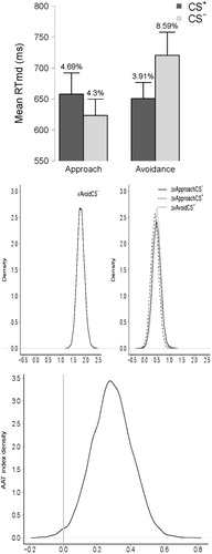
Results showed a non-significant main effect of Stimulus Type, F(1, 31) = 1.34, p = .26, = .04, and a significant main effect of Required Response, F(1, 31) = 9.33, p = .01, = .23. Of importance, the Stimulus Type × Required Response interaction was significant, F(1, 31) = 7.56, p = .01, = .20, indicating that participants were faster in approaching the CS^– and avoiding the CS⁺ than the reverse.

Given that conventional significance tests overstate the evidence against the null hypothesis (Edwards, Lindman, & Savage, 1963; Sellke, Bayarri, & Berger, 2001; Wagenmakers, 2007), we also performed a Bayesian repeated measures ANOVA (Rouder, Morey, Speckman, & Province, 2012; Wetzels, Grasman, & Wagenmakers, 2012). The key outcome of this analysis is the Bayes factor (BF), a quantity that grades the decisiveness of the evidence that the data provide for one model versus another (Jeffreys, 1961). A BF of 10, for example, indicates that the data are 10 times more likely under one model than under the other. Here, we compared a model that takes both the main effects and their interaction into account (i.e., the full model) to a model that includes only the main effects (i.e., the restricted model). The results showed that the data are almost 17 times (BF = 16.92) more likely under the full model than under the restricted model. This result is consistent with the frequentist ANOVA.

General method—data-set 1

The major challenge in fitting the model to the data is that there are only eight observations per participant per condition. Confronted with such a sparse data-set, traditional methods are simply unable to estimate the model parameters in any meaningful way. The Bayesian hierarchical implementation, however, borrows strength across participants through group-level structures, uses prior knowledge about plausible parameter values to restrict the parameter space and produces posterior distributions to indicate the uncertainty about the parameters at hand. Nevertheless, there are limits on the degree to which a sparse data-set can support the estimation of parameters in a relatively complex model. Hence we restricted the model in several ways. First, we assumed that performance differences across the four conditions were due to drift rate only. This assumption is based in part on the typical AAT trial structure in which participants have no advanced knowledge about the nature of the stimulus and the required response (approach vs. avoidance). Second, we assumed a symmetric starting point, z = a/2, so that avoid and approach responses were equally attractive a priori. Finally, we did not allow parameters a, z and T_er to vary across trials (e.g., Wagenmakers et al., 2007). Hence, our model is a measurement model in which we assumed a priori which parameters are allowed to differ across conditions. The goal of this measurement model is to offer a comprehensive and principled alternative to the less sophisticated measurement models that are currently in use. This approach is an example of “cognitive psychometrics” (Batchelder, 1998).

We estimated, for each participant i, the posterior distributions of six different parameters: four drift rates (i.e., one per condition), boundary separation and non-decision time. Since all participants contributed to all stimulus–response categories, we used a within-subjects model in which one arbitrary drift rate—here the one corresponding to the “Avoid CS⁻” condition in which the longest RTs were observed—was designated as the baseline, and the other three drift rates were estimated as differences from that baseline. Choosing any other drift rate as baseline yields identical results. We used informative priors which reflect parameter values from a meta-analysis by Matzke and Wagenmakers (2009).³

All observations for every participant were entered in our analysis. When using MCMC, it is important to ensure that the sampled values have converged from the random starting value to the posterior distribution. To assess convergence we ran three chains, each one of them consisting of 10,000 samples.³ Next, we assessed convergence by computing the R-hat (Gelman–Rubin) statistic, with values below 1.1 indicating successful convergence, and by visually inspecting the chains in order to see whether they resembled a “fat hairy caterpillar”.

Following that, we assessed the quality of the model fit by first simulating data, based on the model's parameter estimations, and by then plotting the real data against the simulated data for the .1, .3, .5 and .9 RT quantiles for each stimulus by response condition.³

We then defined a group-level “drift rate” AAT index as the difference in drift rate between the incongruent and congruent conditions. That is, we obtained a posterior distribution for the drift rate AAT index by using the group posterior distributions for the drift rate of each condition and by computing the final AAT index as follows: AAT_v = mean (Approach , Avoid )—mean (Approach , Avoid ).⁴ By defining the AAT index on the level of the latent drift rate process, we avoid ambiguity about how to average over RT distributions, we take both RT and accuracy into account and we avoid contamination from external processes such as response caution and non-decision time.

Posterior distributions—data-set 1

All R-hat values were below 1.1, indicating successful convergence for all chains. Furthermore, we visually inspected the chains and confirmed that they resembled a “fat hairy caterpillar”.⁵ The simulated data fit the real data quite well (see online Supplementary material).

The middle panel of Figure 2 provides density plots of the posterior distributions for the different drift rates.⁶ Note that the drift rates in the right panel (i.e., Approach CS⁻, Approach CS⁺ and Avoid CS⁺) are shown as differences with respect to the drift rate in the left panel (i.e., Approach CS). Also note that larger vs indicate faster information accumulation. The panel plots shows that the drift rate at the Approach CS^– is much lower than the other three drift rates, which largely overlap with each other.

We then computed the drift rate AAT index as AAT_v = mean (Approach , Avoid )—mean (Approach , Avoid ) and plotted its posterior distribution (see bottom panel of Figure 2). Most of the posterior mass is positive, suggesting that participants were indeed faster in avoiding the CS⁺ and approaching the CS^– than the other way around.⁷

Discussion—data-set 1

The model fit results suggest that participants' drift rate was the lowest in the Avoid CS^– condition compared to the other three conditions, which were largely similar. In this particular data-set, the pattern of results echoes that of the initial and less sophisticated analyses, in which RTs were used as the dependent variable.

Experimental data-set 2

Description of experiment—data-set 2

In the previous data-set, avoidance was the response of main interest. Here, we demonstrate that the model also performs well when approach is the chief reaction. Approach responses are of prime interest in the addiction literature (Eberl et al., 2013). For the present demonstration, we applied the model to the data of Experiment 1 in the study by Van Gucht et al. (2008). In that study, Van Gucht et al. (2008) induced an approach tendency towards initially neutral cues (i.e., serving trays) by pairing one tray with the consumption of a participant's favourite chocolate (CS⁺) and another tray with no chocolate consumption (CS^–). During the acquisition procedure, each CS⁺ or CS^– tray was presented 4 times (8 times in total). At the centre of each tray, there was a piece of chocolate, wrapped in aluminium foil. On each trial, participants were first asked to pay attention to the colour of the tray (i.e., green or white). Afterwards participants were asked to unwrap the piece of chocolate and smell it (for about 1 min), and in case of a CS⁺ trial, to eat it. The inter-time intervals were fixed to 30 s.

In order to study whether craving tendencies persist after an extinction procedure (i.e., presentation of the CSs without any of them being followed by chocolate consumption), Van Gucht et al. (2008) tested two groups. Group ABA (N = 16) performed the acquisition in context A (i.e., lights were turned on), extinction in context B (i.e., lights were turned off) and the test of approach tendencies in context A. The extinction phase entailed the unreinforced presentation (i.e., no chocolate consumption) of each CS for 8 times (16 trials in total). Whether context A or B referred to lights on or off was counterbalanced across participants. Group AAA (N = 16) performed all phases of the experiment in the same context (i.e., lights were either on or off). As conditioned responses are context dependent (Bouton, 1993; Effting & Kindt, 2007; Vansteenwegen et al., 2005), Van Gucht et al. (2008) expected approach tendencies to be absent in the AAA group, as the AAT task was performed in the same context in which extinction took place, whereas in the ABA group, Van Gucht et al. (2008) expected action tendencies to be present as the AAT was performed in the same context in which acquisition took place, different from the extinction context. The sequence of events in the AAT was similar to that of the AAT used in the first experiment of Krypotos et al. (2014) with the exception that in the experiment of Van Gucht et al. (2008), the CSs were presented 750 ms after the manikin's onset.

Initial analyses—data-set 2

Similar to the original analysis (Van Gucht et al., 2008), trials with incorrect responses and RTs longer than 3000 ms were excluded from consideration. Mean RTs were then computed for each stimulus–response assignment, for each participant. Of importance, Van Gucht et al. (2008) divided the trials into approach CS⁺ (including trials in which participants had to approach the CS⁺ and trials in which they had to avoid the CS⁻) and avoid CS⁺ (participants had to approach the CS^– and avoid the CS⁺). A 2 (Group: AAA vs. ABA) × 2 (Response Assignment: Approach CS⁺ vs. Avoid CS⁺) frequentist repeated measures ANOVA with Group as a between-subjects factor and Response Assignment as within-subjects factors showed a main effect of Response Assignment, F(1, 30) = 21.21, p < .001, and a significant Group × Response Assignment interaction, F(1, 30) = 7.77, p = .01, with participants in the ABA group approaching the CS⁺ faster than avoiding it, t(15) = –5.70, p < .001, and no statistically significant differences between the approach and avoidance of the CS⁺ for the AAA group, t(15) = –1.1, p = .28 (see top panel of Figure 3).

Figure 3. Top panel: Mean RTs in ms for the AAA (left panel) and ABA (right panel) group of the first experiment of Van Gucht et al. (2008). Error percentages for each condition are shown on top of each bar. Error bars represent standard errors of the means. Middle panel: Kernel density estimates of the posterior distributions for the drift rate parameters for the AAA group of the second data-set (Van Gucht et al., 2008). All distributions refer to the group parameters. The left panel shows the drift rate distribution for the Approach CS⁺ condition. The right panel shows the drift rate distributions for the Approach CS^–, Avoid CS^– and Avoid CS⁺ conditions, all relative to the Approach CS⁺ condition. From the results, it is apparent that (1) participants exhibited higher drift rate in the Approach CS⁺, compared to the other three conditions and (2) that the Approach CS^–, Avoid CS^– and Avoid CS⁺ conditions highly overlap with each other. Bottom panel: Kernel density estimate of the posterior distribution of the group drift rate AAT index for the AAA group of data-set 2. The posterior mass is mostly positive, suggesting that, as expected, participants accumulated information faster on congruent compared to incongruent trials.

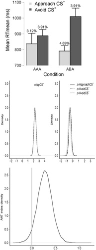
We next performed a Bayesian ANOVA, comparing a model that includes both main effects and the interaction (i.e., the full model) to a model that contains only the main effects (i.e., the restricted model). This comparison yielded a BF of 1.30. In Bayesian terms, this is “anecdotal evidence” for the full model that includes the interaction—in other words, the data are almost as likely under the restricted model as they are under the full model (Wetzels, Ravenzwaaij, & Wagenmakers, in press). In light of this result, we investigated the nature of the interaction of interest using separate Bayesian t-tests (Rouder, Speckman, Sun, Morey, & Iverson, 2009; Wetzels, Raaijmakers, Jakab, & Wagenmakers, 2009), comparing approach CS⁺ and avoid CS⁺ trials for each group separately. Results showed that although no effect of Response Assignment emerged for the AAA group (i.e., BF = .54), decisive evidence was obtained for the ABA group (i.e., BF = 501.82) indicating that participants were indeed faster to approach the CS⁺ than to avoid it. These results are in line with those obtained from the frequentist analysis.

General method—data-set 2

For consistency with our previous model fit, we did not separate the trials into approach and avoid CS⁺ as in the analysis of Van Gucht et al. (2008). Instead, different drift rates (v) were computed for each stimulus (CS⁺ vs. CS⁻) by response (Approach vs. Avoidance) combination. Note that we fitted the model to the data of each group (i.e., AAA and ABA) separately. For applying the model to each group, we used as a baseline the approach CS⁺ condition, in which the largest difference in RTs was observed compared to the other three conditions; all other drift rates were computed in reference to this baseline. Choosing any other drift rate as baseline yields identical results. Different T_er and a parameters were also computed for each group separately and the parameter z was again fixed to the middle of the two boundaries (i.e., a/2). Convergence and model fit were evaluated as they were for the analysis of the first data-set.³ We also computed the AAT index, similarly to how the AAT index was computed for the previous data-set, which was defined as the difference between the drift rate for congruent and incongruent trials, i.e., AAT_v = mean (Approach , Avoid )—mean (Approach , Avoid ).

Posterior distribution—data-set 2

All R-hat values were below 1.1, indicating successful convergence for all chains. Furthermore, all chains were visually inspected and they each resembled a “fat hairy caterpillar”.⁵ Last, after simulating data in a similar manner as was done for data-set 1, we plotted the real data against the simulated data for each group separately. Figures 9 and 10 of the online Supplementary material show that the model predictions match the real data quite well.

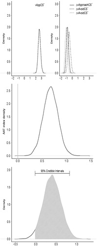
The middle panels of Figure 3 provide density plots of the posterior distributions for the different drift rates for the AAA group; the top panel of Figure 4 does the same for the ABA group.⁵ Note that in both cases, the drift rates in the left panel (i.e., Approach CS⁻, Avoid CS^– and Avoid CS⁺) are shown as differences with respect to the drift rate in the right panel (i.e., Approach CS⁺). Larger vs indicate faster information accumulation. The panel plot shows that the drift rate for the Approach CS⁺ trials is much higher than the other three drift rates, which largely overlap with each other. However, those differences seem to be more pronounced for the ABA group than for the AAA group. Regarding the AAT indices, the AAT index for the ABA group (see bottom panel of Figure 4) is positioned more to the right, indicating stronger approach tendencies, compared to the AAT index of the AAA group (see bottom panel of Figure 3). In order to quantify this difference, we obtained the posterior distribution for the differences in the AAT index between the ABA group and the AAA group, that is ΔAAT = AAT (ABA)—AAT (AAA). Then, we considered two order-estimated distinct hypotheses. The first hypothesis, H_>0, holds that the ΔAAT is positive, and the second hypothesis, H_<0, holds that the ΔAAT is negative. In order to quantify the support that the data provide for H_>0 versus H_<0, we can calculate a BF based on the posterior mean of ΔAAT that is greater than zero. The resulting BF is equal to 31.79 and the credible interval ranged from –.012 to 0.83 (see bottom panel of Figure 4). These results support the hypothesis that indeed, the ABA group accumulated information faster than the AAA group. As before, we note that these results are suggestive only, with a stricter test requiring a BF hypothesis test that includes a point null hypothesis. The development of such test is the topic of current investigation.

Figure 4. Top panel: Kernel density estimates of the posterior distributions for the drift rate parameters for the ABA group of the second data-set (Van Gucht et al., 2008), with results resembling those of the AAA group. The left panel shows the drift rate distribution for the Approach CS⁺ condition. The right panel shows the drift rate distributions for the Approach CS^–, Avoid CS^– and Avoid CS⁺ conditions, all relative to the Approach CS⁺ condition. Note that all depicted distributions refer to the group variables. From the results, it is apparent that (1) participants exhibited higher drift rate in the Approach CS⁺, compared to the other three conditions and (2) that the Approach CS^–, Avoid CS^– and Avoid CS⁺ conditions highly overlap with each other. Middle panel: The distribution of the group drift rate AAT index for the ABA group of data-set 2. The posterior mass is mostly positive, suggesting that, as expected, participants accumulated information faster on congruent compared to incongruent trials. In comparison to the AAT index of group AAA, this density is positioned more to the right, indicating stronger relative approach tendencies. Bottom panel: The posterior kernel estimate of the posterior distribution regarding the differences in AAT indices between the AAA and the ABA groups. The greyed area depicts the values above zero.

Discussion—data-set 2

The results of the second data-set show the expected patterns; participants exhibited higher speed of information accumulation in the approach CS⁺ condition than the other conditions. These differences were more pronounced in the ABA group, with larger differences between the different conditions, than in the AAA group. Nevertheless, the model was able to pick up differences between the various conditions for the AAA group, even when the main analyses did not seem to be able to detect any differences.

CONCLUDING COMMENTS

The goal of the present paper was to introduce a hierarchical Bayesian drift diffusion model decomposition of RT tasks. To illustrate the power of the approach, we have applied our model to the data of two studies that used the AAT, a commonly used task across experimental psychopathology, emotion research and social psychology, in which either avoidance (data-set 1) or approach (data-set 2) was the response of main interest. The descriptive results of data-set 1 indicate that participants accumulated information slower when they had to avoid the CS^– compared to the other three, largely similar, conditions. For data-set 2, results showed that participants accumulated information faster when they had to approach the CS⁺ than for any of the other conditions, which were largely similar as well. Furthermore, as was shown by the AAT drift rate indices, the between-conditions differences in data-set 2 were more pronounced in the ABA than in the AAA group.

The presented model has a number of advantages over data analysis techniques commonly used for RT tasks (see above). First, the entire RT distributions for correct as well as incorrect responses are included within a single inferential framework. This can lead to more complete performance predictions than when considering merely the central tendencies of RTs for speed and the proportion of correct responses for accuracy. Second, the model accounts for the positive relationship between speed and accuracy (Schouten & Bekker, 1967), a relationship that although always present in RT tasks is usually not considered in commonly applied analysis techniques.

Furthermore, our approach inherits the advantages from hierarchical modelling (Rouder & Lu, 2005; Shiffrin et al., 2008) and from Bayesian inference (Lee, 2011). First, hierarchical modelling features parameter estimation at the group level and at the level of the individual; the group-level parameters constrain the individual-level parameters, and the individual-level parameters inform the group-level parameters. Such reciprocal relations between the group and the individual parameters result in more complete and accurate predictions that can be applied both to particular individuals and to the population (Rouder & Lu, 2005). In addition, in Bayesian inference, parameter estimation is based both on the actual data and the parameter priors; consequently, meaningful results can be obtained even when only a limited number of trials per participant is available. These model features provide concrete advantages for psychologists, especially when dealing with clinical populations where the number of participants and the number of trials per individual are typically small and individual differences are at least as relevant as group-level performance.

Last, our model can shed light on the cognitive processes (e.g., response caution or speed of information accumulation) involved in RT decision-making tasks (Wagenmakers, 2009) and as such can give a detailed description of decision-making performance. This model's ability enables researchers to make more pluralistic and precise predictions as to which parameters will be affected by different experimental manipulations, enabling a deeper investigation of decision-making processes.

Here, we fit our model to two experimental data-sets in which either threatening (Experiment 1) or appetitive (Experiment 2) conditioned stimuli were used. Our model could just as well be applied to data-sets in which non-conditioned stimuli are considered (e.g., data on individuals with substance abuse disorder, Wiers et al., 2011). An advantage of using stimuli with pre-existing hedonic charge is that more trials per participant can be collected, something that should allow tests of models in which multiple parameters per condition are allowed to vary (Lewandowsky & Farrell, 2010).

Our measurement model was based on specific assumptions (i.e., any difference between conditions is captured by differences in drift rate rather than boundary separation, bias or non-decision time) that were based on specific characteristics of trial order and instructions provided in most AAT experiments. Modifications to the AAT procedure could warrant the use of alternative measurement models. For example, an experiment in which participants first see the CSs and then another irrelevant stimulus (e.g., an arrow), which indicates whether they have to approach or avoid each stimulus, may call for a model in which a-priori bias rather than information accumulation is allowed to differ per condition.

We have used the AAT as an example task for which our model can be used. Similar analyses could easily be applied to any other RT task (e.g. emotional Stroop task, dot-probe task and IAT). Of note, the application of Bayesian hierarchical models has increased our understanding of other types of emotion tasks as well (e.g., emotional flanker task; Pe et al., 2013; see also Vandekerckhove, Tuerlinckx, & Lee, 2011). We believe that the shift from commonly used techniques (e.g., ANOVAs) to cognitive modelling will allow a richer and more accurate inference on experimental data-sets (Lee, 2011; Wiecki, Poland & Frank, in press).

The computation of parameters in a hierarchical manner also enables a fuller investigation of individual differences, even when dealing with sparse data-sets. To date, individual differences in RT tasks are typically explored by either the computation of different RT indices for separate groups (e.g., Rinck & Becker, 2007; Wiers et al., 2009) or the use of correlations between some RT index and particular individual differences factors (Klein et al., 2011). Parameter extraction in terms of our model allows the testing of individual differences in terms of not only the RT index but also the psychological parameters involved in decision-making. In the study by Rinck and Becker (2007), for example, the researchers could have fit a standard regression model to the relation between the AAT index and spider fear, rather than separating the participants into groups with high and low spider phobia.

Despite its advantages, the presented analytic approach also has limitations. For example, our inference was based solely on the shape of the posterior distribution and did not feature a statistical null hypothesis test (e.g., see Gelman & Hill, 2007 for a similar approach in Bayesian regression modelling). We present our paper as a first detailed demonstration of the presented analytic technique, worthy of further research and elaboration. We also acknowledge that interested researchers face a start-up cost in getting to master the tools for applying diffusion models and performing hierarchical Bayesian parameter estimation. However, the wealth of available resources on cognitive modelling (e.g., Heathcote, Brown, & Wagenmakers, in press; and online Supplementary material) keeps such a cost to a minimum. Furthermore, we believe that the advantages of these novel analyses are well worth the effort.

In sum, we presented a Bayesian hierarchical psychological process model for analysing RT data that overcomes the pitfalls of previous analysis techniques. With the suggested model, researchers should be able to draw more robust and veridical conclusions from their data as the statistical results (1) take into account the uncertainty of each individual's estimate, (2) respect the speed–accumulation trade-off and (3) are based on estimates of the underlying decision-making processes. The practical applicability of the model was explored by accounting for findings from two real-life AAT data-sets. As more and more studies use RT tasks, we hope that the present approach will help researchers in the study of decision-making under conditions of speeded responding.

Supplementary material

Supplementary material is available via the ‘Supplementary’ tab on the article's online page (http://dx.doi.org/10.1080/02699931.2014.985635).

Notes

¹ As will be apparent later, the data-sets under consideration are sparse, with no more than 8 trials in each of four conditions, and error rates are low. In such situations—representative of real-world data-sets—adding more parameters to account for subtle effects is contraindicated.

² In the original experiment, participants were separated into two groups with half of the participants responding to a relevant stimulus feature (i.e., stimulus shape) and the other half to an irrelevant stimulus feature (i.e., the orientation of the surrounding frame). However, since no differences were found between the groups, we collapsed data across groups.

³ See online Supplementary material for more details on our modelling strategy and accompanying plots.

⁴ We chose the specific formula over alternatives ones (e.g., see AAT computation strategies B and C) as comparing congruent to incongruent trials is closer to how performance is evaluated in other stimulus compatibility tasks, such as the Simon task (see De Houwer et al., 2001 and the supplementary material of Krypotos et al., 2013 for more details).

⁵ See online Supplementary material for the relevant plots of all group parameters.

⁶ As we were mainly concerned with drift rates, we included the posterior distributions of the a and the Ter parameters in the online Supplementary material.

⁷ This result is suggestive only. A stricter test requires a Bayesian test using Bayes factors (Jeffreys, 1961; Lee & Wagenmakers, 2013; Rouder & Morey, 2012). The development of default Bayes factor hypothesis tests for hierarchical models is the topic of current statistical investigation.

REFERENCES

- Adams, R. B., Ambady, N., Macrae, C. N., & Kleck, R. E. (2006). Emotional expressions forecast approach-avoidance behavior. Motivation and Emotion, 30, 177–186. doi:10.1007/s11031-006-9020-2
- Batchelder, W. H. (1998). Multinomial processing tree models and psychological assessment. Psychological Assessment, 10, 331–344. doi:10.1037/1040-3590.10.4.331
- Bouton, M. E. (1993). Context, time, and memory retrieval in the interference paradigms of Pavlovian learning. Psychological Bulletin, 114(1), 80–99. doi:10.1037/0033-2909.114.1.80
- Bradley, M. M., & Lang, P. J. (2007). Emotion and motivation. Handbook of Psychophysiology, 3, 587–589.
- Chance, P. (1999). Thorndike's puzzle boxes and the origins of the experimental analysis of behavior. Journal of the Experimental Analysis of Behavior, 72, 433–440. doi:10.1901/jeab.1999.72-433
- Chen, M., & Bargh, J. A. (1999). Consequences of automatic evaluation: Immediate behavioral predispositions to approach or avoid the stimulus. Personality and Social Psychology Bulletin, 25, 215–224. doi:10.1177/0146167299025002007
- Cousijn, J., Goudriaan, A. E., & Wiers, R. W. (2011). Reaching out towards cannabis: Approach-bias in heavy cannabis users predicts changes in cannabis use. Addiction, 106, 1667–1674. doi:10.1111/j.1360-0443.2011.03475.x
- De Houwer, J., Crombez, G., Baeyens, F., & Hermans, D. (2001). On the generality of the affective Simon effect. Cognition & Emotion, 15, 189–206. doi:10.1080/02699930125883
- Dienes, Z. (2011). Bayesian versus orthodox statistics: Which side are you on? Perspectives on Psychological Science, 6, 274–290. doi:10.1177/1745691611406920
- Dutilh, G., Krypotos, A.-M., & Wagenmakers, E.-J. (2011). Task-related versus stimulus-specific practice: A diffusion model account. Experimental Psychology, 58, 434–442. doi:10.1027/1618-3169/a000111
- Dyjas, O., Grasman, R. P., Wetzels, R., van der Maas, H. L., & Wagenmakers, E.-J. (2012). What's in a name: A Bayesian hierarchical analysis of the name-letter effect. Frontiers in Psychology, 3, 334.
- Eberl, C., Wiers, R. W., Pawelczack, S., Rinck, M., Becker, E. S., & Lindenmeyer, J. (2013). Implementation of approach bias re-training in alcoholism: How many sessions are needed? Alcoholism: Clinical and Experimental Research, 38, 587–594. doi:10.1111/acer.12281
- Edwards, W., Lindman, H., & Savage, L. J. (1963). Bayesian statistical inference for psychological research. Psychological Review, 70, 193–242. doi:10.1037/h0044139
- Effting, M., & Kindt, M. (2007). Contextual control of human fear associations in a renewal paradigm. Behaviour Research and Therapy, 45, 2002–2018. doi:10.1016/j.brat.2007.02.011
- Efron, B., & Morris, C. (1977). Stein's paradox in statistics. Scientific American, 236(5), 119–127. doi:10.1038/scientificamerican0577-119
- Frijda, N. H. (1988). The laws of emotion. American Psychologist, 43, 349–358. doi:10.1037/0003-066X.43.5.349
- Gelman, A., & Hill, J. (2007). Data analysis using regression and multilevel/hierarchical models. Cambridge: Cambridge University Press.
- Greenwald, A. G., McGhee, D. E., Schwartz, J. L. K. (1998). Measuring individual differences in implicit cognition: The implicit association test. Journal of Personality and Social Psychology, 74, 1464–1480. doi:10.1037/0022-3514.74.6.1464
- Hays, W. L. (1973). Statistics for the social sciences (Vol. 410). New York, NY: Holt, Rinehart and Winston.
- Heathcote, A., Brown, S., & Mewhort, D. (2000). The power law repealed: The case for an exponential law of practice. Psychonomic Bulletin & Review, 7, 185–207. doi:10.3758/BF03212979
- Heathcote, A., Brown, S. D., & Wagenmakers, E.-J. (in press). An introduction to good practices in cognitive modeling. In B. U. Forstmann & E.-J. Wagenmakers (Eds.), An introduction to model-based cognitive neuroscience. New York, NY: Springer.
- Heathcote, A., Popiel, S. J., & Mewhort, D. J. (1991). Analysis of response time distributions: An example using the Stroop task. Psychological Bulletin, 109, 340–347. doi:10.1037/0033-2909.109.2.340
- Heuer, K., Rinck, M., & Becker, E. S. (2007). Avoidance of emotional facial expressions in social anxiety: The Approach-Avoidance Task. Behaviour Research and Therapy, 45, 2990–3001. doi:10.1016/j.brat.2007.08.010
- Ho, T. C., Yang, G., Wu, J., Cassey, P., Brown, S. D., Hoang, N., … Yang, T. T. (2014). Functional connectivity of negative emotional processing in adolescent depression. Journal of Affective Disorders, 155, 65–74. doi:10.1016/j.jad.2013.10.025
- Jeffreys, H. (1961). Theory of probability (3rd ed.). Oxford: Oxford University Press.
- Klein, A. M., Becker, E. S., & Rinck, M. (2011). Approach and avoidance tendencies in spider fearful children: The Approach-Avoidance Task. Journal of Child and Family Studies, 20, 224–231. doi:10.1007/s10826-010-9402-7
- Krieglmeyer, R., & Deutsch, R. (2010). Comparing measures of approach–avoidance behaviour: The manikin task vs. two versions of the joystick task. Cognition and Emotion, 24, 810–828. doi:10.1080/02699930903047298
- Kristjansson, S. D., Kircher, J. C., & Webb, A. K. (2007). Multilevel models for repeated measures research designs in psychophysiology: An introduction to growth curve modeling. Psychophysiology, 44, 728–736. doi:10.1111/j.1469-8986.2007.00544.x
- Krypotos, A.-M., Effting, M., Arnaudova, I., Kindt, M., & Beckers, T. (2014). Avoided by association: Acquisition, extinction, and renewal of avoidance tendencies towards conditioned fear stimuli. Clinical Psychological Science, 2, 336–343. doi:10.1177/2167702613503139
- Lang, P. J. (1985). The cognitive psychophysiology of emotion: Fear and anxiety. In H. Tuma & J. Maser (Eds.), Anxiety and the anxiety disorders (pp. 131–170). Hillsdale, NJ: Erlbaum.
- Lang, P. J., & Bradley, M. M. (2008). Appetitive and defensive motivation is the substrate of emotion. In A. J. Elliot (Ed.), Handbook of approach and avoidance motivation (pp. 51–65). New York, NY: Psychology Press.
- Lee, M. D. (2011). How cognitive modeling can benefit from hierarchical Bayesian models. Journal of Mathematical Psychology, 55(1), 1–7. doi:10.1016/jjmp.2010.08.013
- Lee, M. D., & Wagenmakers, E.-J. (2013). Bayesian modeling for cognitive science: A practical course. Cambridge: Cambridge University Press.
- Leite, F. P., & Ratcliff, R. (2011). What cognitive processes drive response biases? A diffusion model analysis. Judgment and Decision Making, 6, 651–687.
- Lewandowsky, S., & Farrell, S. (2010). Computational modeling in cognition: Principles and practice. Thousand Oaks, CA: Sage.
- Luce, R. (1986). Response times: Their role in inferring elementary mental organization. Oxford, New York: Oxford University Press.
- Lynch, S. M. (2007). Introduction to applied Bayesian statistics and estimation for social scientists. New York, NY: Springer.
- MacLeod, C., Mathews, A., Tata, P. (1986). Attentional bias in emotional disorders. Journal of Abnormal Psychology, 95(1), 15–20. doi:10.1037/0021-843X.95.1.15
- Matzke, D., & Wagenmakers, E.-J. (2009). Psychological interpretation of the ex-Gaussian and shifted Wald parameters: A diffusion model analysis. Psychonomic Bulletin & Review, 16, 798–817. doi:10.3758/PBR.16.5.798
- McAuley, T., Yap, M., Christ, S. E., & White, D. A. (2006). Revisiting inhibitory control across the life span: Insights from the ex-Gaussian distribution. Developmental Neuropsychology, 29, 447–458. doi:10.1207/s15326942dn2903_4
- Mead, R. (1990). The design of experiments: Statistical principles for practical applications. Cambridge: Cambridge University Press.
- Miller, J. (1988). A warning about median reaction time. Journal of Experimental Psychology: Human Perception and Performance, 14, 539–543. doi:10.1037/0096-1523.14.3.539
- Morey, R. D., Pratte, M. S., & Rouder, J. N. (2008). Problematic effects of aggregation in zROC analysis and a hierarchical modeling solution. Journal of Mathematical Psychology, 52, 376–388. doi:10.1016/j.jmp.2008.02.001
- Mulder, M. J., Wagenmakers, E.-J., Ratcliff, R., Boekel, W., & Forstmann, B. U. (2012). Bias in the brain: A diffusion model analysis of prior probability and potential payoff. The Journal of Neuroscience, 32, 2335–2343. doi:10.1523/JNEUROSCI.4156-11.2012
- Neumann, R., Hülsenbeck, K., & Seibt, B. (2004). Attitudes towards people with AIDS and avoidance behavior: Automatic and reflective bases of behavior. Journal of Experimental Social Psychology, 40, 543–550. doi:10.1016/j.jesp.2003.10.006
- Nilsson, H., Rieskamp, J., & Wagenmakers, E. (2011). Hierarchical Bayesian parameter estimation for cumulative prospect theory. Journal of Mathematical Psychology, 55(1), 84–93. doi:10.1016/j.jmp.2010.08.006
- Pachella, R. G. (1974). The interpretation of reaction time in information-processing research. In B. H. Kantowitz (Ed.), Human information processing: Tutorials in performance and cognition (pp. 41–82). Hillsdale, NJ: Lawrence Erlbaum Associates.
- Pe, M. L., Vandekerckhove, J., & Kuppens, P. (2013). A diffusion model account of the relationship between the emotional flanker task and rumination and depression. Emotion, 13, 739–747. doi:10.1037/a0031628
- Ratcliff, R. (1978). A theory of memory retrieval. Psychological Review, 85, 59–108. doi:10.1037/0033-295X.85.2.59
- Ratcliff, R. (1979). Group reaction time distributions and an analysis of distribution statistics. Psychological Bulletin, 86, 446–461. doi:10.1037/0033-2909.86.3.446
- Ratcliff, R. (1993). Methods for dealing with reaction time outliers. Psychological Bulletin, 114, 510–532. doi:10.1037/0033-2909.114.3.510
- Ratcliff, R. (2002). A diffusion model account of response time and accuracy in a brightness discrimination task: Fitting real data and failing to fit fake but plausible data. Psychonomic Bulletin & Review, 9, 278–291. doi:10.3758/BF03196283
- Ratcliff, R., & McKoon, G. (2008). The diffusion decision model: Theory and data for two–choice decision tasks. Neural Computation, 20, 873–922. doi:10.1523/JNEUROSCI.3733-05.2006
- Ratcliff, R., & Tuerlinckx, F. (2002). Estimating parameters of the diffusion model: Approaches to dealing with contaminant reaction times and parameter variability. Psychonomic Bulletin & Review, 9, 438–481. doi:10.3758/BF03196302
- Rinck, M., & Becker, E. S. (2007). Approach and avoidance in fear of spiders. Journal of Behavior Therapy and Experimental Psychiatry, 38(2), 105–120. doi:10.1016/j.jbtep.2006.10.001
- Rouder, J. N., & Lu, J. (2005). An introduction to Bayesian hierarchical models with an application in the theory of signal detection. Psychonomic Bulletin & Review, 12, 573–604. doi:10.3758/BF03196750
- Rouder, J. N., & Morey, R. D. (2012). Default Bayes factors for model selection in regression. Multivariate Behavioral Research, 47, 877–903. doi:10.1080/00273171.2012.734737
- Rouder, J. N., Morey, R. D., Speckman, P. L., & Province, J. M. (2012). Default Bayes factors for ANOVA designs. Journal of Mathematical Psychology, 56, 356–374. doi:10.1016/j.jmp.2012.08.001
- Rouder, J. N., Speckman, P. L., Sun, D., Morey, R. D., & Iverson, G. (2009). Bayesian t tests for accepting and rejecting the null hypothesis. Psychonomic Bulletin & Review, 16, 225–237. doi:10.3758/PBR.16.2.225
- Rutherford, H. J. V., & Lindell, A. K. (2011). Thriving and surviving: Approach and avoidance motivation and lateralization. Emotion Review, 3, 333–343. doi:10.1177/1754073911402392
- Salemink, E., van den Hout, M. A., & Kindt, M. (2007). Selective attention and threat: Quick orienting versus slow disengagement and two versions of the dot probe task. Behaviour Research and Therapy, 45, 607–615. doi:10.1016/j.brat.2006.04.004
- Schouten, J. F., & Bekker, J. A. M. (1967). Reaction time and accuracy. Acta Psychologica, 27, 143–153. doi:10.1016/0001-6918(67)90054-6
- Sellke, T., Bayarri, M., & Berger, J. O. (2001). Calibration of ρ values for testing precise null hypotheses. The American Statistician, 55(1), 62–71. doi:10.1198/000313001300339950
- Shiffrin, R., Lee, M., Kim, W., & Wagenmakers, E.-J. (2008). A survey of model evaluation approaches with a tutorial on hierarchical Bayesian methods. Cognitive Science, 32, 1248–1284. doi:10.1080/03640210802414826
- Smith, P. L., & Ratcliff, R. (in press). A tutorial on the diffusion model of decision making. In B. U. Forstmann & E.-J. Wagenmakers (Eds.), An introduction to model–based cognitive neuroscience. New York, NY: Springer.
- Spruyt, A., De Houwer, J., Tibboel, H., Verschuere, B., Crombez, G., Verbanck, P., … Noël, X. (2013). On the predictive validity of automatically activated approach/avoidance tendencies in abstaining alcohol-dependent patients. Drug and Alcohol Dependence, 127(1–3), 81–86. doi:10.1016/j.drugalcdep.2012.06.019
- Strauss, G. P., Frank, M. J., Waltz, J. A., Kasanova, Z., Herbener, E. S., & Gold, J. M. (2011). Deficits in positive reinforcement learning and uncertainty-driven exploration are associated with distinct aspects of negative symptoms in schizophrenia. Biological Psychiatry, 69, 424–431. doi:10.1016/j.biopsych.2010.10.015
- Stroop, J. R. (1935). Studies of interference in serial verbal reactions. Journal of Experimental Psychology, 18, 643–662. doi:10.1037/h0054651
- Vandekerckhove, J., Tuerlinckx, F., & Lee, M. D. (2011). Hierarchical diffusion models for two-choice response times. Psychological Methods, 16(1), 44–62. doi:10.1037/a0021765
- Van Gucht, D., Vansteenwegen, D., Van den Bergh, O., & Beckers, T. (2008). Conditioned craving cues elicit an automatic approach tendency. Behaviour Research and Therapy, 46, 1160–1169. doi:10.1016/j.brat.2008.05.010
- van Ravenzwaaij, D., Dutilh, G., & Wagenmakers, E.-J. (2012). A diffusion model decomposition of the effects of alcohol on perceptual decision making. Psychopharmacology, 219, 1017–1025. doi:10.1007/s00213-011-2435-9
- Vansteenwegen, D., Hermans, D., Vervliet, B., Francken, G., Beckers, T., Baeyens, F., Eelen, P. (2005). Return of fear in a human differential conditioning paradigm caused by a return to the original acquistion context. Behaviour Research and Therapy, 43, 323–336. doi:10.1016/j.brat.2004.01.001
- Voncken, M., Rinck, M., Deckers, A., & Lange, W.-G. (2011). Anticipation of social interaction changes implicit approach-avoidance behavior of socially anxious individuals. Cognitive Therapy and Research, 36, 1–10.
- Vrijsen, J. N., van Oostrom, I., Speckens, A., Becker, E. S., & Rinck, M. (2013). Approach and avoidance of emotional faces in happy and sad mood. Cognitive Therapy and Research, 37(1), 1–6. doi:10.1007/s10608-012-9436-9
- Wagenmakers, E.-J. (2007). A practical solution to the pervasive problems of p values. Psychonomic Bulletin & Review, 14, 779–804. doi:10.3758/BF03194105
- Wagenmakers, E.-J. (2009). Methodological and empirical developments for the Ratcliff diffusion model of response times and accuracy. European Journal of Cognitive Psychology, 21, 641–671. doi:10.1080/09541440802205067
- Wagenmakers, E.-J., & Brown, S. (2007). On the linear relation between the mean and the standard deviation of a response time distribution. Psychological Review, 114, 830–841. doi:10.1037/0033-295X.114.3.830
- Wagenmakers, E.-J., van der Maas, H. L. J., & Grasman, R. P. P. P. (2007). An EZ–diffusion model for response time and accuracy. Psychonomic Bulletin & Review, 14(1), 3–22. doi:10.3758/BF03194023
- Wetzels, R., Grasman, R. P. P. P., & Wagenmakers, E.-J. (2012). A default Bayesian hypothesis test for ANOVA designs. The American Statistician, 66(2), 104–111. doi:10.1080/00031305.2012.695956
- Wetzels, R., Raaijmakers, J. G. W., Jakab, E., & Wagenmakers, E.-J. (2009). How to quantify support for and against the null hypothesis: A flexible WinBUGS implementation of a default Bayesian t–test. Psychonomic Bulletin & Review, 16, 752–760. doi:10.3758/PBR.16.4.752
- Wetzels, R., van Ravenzwaaij, D., & Wagenmakers, E.-J. (in press). Bayesian analysis. In R. Cautin & S. Lilienfeld (Eds.), The Encyclopedia of Clinical Psychology. Wiley-Blackwell.
- White, C. N., Ratcliff, R., Vasey, M. W., & McKoon, G. (2010a). Anxiety enhances threat processing without competition among multiple inputs: A diffusion model analysis. Emotion, 10, 662–677. doi:10.1037/a0019474
- White, C. N., Ratcliff, R., Vasey, M. W., & McKoon, G. (2010b). Using diffusion models to understand clinical disorders. Journal of Mathematical Psychology, 54(1), 39–52. doi:10.1016/j.jmp.2010.01.004
- Wiecki, T., Poland, J. S., & Frank, M. J. (in press). Model-based cognitive neuroscience approaches to computational psychiatry: Clustering and classification. Clinical Psychological Science.
- Wiecki, T. V., Sofer, I., & Frank, M. J. (2013). HDDM: Hierarchical Bayesian estimation of the drift–diffusion model in Python. Frontiers in Neuroinformatics, 7, 14. doi:10.3389/fninf.2013.00014
- Wiers, R. W., Eberl, C., Rinck, M., Becker, E., & Lindenmeyer, J. (2011). Retraining automatic action tendencies changes alcoholic patients approach bias for alcohol and improves treatment outcome. Psychological Science, 22, 490–497. doi:10.1177/0956797611400615
- Wiers, R. W., Rinck, M., Dictus, M., & Van den Wildenberg, E. (2009). Relatively strong automatic appetitive action-tendencies in male carriers of the OPRM1 G-allele. Genes, Brain and Behavior, 8(1), 101–106. doi:10.1111/j.1601-183X.2008.00454.x
- Wiers, R. W., Rinck, M., Kordts, R., Houben, K., & Strack, F. (2010). Retraining automatic action-tendencies to approach alcohol in hazardous drinkers. Addiction, 105, 279–287. doi:10.1111/j.1360-0443.2009.02775.x
- Williams, J. M., Mathews, A., MacLeod, C. (1996). The emotional Stroop task and psychopathology. Psychological Bulletin, 120(1), 3–24. doi:10.1037/0033-2909.120.1.3