Emission measurements with gravimetric impactors and electrical devices: An aerosol instrument comparison

Abstract

Particulate matter in the atmosphere is known to affect Earth’s climate and to be harmful to human health. Accurately measuring particles from emission sources is important, as the results are used to inform policies and climate models. This study compares the results of two ELPI + devices, two PM10 cascade impactors and an eFilter, in combustion emission measurements. The comparison of the instruments in a realistic setting shows what types of challenges arise from measuring an emission aerosol with unknown particle morphologies and densities, different particle concentrations and high temperature. Our results show that the PM10 cascade impactors have very good intercorrelation when the collected mass is greater than 150 µg, but below that, the uncertainty of the results increases with decreasing mass. The raw signals of two ELPI + devices were nearly identical in most samples, as well as the particle number concentrations and size distributions calculated from raw signals; however, transforming the current distributions into mass distributions showed variation in the mass concentration of particles larger than 1 µm. The real-time time signal measured by eFilter was similar to the total current measured by ELPI+. The eFilter and PM10 cascade impactors showed similar particle mass concentrations, whereas ELPI + showed clearly higher ones in most cases. We concluded that the difference is at least partially due to volatile components being measured by ELPI+, but not by the mass collection measurements.

Copyright © 2019 American Association for Aerosol Research

1. Introduction

Anthropogenic aerosols are of great concern, as it is well-established that they are harmful to human health (e.g. Lelieveld et al. 2015) and have climate effects (e.g. Andreae, Jones, and Cox 2005; Lee, Reddington, and Carslaw 2016).Combustion emissions are a major source of atmospheric particle pollution. To understand their full effect on health and climate, researchers create dispersion and climate models to predict effects. These models require accurate measurements directly from the emission source as input. Otherwise, inaccuracies in measurements are passed onto the models, and the inaccurate models are used to inform decision making and environmental policies. One established way to gain information on the instrument performance is to compare results from instruments in concurrent measurements.

In atmospheric aerosol measurements, instrument comparisons are commonplace. For example, Hitzenberger et al. (2004) compared more than 50 mass measurement instruments in their atmospheric aerosol study, including Electrical Low Pressure Impactor (ELPI) and several cascade impactors. In combustion emission measurements, results for each studied characteristic (particle number concentration, mass concentration, size distribution, etc.) are often reported based on the measurement data from a single instrument. Instruments are of course calibrated before use, but laboratory calibration is conducted with known particle material, concentration and size distribution, under controlled environmental conditions. Considering the harsh conditions of emission measurements—high temperatures, varying pressure, high particle concentrations—and the rapidly changing source, it would be surprising not to encounter any discrepancies between instruments. In addition to the conditions within the tubing, the surroundings create challenges as well: vibrations from moving components, high or low temperatures and tight spaces. Small differences in operation methods by different users may also have noticeable effects on the results.

Instrument comparisons between different instances of combustion emission measurements are difficult, as sampling methods are also known to affect results (Burtscher 2005; Lipsky and Robinson 2006; Rönkkö et al. 2006). Despite the general lack of comparison studies, some instrument pairs have been studied: ELPI and Scanning Mobility Particle Sizer (SMPS) in particle size distribution measurements (Amaral et al. 2015; Maricq, Podsiadlik, and Chase 2000; Marjamäki et al. 2000), SMPS and Engine Exhaust Particle Sizer (EEPS) in particle size distribution measurements (Xue et al. 2015) and ELPI and gravimetric impactor particle mass concentration in the submicron size-range (Maricq, Xu, and Chase 2006). As far as we could tell, only one previous study compared identical instruments (condensation particle counters) in the same combustion emission measurement (Petzold et al. 2011).

In addition to accuracy, other instrument properties to consider when choosing instruments for a measurement setup are price, time resolution, size, measurement output, and how much maintenance is required. Aerosol measurement techniques can be divided into two main groups: offline and online, with the former generally being the more inexpensive method upfront (Dhaniyala et al. 2011). Collecting particles with an impactor or filter are types of offline measurements. Although the instruments are inexpensive, the collected substrates require handling, consuming work hours. Online instruments are generally more expensive, but offer numerous benefits: high time-resolution, instantaneous results and fewer work hours. When it comes to measurement output, mass concentration is commonly used, as particle air quality standards are defined by mass concentration (“Air Quality Standards” 2017). Particle number is also commonly measured, as small particles are not well represented by mass, and particle number emissions are limited for vehicles. When possible, it is better to measure both in order to get a full picture of the emissions.

In this study, we present a comparison of five aerosol measurement instruments: two PM10 gravimetric cascade impactors (Dekati Ltd., Kangasala, Finland), two ELPI+’s (Dekati Ltd.) and one eFilter (Dekati Ltd.). The instruments were used to measure flue gas from oil shale and wood combustion. Data from each instrument was then used to calculate the mass concentration of particles in the flue gases. Additionally, the electrical currents measured by eFilter and ELPI + were compared. The two measured emission types, oil shale and wood, contained highly different concentrations of particles, giving a good range of data. The purpose of our study is to report on the correlation of results from essentially identical instruments operated by different research groups, to discover limitations of the selected instruments by comparing results, and to discuss the reliable utilization of these instruments for emission measurements. We also hope to encourage a culture of instrument comparison studies in combustion emission measurements.

2. Materials and methods

2.1. Instrument descriptions

The three instrument types used in this study are summarized in Table 1. ELPI + is an online device, whereas the PM10 cascade impactor is offline. The eFilter is a hybrid, measuring electrical current while simultaneously collecting particulate mass onto a filter, which needs to be weighed. In addition to the studied instruments, an SMPS was in use during the measurements, but the data is only included in the supplementary material, as it was not part of the initial study design.

Table 1. Information on the three instrument types used in this study.

Instruments used in this study	Flow rate (L/min)	Particle sizes measured	Data outputs	Other information
ELPI+ (x2)	10	6 nm–10 µm	Stage-specific electrical current	Current size distribution may be processed into number and mass distributions. Cutoff sizes for impactor stages (µm): [10 5.3 3.6 2.5 1.6 0.94 0.60 0.38 0.25 0.15 0.094 0.054 0.030 0.016 0.006]
PM10 gravimetric cascade impactor (x2)	10	0 nm–10 µm	Sampling time averaged mass concentration of three particle size ranges: 0–1 µm, 1–2.5 µm, 2.5–10 µm	There are three cut points (impactors) at particle diameters 10 µm, 2.5 µm, and 1 µm. The remaining particles are collected with a filter.
eFilter (x1)	20 (mass collection) and 0.5 (electrical measurement)	0 nm <	Sampling time averaged total mass concentration and related real-time electrical current	Combining the data outputs gives an estimation of the time-resolved mass concentration.

PM10 gravimetric cascade impactors (Dekati Ltd.) are used to measure the mass concentration of particles smaller than 10 µm in aerodynamic diameter. Incoming particles are deposited on collection plates by impaction. The PM10 impactors in this study also have an impactor cutoff at 2.5 µm, and another at 1 µm. A filter collects any remaining particles (less than 1 µm in aerodynamic diameter). Thus, they can also be used to determine PM_2.5 and PM₁. These impactors are commonly used in atmospheric measurements as well as measurements from an emission source. They fulfill the requirements for ISO23210, which sets the standard for particle mass concentration measurements from stationary emission sources.

ELPI+, as well as its predecessor ELPI (Dekati Ltd) (Keskinen, Pietarinen, and Lehtimäki 1992), is widely used for both atmospheric and emission measurements (Brachert et al. 2014; Duan et al. 2012; Liu et al. 2011; Maricq, Xu, and Chase 2006; Pirjola et al. 2017). The ELPI + includes an impactor with 14 stages, each connected to an electrometer. The particles entering the device are electrically charged and then classified by aerodynamic diameter in the cascade impactor. The charged and impacted particles impart an electrical current, which is then recorded. The current from each stage can be converted into a particle number concentration, and together the fourteen stages give the number size distribution. The particle number distribution can also be converted to other distributions, such as particle surface area, volume and mass. The ELPI+ (and ELPI) time resolution is 1 s, making it useful for measuring transient particle size distributions. The particle size range measureable by ELPI + is approximately 6 nm to 10 µm. Calibration coefficients and stage-specific cutoff sizes for the ELPI + are reported in Järvinen et al. (2014).

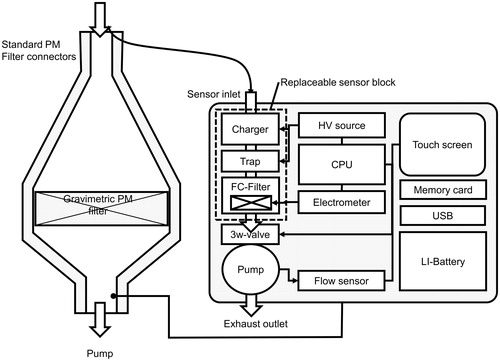
The eFilter (Dekati Ltd.), marketed since 2016, combines electrical measurement and gravimetric mass collection of particles. The benefit of this novel two-pronged approach is that it allows the user to see the changes in the particle concentration during the gravimetric particle collection. The instrument components and operation principle can be seen in Figure 1. The instrument has a large primary flowrate of 20–100 lpm through a 47 mm collection filter and a secondary flowrate of 0.5 lpm for the electrical measurement (through the replaceable sensor block). The secondary flow is generated with an internal pump, and it does not affect the gravimetric collection. The electrical portion of the instrument first charges incoming particles with a corona charger and then collects the particles onto a fiberglass filter inside a Faraday-cup connected to an electrometer. Electrical measurement is automatically switched on when the instrument detects the primary flow. This is useful, as the filter collection time then corresponds to the electrical measurement. The data output of the instrument is the current measured from the diffusion charged particles. If necessary, the electrical portion may also be used separately, i.e., independently of the filter collection of particles. In this study, quartz filters were used for the gravimetric collection. They were weighed as described in Section 2.2. The filter collection could also be used to perform chemical analysis of the sample.

Figure 1. Graphical representation of the eFilter operation principle, image provided by Dekati^®.

2.2. Measurements

Table 2 displays the different measurement cases. The first six measurements were for oil shale combustion, and final twelve for wood combustion, with three different subcases: wood, wood and waste, and wood and a concentrated soot remover (Hansa™, UAB Triju artele, Kaišiadorys, Lithuania). For the wood combustion, one measurement was taken during each ignition phase and three during the normal burning phase. Oil shale tests were conducted at a 60 kWth Circulating Fluidized Bed (CFB) combustion test facility in Tallinn University of Technology, described in detail in Konist et al. (2018). In this facility, the fluidized bed is produced from mineral matter of the oil shale; the amount of mineral matter can be 43–53% of the original mass of the fuel (Konist et al. 2016). The CFB facility was operated with its normal circulation and temperature profile. Wood combustion tests were carried out in the Estonian Environmental Research Centre (EERC) stove laboratory, using a 3500 kg brick made masonry heater, which is built according to the standard “EN 15544 One off Kachelgrundöfen/Putzgrundöfen (tiled/mortared stoves) – Dimensioning”. Logwood from three species, spruce (Picea abies), alder (Alnus incana) and pine (Pinus silvestris), was used. In each case, the wood was cut into pieces of 0.4–0.5 m length and split into halves or quarters. The wood was stored in a conventional way in an outdoor woodshed and was brought to stove laboratory at least 1 day prior to combustion experiment. Fuel was ignited from the top, in order to ensure good startup for the wood ignition. The wood moisture content ranged between 14% and 18% on wet basis. Each log batch was weighed, the heating value was measured and the relative humidity of each log was measured separately.

Table 2. Information on the measured combustion cases, the sampling times for PM10 cascade impactors and the dilution ratios for ELPI + and eFilter. The cascade impactors measured the flue gas undiluted.

	Fuel	Details	Sampling time (min)	Dilution ratio (ELPI + and eFilter)
1	Oil-shale		75	84
2	Oil-shale		94	9.6
3	Oil-shale		90	9.6
4	Oil-shale		70	9.6
5	Oil-shale		96	10
6	Oil-shale		30	10
7	Wood	Ignition	20	80
8	Wood	Burning	5	80
9	Wood	Burning	10	80
10	Wood	Burning	10	86
11	Wood + waste	Ignition	10	86
12	Wood + waste	Burning	10	86
13	Wood + waste	Burning	10	86
14	Wood + waste	Burning	10	86
15	Wood + soot remover	Ignition	7	177
16	Wood + soot remover	Burning	10	177
17	Wood + soot remover	Burning	10	177
18	Wood + soot remover	Burning	10	177

One research group operated one ELPI + and one PM10 cascade impactor, while the other two identical devices were operated by the other group. This article will refer to these research groups as group A and group B. The measurement setups are shown in Figure 2a (cascade impactors) and Figure 2b (ELPI + and eFilter). The two PM10 cascade impactors sampled for the exact same time periods in order to allow comparison. The other instruments sampled for longer periods. For the purposes of this article, only the data for the times matching the cascade impactor samples was compared.

Figure 2. Measurement setups for (a) the PM10 cascade impactors and (b) ELPI + and eFilter. The second ejector diluter, drawn in dashed lines, was used in the first oil shale measurement and all of the wood measurements. The PM10 cascade impactors, along with the cyclones were heated to approximately 90 °C and 135 °C in the oil shale and wood cases, respectively.

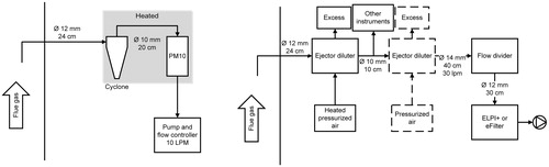
The PM10 cascade impactors each had their own sampling tubes of the same length, diameter, and bends, as well as identical cyclones to remove large particles. The inlets were oriented parallel to the surrounding flow. The only notable difference between the oil shale and wood combustion experiments was in the heating of the cyclone and PM10 cascade impactor, as it was about 80–100 °C in the oil shale cases and 120–150 °C in the wood cases. The nominal volumetric flowrate through the PM10 impactor needs to be 10 lpm for the cutoffs of 10 µm, 2.5 µm, and 1.0 µm. For PM10 A the flow was controlled with a mass flow controller (Alicat, Alicat Scientific, USA ), set to 10 SLPM. The PM10 B flow rate was controlled using Aquaria CF-20 Alfa Basic (AQUARIA Srl, Lacchiarella (MI), Italy) pump, where flow rate is measured with the high precision flow-meters and the flow rate was set to 10 SLPM. Because the cascade impactors were heated, the true cutoff particle diameters varied slightly, at most 6% from the given values, calculated according to Hering (1995). The difference was not taken into account in the results. In preparation for sampling, the PM10 cascade impactors and cyclone were allowed to heat up for about 20 min before each run. If they were still warm from the previous sampling run, this time was shorter. The cascade impactor plates were covered with greased foils, which were changed for each sample, and the used foils were stored for weighing. The PM10 cascade impactor filter, which collects the smallest particles, was similarly changed and stored for weighing between each measurement. The PM10 impactors were clean before beginning the experiments and were cleaned in an ultrasonic bath after the first sampling from wood combustion, as they were visibly soot-covered.

Both ELPI + instruments measured after dilution of the flue gas, at the same distance from the source. The flue gas was diluted with an ejector diluter (Dekati Ltd.), in which heated (70 °C) and pressurized air was used for dilution. The setups for wood and oil shale experiments were almost identical, but in the wood combustion case, an additional ejector diluter was used. The flow rate in ELPI + is 10 lpm, and it is controlled by a critical orifice within the instrument. Before measuring, the ELPI + collection plates were covered with greased foils. The foils were changed daily to avoid measurement error due to particles bouncing. ELPI + devices were switched on about an hour in advance, to allow their electrometers to settle before actual measurement. Instruments’ outlet pressures were checked to be 40 mbar and adjusted accordingly. The instruments were zeroed by sampling room air through a HEPA-filter, and administering the zeroing routine from the software menu. After zeroing, the HEPA-filter was left in place for 5–10 min to check that the zero levels did not change. The corona needle of the ELPI + A was cleaned twice during the measurement campaign.

The eFilter measured from the same location as the ELPI + instruments and used the same dilution system. The flowrate to the gravimetric filter was 20 lpm—the total sampled volume was measured using a pump with integrated flow measurement. The flowrate through the electrical measurement portion of the eFilter was 0.5 lpm, taken from the main flow, as seen in Figure 1. The eFilter was switched on at least 30 min before the measurement in order to stabilize the electronics temperatures. Sampling was started and stopped manually by switching on and off the gravimetric sample pump. This started also the electrical measurement and data logging. Electrical data was saved to a memory card for further data processing. After measurement, the sample filter was removed for gravimetric analysis. The weighing procedure was the same as for the PM10 cascade impactors.

The ELPI + and PM10 impactor foils were greased with Dekati^® Collection Substrate Spray to improve particle attachment. The PM10 filters and impactor foils were weighed before and after sampling. The filters were heated to 200 °C for 2 h, before sampling, and to 160 °C for 1 h after sampling, to remove moisture. After sampling and before weighing, the foils were allowed to cool inside a desiccator for at least 1 h and the filters for 2 h, as temperature can affect the weighing. The weighing room conditions were controlled and set to 50% humidity and a temperature of 22 °C. The foils and filters were weighed with a Kern 770 balance (10 µg precision).

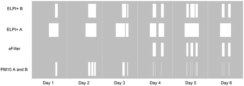
A blockage occurred in the second ejector diluter during sample 11, which affected the ELPI + and eFilter results. For the eFilter, this means that also the particle mass concentration for sample 12 must be excluded, as it was collected with the same filter as sample 11. Figure 3 shows the times when each instrument was sampling the aerosol.

Figure 3. The white boxes show the times when the specified instrument (y-axis) has been actively measuring. For eFilter and PM10 A and B, this means the duration of mass collection. The black rectangle shows the times when the ejector diluter was blocked, and affected eFilter and ELPI + measurements.

2.3. Data processing

2.3.1. pm10

The PM10 size fractioned results were obtained from the difference in collection foil and filter masses before and after sampling. Each particle mass concentration was calculated by dividing the collected particulate mass by the volume of aerosol sampled. The sampled volume was calculated by multiplying the sample flow rate by the sampling time.

2.3.2. elpi+

The ELPI + results were obtained using the datasheet provided by Dekati Ltd., and entering the required beginning and ending times for each measurement. We used 1 g/cm³ as the particle density setting and 1 as the dilution ratio (corrected later to reflect the true dilution ratio). the data sheet first applies a simple non-iterative calculation algorithm (Moisio 1999) to correct the current values for the secondary collection of sub-cut diameter particles (Virtanen et al. 2001). Then the number concentration is calculated from (1) $$N=\frac{I}{\mathit{eQ}\text{Pn}}\left[\frac{1}{c{m}^3}\right]$$(1) where is the current measured from an impactor stage, is the elementary charge (1.602e − 19 C), is the flowrate. The term is a particle diameter dependent product of particle penetration through the charger and the average number of elementary charges per particle. The number size distribution is the combined number concentration for each stage, plotted against the geometric mean diameter of the corresponding stage. From the number size distribution, the mass is calculated by multiplying by volume and density. The values for as well as the correction values to account for secondary collection, by diffusion can be found in Järvinen et al (2014).

2.3.3. eFilter

The eFilter results for the electric current were the reading given by the instrument. The eFilter mass collection times were not the same as the PM10 cascade impactors, as can be seen from Figure 3. The eFilter was used to collect mass for the whole duration of a combustion event, from ignition to burning out. The eFilter particle mass concentration was calculated for the same duration as the PM10 sampling period, in order to compare results. The ability to determine mass from any period within one measurement, related to just one filter sample, is a key feature of the eFilter. Figure 3 displays the eFilter collection times along with the PM10 sample times. First, the average particle mass concentration was obtained by dividing the measured particle mass with the total sampled volume (Equation 2). Dividing the mass concentration by the average current gives a conversion factor (Equation 3). To convert the average current during any time period to to the corresponding particle mass concentration, the current is multiplied by the conversion factor (Equation 4). The conversion factor is not a calibrated constant, but a value which must be determined on-site for the studied particle population. The conversion factors used in this study are listed in Table S4.

The underlying approximation here is that there is a direct correlation between the particle mass concentration and measured current. From one mass collection, it is possible to determine one coefficient of correlation. Best results are obtained if the particle size distribution width (geometric standard deviation), modal diameter and dilution ratio is constant throughout the collection period.

In order to compare all instruments to each other, the results from the ELPI + instruments and eFilter were multiplied by the dilution ratio (shown in Table 2). The dilution ratio was determined by measuring the carbon dioxide concentration (SICK Maihak, SIDOR, China) before and after the dilution of the combustion aerosol samples. There was no coarse particle pre-separator on the eFilter line, but the (double) ejector diluter effectively acts as one, having a low penetration of particles larger than 3 µm (Koch et al. 1988). Therefore, the contribution of particles larger than 10 μm was expected to be negligible.

3. Results

3.1. Comparison of similar instruments

Figure 4 shows a stage-by-stage comparison for the particulate masses measured from the two PM10 cascade impactors. The numerical values can be found in Table S1. The correlation for the total collected PM₁₀ mass for the two impactors is y = 0.97x + 1.68, R² = 0.986. The highest stage (particles above 10 µm) also depends on the performance of the cyclone preceding the impactor. The correlation for this stage was R² = 0.756, with PM10 B generally having a larger mass. The offset between the two instruments is small (1.68 µg) considering the total range of measurements. The visibly symmetrical distribution around the one-to-one curve indicates that the deviations of the instruments are caused by random errors; there is little to no systematic deviation due to user influence or instrument properties. Some of the results for impactor stages were showed negative mass, and are excluded from Figure 4 (but included in the correlation values). Figure S7 in the supplementary material shows the relative difference in the measured mass between the two PM10 cascade impactors, plotted on a linear scale.

Figure 4. Total particulate mass for each sample: correlation between impactors PM10 A and PM10 B. Samples from oil shale measurements are represented with circles and wood with squares. Each color represents a different size fraction, and the dashed line is the one-to-one curve. Some of the results are missing from this plot, as they had a negative mass and the axes are logarithmically scaled.

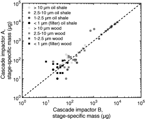
There are two outliers in the 2.5–10 µm size range for oil shale samples. The particulate mass collected was much larger for PM10 B than for PM10 A—this is most likely due to the inlet nozzle of PM10 A being misaligned. There were also a few human errors during the process of taking out the foils and weighing them. The filter stage stuck to its container very easily, and often had to be carefully scraped off. The weighing room was also quite windy due to the air exchanger, which caused challenges when handling the foils and filters. Despite these challenges, the overall results for the PM10 cascade impactor comparison were very good: R² = 0.986.

Figure 5 shows averaged flue gas particle size distributions measured with ELPI+, for electric current (diffusion corrected), particle number and particulate mass. The oil shale and wood combustion cases have been separated, as the particle concentrations were vastly different. The current distributions are nearly identical, whereas there are slight differences in number distributions in the small particle range and notable differences in the mass concentration of large particles. In each distribution plot, the particle mode is at the same particle size.

Figure 5. Comparison of the electric current, particle number concentration and particle mass concentration size distributions as measured by ELPI + A and ELPI + B. The left column is the average of the oil shale emission measurement samples (excluding sample six) and the right column is the average of the wood emission measurement samples. The separate distributions for each sample can be found in Figures S1–S3.

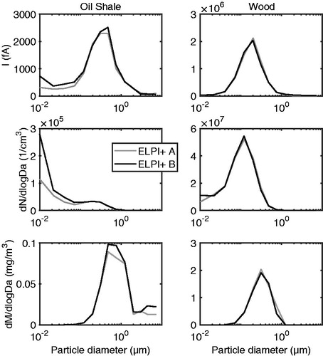
In both combustion cases, ELPI + B reports a higher number concentration of the smallest measured particles. This is true for each separate measurement as well, as can be seen from the raw current results in Figure S1. For the mass concentrations, there is a difference in the largest particle sizes. Again, the ELPI + B consistently reported a larger mass in the larger particle sizes. ELPI + B experienced an error during the measurement of sample 6, and the sample has been excluded from these results. The number and mass distributions are plotted separately in supplementary Figures S2 and S3.

The R² value was over 0.98 for current measured from stages 3 to 8. For the small particle stages the correlation was slightly worse, R² = 0.71 (filter stage) and R² = 0.90 for stage 2. The large particle stages had the lowest correlation values, of only R² = 0.09 for stage 12 and 0.38–0.97 for the others. The reason stage 12 had such poor correlation is that it received almost no current.

To compare the total particle mass concentration reported by each ELPI + to the other instruments, any mass measured from a stage which received less than 2.5% of the total current (after correcting the current for secondary collection effects) was ignored. Although the measured mass in these higher stages can be large, it results from a very small current. Over all 18 measurement cases, stages 10–14 contributed an average of 6.2% of the total current to ELPI + A and 7.3% of the total current to ELPI + B. For the wood cases (7–18), this percentage drops even further, to 1.0% and 2.7% (ELPI + A and ELPI + B). The error margins in the higher stages are quite large due to secondary collection of small particles, which the correction may not adequately account for. For stage 10, the correction (applied by the ELPI + datasheet) was approximately 40% of the measured current, and it is even larger for the higher stages.

3.2. Comparison of electrical measurements

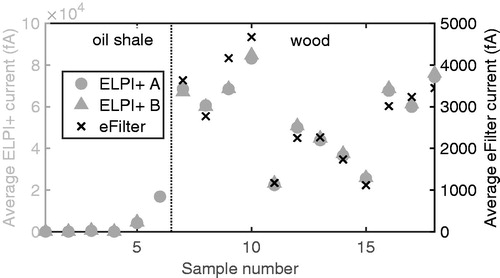
Figure 6 displays the average of the total electric current during each sample as measured by ELPI + A, ELPI + B and eFilter. For ELPI+, the reported current is the sum of all the stages (averaged over the sampling period). The eFilter current is the average of the current over the sampling period. The correlation between the ELPI + instruments is y = 1.00x + 409, R² = 0.999; there is a very small difference in the reported total current, with ELPI + B consistently giving a slightly larger value. The eFilter current is very close to the ELPI + current if adjusted for the different flowrate, correlation curve being y = 0.053x − 128.4, R² = 0.875, compared to ELPI + A. Figure S4 shows the time series data of the electrical current for each measurement sample.

Figure 6. Average measured electric current for ELPI + A, ELPI + B and eFilter at each sample point. These values have not been dilution corrected, as the dilution was the same for all three instruments. Sample 6 has been excluded for ELPI + B due to an error during the measurement.

3.3. Comparison of mass measurements

Figure 7 shows the particle mass concentration calculated from PM10 cascade impactor and eFilter measurements for the wood combustion cases. The oil shale cases have been left out, as the eFilter was not used in these measurements and the results for the PM10 impactors are shown in Figure 8. Only the particle mass concentration up to 10 µm particles is included for the PM10 impactors, in order to leave out any cyclone effects. The eFilter results compare well (less than 21% difference, R² = 0.78 and 0.77, respectively for comparison to PM10 A and B) with the PM10 results for the four pure wood combustion cases (7–10), the results are lower (−24% to −31%) for the wood and waste combustion cases (13 and 14), and higher (+39% to +89%) for the wood and soot remover cases (15–18). The vertical lines show when the filter in the eFilter was exchanged. For example, the particle mass concentration for sample periods 7 and 8 are reported from just one weighed filter, combined with the electric current data. Samples 15 and 16 show that in the eFilter, even relatively small changes in particle mass concentrations can be detected, even when the filter is not changed between the measurements.

Figure 7. The flue gas particle mass concentration measured for each sample by the PM10 cascade impactors and eFilter. The vertical lines show when the eFilter collection filter was changed. Points 11 and 12 are excluded from the eFilter results, as the ejector diluter was partially blocked.

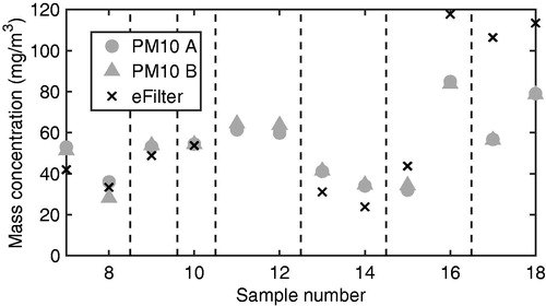
Figure 8. The flue gas particle mass concentration measured by each studied instrument for the 18 sample cases. The dotted vertical line separates oil shale and wood combustion samples. Sample 6 for ELPI + B has been excluded due to an instrument error, other missing points are due to sampling errors (ELPI + A and B, eFilter), or negative mass (PM10 A and B).

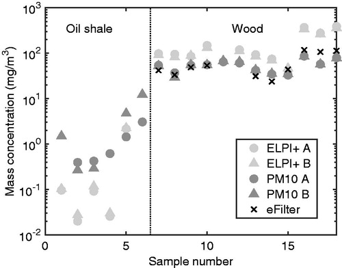
Figure 8 shows the particle mass concentration from each of the studied instruments for each sampling period. The particle mass concentration measured by ELPI+ (A and B) only includes stages which contributed at least 2.5% of the total electrical current, as discussed previously (Section 3.1). In the oil shale combustion cases (samples 1–6); the average results from ELPI + were 26% of the PM10 cascade impactor masses. For the wood combustion cases (7–18) the average ELPI + result is 272% compared to PM10, with the ELPI + instruments reporting values that are 1.4–6.3 times larger than the PM10 reported values. The eFilter results are closer to PM10 values than ELPI+. The results between similar instruments are very consistent. The PM10 impactors vary somewhat in the oil shale case, where particle mass concentrations are small, but ELPI+’s are nearly identical throughout all samples (R² = 0.995).

4. Discussion

Using the PM10 cascade impactors in emission measurements gave nearly identical results. As was seen in Figure 4, the largest deviations were generally in the smallest collected particulate masses, due to the precision of the scale used to weigh the samples. To avoid small masses, low particle concentrations (such as in the oil shale cases, <0.1 mg/m³) need long collection times. This leads to a loss in time resolution, and may even be impossible in cases where the particle production does not last long enough, or the particle source strength varies in time. The correlation for collected mass above 150 µg had much less variance (), compared to smaller particulate masses (). The correlation is even better overall (R² = 0.997), if the points where the inlet may have been misaligned are excluded, showing the importance of the sampling nozzle orientation. Additionally, without a comparison instrument, this error would have gone unnoticed. This highlights the importance of parallel measurements with similar instruments, each with their own inlet.

The electrical current distributions measured by the two ELPI + devices were well correlated for both combustion types, as seen in Figure 5. The correlation was especially good in the wood case. The particle number concentration distributions varied slightly, with ELPI + B consistently showing a slightly larger value in the smaller particle size range, and similarly the mass distribution in the larger particle stages. The small discrepancies between ELPI + A and B in the large and small size ranges indicate a small difference between the instruments, or in the measurement methods employed by research groups A and B; however, the R² was greater than 0.98 for current from most stages and R² = 0.995 for the resulting total mass, meaning that overall the results compared well.

Figure 6 displays the average current measured during each sample by ELPI + A, ELPI + B and eFilter. There was almost no difference between the time-averaged total currents of the two ELPI + instruments (R² = 0.999). The eFilter charging efficiency seems to be similar to the ELPI+, as the measured current was very similar after correcting for the different flow rates between the two instruments (R² = 0.875 and 0.900, respectively for comparison to ELPI + A and B). The particle charge applied by the ELPI + charger has been previously measured to be dependent on for particles smaller than 1 µm (Järvinen et al. 2014). Changes in the eFilter current as compared to ELPI + seem to be caused by a poorly zeroed electrometer. This can be seen from Figure S4, where the eFilter to ELPI + measured current ratio changes during the sampling period in samples 9, 10, and 18. Electrometer drift can be minimized by allowing the instrument more time to warm up, and by checking that the zero level does not change while measuring clean air. As the electrometer drift can play a role in calculating the results, it would be beneficial to record the data also from the zeroing time period. Unfortunately, the zeroing measurements were not recorded for later investigation. There are no previous studies regarding the eFilter, and only one device was available for this study, so we cannot comment on how typical the results are.

As seen in Figure 8, particle mass concentrations calculated from ELPI + are smaller than the PM10 cascade impactor results for oil shale, but 1.3–4.8 times larger when compared to the PM10 results in the wood combustion cases, even when higher stages are excluded, as described in Section 3.1. The ELPI + sample was diluted with one ejector diluter in the oil shale case and with a double ejector in the wood case. These results could have indicated that the difference might be caused by effects from dilution; however, the eFilter results for particle mass concentration had a reasonably good correlation with the PM10 impactor results (R² = 0.78), even though it measured the same diluted flue gas as the ELPI + instruments. As both ELPI + instruments showed similarly high particle mass concentrations, it is evident that the instruments were working as intended. The deviation of the mass concentration results compared to the results from other instruments was highest in the final three measurement cases, in which wood was burned along with the soot remover. However, also the eFilter showed higher particle mass concentrations than the cascade impactors in these three cases, suggesting dilution might have played a partial role. Figure S5 shows ELPI + particle number distributions compared to SMPS distributions. The SMPS results are only indicative, as one measurement cycle is 3 min, which was far too long for these measurements. However, the shapes of the particle number distributions (from ELPI + and SMPS) were similar, and the largest differences were observed in the small particle size range, which does not contribute significantly to the PM.

Previous studies have also indicated higher particle mass concentration results with ELPI + and its predecessor ELPI, when compared to filter collection. Maricq, Xu, and Chase (2006) found that ELPI over-estimated mass and reported several concerns regarding ELPI mass measurements from diesel emissions. Two of these concerns are applicable to the results presented in this article. First, the particle loading effect, which can change the impactor jet geometry due to the accumulation of particles in the jets. Second, Maricq et al. discuss the role of density, and show how a non-constant density can be used to obtain better results. In this study, the particle loading effect was minimized by wiping the jet plates with a cloth and chancing the foils after each measurement day. The mass calculation from ELPI + results would have been improved by taking into account the non-constant density of the particles. In our study, adjustments for density were not made during data processing, as the size-specific density could not be reliably calculated from the available data. Using the SMPS and ELPI + data together, we calculated the densities for the wood combustion measurements to be between 0.7 and 3.8 g/cm³ (Table S3). Leskinen et al. report a range of 0.25–2 g/cm³ for particles from wood combustion emissions, depending on particle size and the burning phase the particles were emitted from (2014). In addition, it should be noted that other studies have found that the assumed (constant) density of particles had a minor effect on the overall particle mass concentration reported by ELPI (Charvet et al. 2015; Moisio 1999).

Hitzenberger et al. (2004) measured PM_2.5 in ambient air and noticed that ELPI gave a mass concentration 1.92 times higher than the average of other measurement methods. They speculated that the cause was moisture in ambient air, as the aerosol was not dried before measuring with ELPI. As we used ELPI + current data to calculate particulate mass, and did not weigh the collected particulate mass from the impactor stages, the sample conditioning can affect the ELPI + results. In our measurements, the raw flue gas was highly diluted (dilution ratio over 80 in the wood combustion cases), thus it is unlikely that the humidity of the flue gas played any role in the ELPI + results. Hitzenberger et al. also speculate that the online measurement by ELPI included semi-volatile compounds, whereas semi-volatile compounds evaporate from filter samples before weighing. Thus, the mass of the nonvolatile PM can be lower than the calculated PM from ELPI + data. The volatility of particles was not measured in our study, and their role remains an uncertainty. In future measurements, we would recommend removing the volatile particle fraction by using a thermodenuder or a hot double ejector diluter system, if the aim of the study is related to nonvolatile/solid particle characterization.

A wood combustion literature review by Obaidullah et al. (2012) gives the typical range of particle number concentrations as particles/cm³. The particle number concentrations calculated from ELPI + in our study were well within this range, with an average of particles/cm³. PM10 concentrations are also reported by Obaidullah et al., ranging from 13 to 67 , measured from filter samples. In our study, the PM10 cascade impactor and eFilter results are of similar magnitude, while the ELPI + results are considerably larger, even when discounting higher stages. Oil shale combustion emissions have been studied for pulverized fuel boilers (Aunela-Tapola, Frandsen, and Häsänen 1998; Häsänen et al. 1997). In their study, the average emission factor for pulverized oil shale combustion was 1100 mg/MJ. Since then, many pulverized fuel power plants have been upgraded and CFB boilers have been built in new power plants (Parve et al. 2011).

In addition to the operation principles, the instruments have some physical differences as well. The ELPI + is the most sophisticated of the three instruments, but it is also the largest. The PM10 cascade impactors and the eFilter are closer in size, but the eFilter offers the advantage of real-time data (as does the ELPI+). This is useful for following trends in combustion, and it can help with detecting problems related to the boiler operation or instrument operation. On the other hand, the PM10 is very robust and can withstand high temperatures, allowing particle collection without dilution. Each of the three instruments requires a separate pump for operation. The eFilter flowrate does not need to be exact, as long as it is approximately constant. The PM10 impactor and ELPI + require a specific flowrate to ensure the impaction of the particles to the correct collection plates. The ELPI + sample flowrate can easily be adjusted with a valve within the instrument, whereas the PM10 impactor requires an additional flow controller. While conducting the measurements, the PM10 impactor requires the most attention from the user. Preparation of the foils is similar between ELPI + and PM10 impactors, but the PM10 foils need baking and weighing before assembling the impactor. After the measurement, the process of taking out the collection foils and weighing them needs to be done very carefully to avoid removing (or adding) mass. The ELPI + produces the highest amount of data, since it gives information about the particle current and number size distribution once every second. The ELPI + can be processed with the software provided with the instrument or with user’s own software. Where the ELPI + data has detailed information about the particle number distribution, the eFilter only gives the current imparted by the particles in the sample flow. To use the eFilter efficiently, weighing the filter to gain information about the collected mass is necessary. The analysis of the results is always left to the user. The least laborious data processing is with the PM10 impactor.

To summarize the major points in this discussion, the particle number and mass concentration in the wood combustion cases was much larger than in the oil shale combustion cases. In all cases, electrical signals were very well correlated and mass concentrations were well correlated for the PM10 impactors and the eFilter, whereas the ELPI + mass concentrations were significantly larger for almost every case. Our hypothesis for this discrepancy is a) the effective density of the particles was not the assumed value of 1 , and b) volatile particles were measured by ELPI+, but were not measured from the filter samples, as volatile compounds would have evaporated before the weighing. A better comparison between instruments could have been made by adding a thermodenuder before the ELPI + instruments and by measuring the effective density by some other means. The eFilter average current correlated well with the ELPI + current in these measurements. When the current signals for the two different instruments were adjusted by the respective flow rates, they matched almost exactly, showing that the eFilter charger efficiency is similar to that of the ELPI+. Comparing the eFilter mass concentration to the PM10 mass concentration showed that the measurement method introduced in the eFilter is valid.

5. Conclusions

Our study shows that the PM10 gravimetric cascade impactor and ELPI + are highly comparable, in that the two different instruments produce the same results, even when operated by different research groups. ELPI + or eFilter is a good alternative to offline measurement methods, when measuring a transient source, as they give data with a 1-s time resolution. To measure particle mass concentration from an emission source, eFilter or a PM10 impactor is generally a better choice, whereas ELPI + is well suited for particle number concentration and size distribution measurements.

The eFilter was shown to have the advantage of real-time current measurement which is comparable to ELPI+, combined with mass concentration results that are comparable to the results from PM10 cascade impactors. In addition, the eFilter requires less attendance (than the PM10 impactor) by the operator during the measurements, as the online current measurement can be used to calculate the approximate particulate mass concentration for any time period. For these reasons, it is a convenient new instrument for emission measurements.

Additional information

Funding

This work was supported by the Estonian Environmental Investment Centre project no. 10627.

References

- “Air Quality Standards.” 2017 European Commission. 2017. Accessed September 6, 2018. http://ec.europa.eu/environment/air/quality/standards.htm.
- Amaral, S., J. de Carvalho, M. Costa, and C. Pinheiro. 2015. An overview of particulate matter measurement instruments. Atmosphere 6 (9):1327–1345. doi:10.3390/atmos6091327.
- Andreae, M. O., C. D. Jones, and P. M. Cox. 2005. Strong present-day aerosol cooling implies a hot future. Nature 435 (7046):1187–1190. doi:10.1038/nature03671.
- Aunela-Tapola, L. A., F. J. Frandsen, and E. K. Häsänen. 1998. Trace metal emissions from the estonian oil shale fired power plant. Fuel Processing Technol. 57 (1):1–24. doi:10.1016/S0378-3820(98)00069-1.
- Brachert, L., J. Mertens, P. Khakharia, and K. Schaber. 2014. The challenge of measuring sulfuric acid aerosols: Number concentration and size evaluation using a condensation particle counter (CPC) and an electrical low pressure impactor (ELPI+). J. Aerosol Sci. 67:21–27. doi:10.1016/j.jaerosci.2013.09.006.
- Burtscher, H. 2005. Physical characterization of particulate emissions from diesel engines: A review. Aerosol Sci. 36 (7):896–932.
- Charvet, A., S. Bau, D. Bémer, and D. Thomas. 2015. On the importance of density in ELPI data Post-Treatment. Aerosol Sci. Technol. 49 (12):1263–1270. doi:10.1080/02786826.2015.1117568.
- Dhaniyala, S., M. Fierz, J. Keskinen, and M. Marjamäki. 2011. Instruments based on electrical detection of aerosols. In Aerosol Measurement: Principles, Techniques, and Applications, ed. Pramod Kulkarni, Paul A. Baron and Klaus Willeke, 393–416. 3rd ed. New York: John Wiley & Sons, Inc. doi:10.1002/9781118001684.ch18.
- Duan, J., J. Tan, S. Wang, J. Hao, and F. Chai. 2012. Size distributions and sources of elements in particulate matter at curbside, Urban and rural sites in beijing. J. Environ. Sci. 24 (1):87–94. doi:10.1016/S1001-0742(11)60731-6.
- Häsänen, E., L. Aunela-Tapola, V. Kinnunen, K. Larjava, A. Mehtonen, T. Salmikangas, J. Leskelä, and J. Loosaar. 1997. Emission factors and annual emissions of bulk and trace elements from oil shale fueled power plants. Sci. Total Environ. 198 (1):1–12. doi:10.1016/S0048-9697(97)05432-6.
- Hering, S. V. 1995. “Impactors, cyclones, and other inertial and gravitational collectors.” In Air sampling instruments for evaluation of atmospheric contaminants, ed. B. S. Cohen and S. V. Hering, 279–321, 8th ed. Ohio: ACGIH.
- Hitzenberger, R. M., A. Berner, Z. Galambos, W. Maenhaut, J. Cafmeyer, J. Schwarz, and K. Müller. 2004. Intercomparison of methods to measure the mass concentration of the atmospheric aerosol during INTERCOMP2000 - Influence of instrumentation and size cuts. Atmos. Environ. 38 (38): 6467–6476. doi: 10.1016/j.atmosenv.2004.08.025.
- Järvinen, A., M. Aitomaa, A. Rostedt, J. Keskinen, and J. Yli-Ojanperä. 2014. Calibration of the new electrical low pressure impactor (ELPI+). J. Aerosol. Sci. 69 (March):150–159. doi:10.1016/J.JAEROSCI.2013.12.006.
- Keskinen, J., K. Pietarinen, and M. Lehtimäki. 1992. Electrical low pressure impactor. J. Aerosol Sci. 23 (4):353–360.
- Koch, W., H. Lödding, W. Mölter, and F. Munzinger. 1988. Verdünnungssystem für die messung hochkonzentrierter aerosole mit optischen partikelzählern. Staub. Reinhaltung Der Luft 48 (9):341–344.
- Konist, A., O. Järvik, T. Pihu, and D. Neshumayev. 2018. Combustion as a possible solution pyrolytic wastewater utilization. Chem. Eng. Trans. 70:859–864. doi: 10.3303/CET1870144.
- Konist, A., B. Maaten, L. Loo, D. Neshumayev, and T. Pihu. 2016. Mineral sequestration of Co2 by carbonation of Ca-Rich oil shale ash in natural conditions. Oil Shale 33 (3):248–259. doi:10.3176/oil.2016.3.04.
- Lee, L. A., C. L. Reddington, and K. S. Carslaw. 2016. On the relationship between aerosol model uncertainty and radiative forcing uncertainty. Proc. Nat. Acad. Sci. 113 (21):5820–5827. doi:10.1073/pnas.1507050113.
- Lelieveld, J., J. S. Evans, M. Fnais, D. Giannadaki, and A. Pozzer. 2015. The contribution of outdoor air pollution sources to premature mortality on a global scale. Nature 525 (7569):367–371. doi:10.1038/nature15371.
- Leskinen, J., M. Ihalainen, T. Torvela, M. Kortelainen, H. Lamberg, P. Tiitta, and G. Jakobi. 2014. Effective density and morphology of particles emitted from small-scale combustion of various wood fuels. Environ. Sci. Technol. 48 (22):13298–13306. doi:10.1021/es502214a.
- Lipsky, E. M., and A. L. Robinson. 2006. Effects of dilution on fine particle mass and partitioning of semivolatile organics in diesel exhaust and wood smoke. Environ. Sci. Technol. 40 (1):155–162. doi:10.1021/es050319p.
- Liu, Z., Y. Ge, K. C. Johnson, A. N. Shah, J. Tan, C. Wang, and L. Yu. 2011. Real-World operation conditions and on-Road emissions of beijing diesel buses measured by using portable emission measurement system and electric Low-Pressure impactor. Sci. Total Environ. 409 (8):1476–1480. doi:10.1016/j.scitotenv.2010.12.042.
- Maricq, M. M., D. H. Podsiadlik, and R. E. Chase. 2000. Size distributions of motor vehicle exhaust PM: A comparison between ELPI and SMPS measurements. Aerosol Sci. Technol. 33 (3):239–260. doi:10.1080/027868200416231.
- Maricq, M. M., N. Xu, and R. E. Chase. 2006. Measuring particulate mass emissions with the electrical low pressure impactor. Aerosol Sci. Technol. 40 (1):68–79. doi:10.1080/02786820500466591.
- Marjamäki, M.,. J. Keskinen, D.-R. Chen, and D. Y. H. Pui. 2000. Performance evaluation of the electrical Low-Pressure impactor. J. Aerosol Sci. 31 (2): 249–261. doi: 10.1016/S0021-8502(99)00052-X.
- Moisio, M. 1999. Real-time size distribution measurement of combustion aerosols. Tampere University of Technology.
- Obaidullah, M., S. Bram, V. K. Verma, and J. De Ruyck. 2012. A review on particle emissions from small scale biomass combustion. Int. J. Renew. Energy Res. 2 (1):147–159. http://www.ijrer.net/index.php/ijrer/article/view/147.
- Parve, T., J. Loosaar, M. Mahhov, and A. Konist. 2011. Emission of fine particulates from oil shale fired large boilers. Oil Shale 28 (1S):152–161. doi:10.3176/oil.2011.1S.07.
- Petzold, A., R. Marsh, M. Johnson, M. Miller, Y. Sevcenco, D. Delhaye, A. Ibrahim., et al. 2011. Evaluation of methods for measuring particulate matter emissions from gas turbines. Environ. Sci. Technol. 45 (8):3562–3568. doi:10.1021/es103969v.
- Pirjola, L., T. Rönkkö, E. Saukko, H. Parviainen, A. Malinen, J. Alanen, and H. Saveljeff. 2017. Exhaust emissions of Non-Road mobile machine: Real-World and laboratory studies with diesel and HVO fuels. Fuel 202:154–164. doi:10.1016/j.fuel.2017.04.029.
- Rönkkö, T., A. Virtanen, K. Vaaraslahti, J. Keskinen, L. Pirjola, and M. Lappi. 2006. Effect of dilution conditions and driving parameters on nucleation mode particles in diesel exhaust: Laboratory and on-Road study. Atmos. Environ. 40 (16):2893–2901. doi:10.1016/j.atmosenv.2006.01.002.
- Virtanen, A., M. Marjamäki, J. Ristimäki, and J. Keskinen. 2001. Fine particle losses in electrical low-pressure impactor. J. Aerosol Sci. 32 (3):389–401. doi:10.1016/S0021-8502(00)00087-2.
- Xue, J., Y. Li, X. Wang, T. D. Durbin, K. C. Johnson, G. Karavalakis, A. Asa-Awuku, M. Villela, D. Quiros, S. Hu, T. Huai, A. Ayala, and H. S. Jung. 2015. Comparison of vehicle exhaust particle size distributions measured by SMPS and EEPS during steady-state conditions. Aerosol Sci. Technol. 49 (10):984–996. doi:10.1080/02786826.2015.1088146.