Optimizing the performance of aerosol photoacoustic cells using a finite element model. Part 1: Method validation and application to single-resonator multipass cells

Abstract

Photoacoustic spectroscopy is the technique-of-choice for non-contact and in situ measurements of light absorption coefficients for aerosols. For most aerosol photoacoustic (PA) detectors, a key process is the amplification of the acoustic pressure wave generated from light absorption through excitation of a pressure eigenmode of a PA cell. To our knowledge, no modeling of the acoustics, sensitivity or signal-to-background ratio (SBR) has been performed for the PA cells applied commonly to aerosol absorption measurements. In this Part 1 manuscript, we develop a finite element method (FEM) framework to simulate the acoustic response and SBR of photoacoustic cells. Furthermore, we validate this modeling framework by comparing FEM predictions of single-resonator PA cells with measurements using a prototype single-resonator cell, the geometry of which can be readily adjusted. Indeed, single-resonator cells are applied commonly to aerosol absorption measurements. We show that our model predicts accurately the trends in acoustic properties with changes to cell geometry. We investigate how common geometric features, used to suppress detection of background and noise processes, impact on the SBR of single-resonator PA cells. Such features include using multiple acoustic buffer volumes and tunable air columns. The FEM model and measurements described in this article provide the foundation of a companion paper that reports the acoustic properties and optimization of a two-resonator PA cell used commonly in aerosol research.

1. Introduction

The interaction of light with aerosol particles in the atmosphere represents one of the largest uncertainties in current climate models, influencing predictions of temperature, cloud cover, and precipitation on global and regional scales (IPCC 2013; Haywood and Boucher 2000). Atmospheric aerosol scatter and absorb solar and terrestrial radiation, causing net cooling or heating effects. The aerosol-light interaction is governed by the aerosol extinction coefficient (α_ext) and how extinction partitions into respective scattering (α_sca) and absorption (α_abs) contributions, with α_ext = α_sca + α_abs (Haywood and Shine 1995). Reducing the uncertainties associated with aerosol-light interactions necessitates improved in situ instrumentation for measuring α_ext, α_sca, and α_abs accurately and sensitively.

Established techniques such as cavity ring-down spectroscopy (Cotterell et al. 2016, 2017; Langridge et al. 2011; Miles et al. 2011; Lang-Yona et al. 2010) and nephelometry (Sharma et al. 2013; Massoli et al. 2009; Anderson et al. 2003) measure aerosol extinction and scattering, respectively, in a non-contact manner and are used routinely for atmospheric measurements. However, non-contact techniques for measuring aerosol absorption directly are not commonplace for either laboratory studies of aerosol or measurements performed in the field, particularly from research aircraft platforms. The lack of accurate measurements of aerosol absorption coefficients is a key factor limiting the development of accurate aerosol light absorption schemes used in climate models (Stier et al. 2007) and improved spectroscopic methods are needed. Most commonly, researchers characterize aerosol absorption by collecting aerosol on a filter through which the transmission of laser light is measured and the resulting attenuation is related to α_abs. Researchers have reported biases in the retrieved α_abs from filter-based measurements over the range 20–80% (Davies et al. 2019; Cappa et al. 2008; Lack et al. 2008; Bond, Anderson, and Campbell 1999). These biases are attributed to several processes that include the modification of the filter substrate by liquid aerosol components, changes in the aerosol structure and size upon impaction (e.g., from the redistribution of organic components and the aggregation of particles), and multiple scattering interactions.

Photoacoustic spectroscopy (PAS) measures aerosol absorption coefficients for an aerosol sample in a non-contact manner for aerosol in its natural suspended state. Deferring a full explanation of PAS to Section 2, the technique is based upon detection of the periodic pressure wave generated by continuous cycles of laser-induced aerosol heating. This periodic pressure wave results from particles liberating their heat to surrounding gas molecules through collisional quenching and the gas undergoing adiabatic cycles of thermal expansion/contraction at the laser modulation frequency. A photoacoustic cell (PA cell) amplifies the pressure wave for detection by a sensitive microphone, with the amplitude of the microphone response directly proportional to the aerosol absorption coefficient. PAS is well established in trace gas detection applications (Risser et al. 2015; Lindley et al. 2007; Bijnen, Reuss, and Harren 1996; Brand et al. 1995) and a growing number of researchers are using PAS routinely for aerosol absorption measurements in both field (Davies et al. 2019; Peers et al. 2019; Lack et al. 2012; Krämer, Bozoki, and Niessner 2001; Arnott et al. 1999) and laboratory (Cotterell et al. 2019a; Davies et al. 2018; Bluvshtein et al. 2017; Cremer et al. 2016; Haisch et al. 2012) studies. Although PAS has limitations in studying particles with volatile components (Diveky et al. 2019; Langridge et al. 2013) and particles with diameters larger than 1 µm (Cremer et al. 2017; Sedlacek and Lee 2007), PAS has emerged as the technique-of-choice for high accuracy in situ and non-contact measurements of aerosol α_abs.

A key aspect to the PAS detection process is the amplification of the aforementioned periodic pressure wave by the PA cell. Figure 1a shows the general structure of a single-resonator PA cell with a resonator pipe connecting two volumes referred to as acoustic buffers. The cell is an acoustic resonator, with periodic pressure waves coupling into a resonant mode of the cell if the frequencies of pressure waves match that of the resonant mode. A typical cell consists of one or two cylindrical resonator pipers capped by acoustic buffers. Lack et al. (2012) assessed the sensitivities and uncertainties in aerosol α_abs using their PA cell, consisting of two resonator pipes of radii ∼1 cm capped by acoustic buffers. From measurements of the microphone response over 1-s intervals, the sensitivity in α_abs was determined to lie in the range of 0.5–1.5 ${\mathrm{Mm}}^{-1},$ with an uncertainty and accuracy of ∼10% for α_abs measurements performed from an aircraft platform. The PAS measurements contained large levels of noise compared to in-flight measurements of extinction coefficients from cavity ring-down spectroscopy that had 1-s detection limits and accuracies better than 0.1 ${\mathrm{Mm}}^{-1}$ and 2%, respectively (Langridge et al. 2011). Therefore, while PAS measurements of α_abs remain the most precise and accurate values available, the performance is not yet reaching the levels attained by alternative spectroscopic techniques measuring extinction.

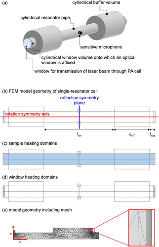
Figure 1. (a) The general structure and features of a single-resonator cell. (b) The two-dimensional axisymmetric model geometry used to represent our cell in FEM calculations. (c) The sample heating domains are highlighted. (d) The window heating domains are highlighted. (e) The meshed geometry solved in our model. The inset shows an expanded portion of this mesh near the cell surface to highlight the dense boundary layer mesh for resolving thermal and viscous damping. Also indicated are the longitudinal (z) and radial (r) coordinate axes.

The dominant uncertainty in α_abs arises from background noise contributions to the measured microphone response caused by interactions of the laser beam with the entrance and exit windows of the PA cell (Lack et al. 2012; Miklós, Hess, and Bozóki 2001; Bijnen, Reuss, and Harren 1996). Laser-window interactions occur through either light scattering, where photon momentum is transferred to the window surface causing mechanical vibrations that generate pressure waves, or through heating the window surfaces via light absorption that creates an additional photoacoustic source. The high background levels necessitate a background subtraction procedure in post-processing of photoacoustic measurements. Moreover, field measurements made aboard aircraft demonstrate a strong dependence of the window background on pressure (Lack et al. 2012), with the pressure varying from 1000 to 400 hPa as the altitude increases from ground level to ∼9 km, further complicating the background subtraction procedure. Lack et al. (2012) estimate that this background subtraction process introduces at least a 0.5 ${\mathrm{Mm}}^{-1}$ uncertainty. In our own research, we develop robust and sensitive PAS instruments to measure aerosol absorption coefficients from an airborne research platform (the UK research aircraft, FAAM BAe-146) (Davies et al. 2019; Peers et al. 2019) in addition to laboratory studies of aerosol (Cotterell et al. 2019a; Davies et al. 2018). In the Part 2 paper (Cotterell et al. 2019), we show that we measure the same level of degradation in absorption sensitivity caused by laser-window interactions as those reported by Lack et al. (2012) using the same PAS cell from the NOAA WP-3D aircraft. Consequently, the geometry of the photoacoustic cell should be optimized such that the desired signal from aerosol sample absorption is amplified as much as possible, with pressure waves coupling into an acoustic resonance (eigenmode) of the cell. Simultaneously, the cell should be insensitive to pressure couplings corresponding to background sources, such as laser-window interactions.

While much attention has been given to the design of PA cells for trace gas detection, little consideration has been given to optimizing cell geometries for aerosol absorption measurements. For trace gas detection cells, the resonator pipes are often narrow (diameter <5 mm) with a single pass of the excitation laser source through the resonator pipe center (Sadiek et al. 2018; Risser et al. 2015; Parvitte et al. 2013; Lindley et al. 2007; Bijnen, Reuss, and Harren 1996). However, the distribution of aerosol particles in ambient samples are discrete and non-uniform, with number concentrations often low (<100 ${\mathrm{cm}}^{-3}$). Thus, to measure photoacoustic signals sensitively for aerosols, either very high laser powers (approx. >1 W) are required or a low power laser beam (<100 mW) is reflected back and forth through the aerosol sample (Nägele and Sigrist 2000). It has become commonplace for a typical aerosol PAS detector to use a low power laser beam coupled into an astigmatic optical cavity. Here, the laser beam is reflected back and forth through the aerosol-laden sample such that the reflected beam never retraces the incident beam, increasing the intra-cavity power in addition to the beam path length and detection volume (Cotterell et al. 2019a; Fischer and Smith 2018a; Davies et al. 2018; Bluvshtein et al. 2017; Lack et al. 2012; McManus, Kebabian, and Zahniser 1995), while providing low levels of heating to a single particle and thus minimizing the probability of evaporation of semi-volatile components (Lack et al. 2006). The transverse cross-section of this multipass beam thus consists of a pattern of bright spots often distributed over an effective area of ∼1 cm². Due to the requirement for a multipass laser beam configuration, resonator pipe diameters in aerosol cells are typically ∼2 cm. While researchers have studied the geometry optimization of cells with narrow resonator diameters, it is unclear whether such studies are relevant to multipass cells applied commonly to aerosol detection. Thus, improved measurements of aerosol absorption coefficients using PAS require geometry optimization studies for multipass PA cells.

1.1. Optimizing the performance of photoacoustic cells

Numerous studies have reported experimental and theoretical investigations of gas PA cell optimization. Using transmission line theory, Bijnen, Reuss, and Harren (1996) reported the optimization of a single-resonator cell for detection of trace gases and verified their model predictions with measurements. The general structure of their PA cell is similar to that analyzed in this work, consisting of a resonator pipe capped by cylindrical buffer volumes and adjoining window volumes, albeit with a much narrower (3–4 mm radius) resonator pipe. The authors established, for the limited set of cell geometries assessed, that large buffer radii suppressed window background contributions while improving the sensitivity. Moreover, the authors investigated the impact of additional cylindrical volumes of variable length connected to the cylindrical face of the window volumes on the window background. These additional volumes, referred to as tunable air columns (TACs), provided effective suppression of the window heating background when the column lengths were equal to half the resonator pipe length. Baumann et al. (2006, 2007) first applied finite element method (FEM) modeling to the analysis of photoacoustic cells; the authors modeled T-shaped cells consisting of a large diameter cylinder through which a laser beam passed, while a microphone located in a coupled narrow pipe detected the amplified PA signal. Reasonable agreement was found between frequency-dependent pressures at the microphone location for FEM predictions and experimental measurements, with this agreement getting progressively worse at higher frequencies (>1000 Hz), suggesting that boundary layer processes associated with thermoviscous effects (see Section 2) that removed acoustic energy were not accounted for adequately. Meanwhile, Risser et al. (2015) and Parvitte et al. (2013) reported near-exact agreement between measurements and FEM predictions for the lowest frequency mode (resonance frequency, f₀ ∼ 600 Hz) of a differential Helmholtz cell, proving that FEM can be used to predict accurately the acoustic properties of PA cells.

While the studies above establish FEM as a useful and accurate tool for predicting the performance of PA cells, they are not of direct relevance to geometries used for aerosol detection. Moreover, the studies focused on modeling acoustic eigenmode distributions and did not extend the use of FEM to investigate how cell design can be optimized to maximize the signal-to-background ratio (SBR), which is ultimately the quantity that governs the PAS detection limit. Therefore, in this Part 1 publication, we report the first rigorous treatment of the thermoviscous acoustics for PA cells with a generic single-resonator geometry that is often used in aerosol α_abs measurement, and develop an FEM modeling framework for assessing the SBR of PA cells for the first time. We apply FEM to model the performance of a simple, single-resonator cell capped by buffer volumes and maximize the SBR by optimizing the cell geometry. Crucially, this Part 1 publication reports validation studies to ensure our modeling framework reliably predicts trends in the key acoustic performance parameters with changes to the PA cell geometry by comparing model predictions with measurements. Importantly, the description and validation of our FEM model for predicting PA cell performance forms the basis of a companion paper (Cotterell et al. 2019b) assessing the acoustics of a two-resonator cell that is applied commonly to aerosol α_abs measurements (Foster et al. 2019; Cotterell et al. 2019a; Fischer and Smith 2018a; Davies et al. 2018; Bluvshtein et al. 2017; Lack et al. 2012). The following section describes important theoretical aspects of thermoviscous acoustics pertinent to this work. Section 3 describes the FEM model we used to simulate the thermoviscous acoustics of a single-resonator cell and the experimental methods used to validate model predictions. Then, Section 4 discusses the geometry optimization of single-resonator cells to maximize the SBR and the influence of multiple buffer volumes and TACs on instrument performance.

2. Photoacoustics in an acoustic cavity

The PA process has been described in detail by Rosencwaig (1980) and Miklós, Hess, and Bozóki (2001). Briefly, intensity modulated laser light is absorbed by a sample through excitation of molecular rotational, vibrational and/or electronic energy levels. For molecular absorption transitions where the fate of excited molecules is dominated by collisional relaxation (and radiative relaxation, photo-dissociation and latent heat energy pathways can be ignored), energy is transferred to translational degrees of freedom of the bath gas. This heat transfer causes thermal expansion and generates a pressure wave, with the magnitude of this pressure wave proportional to the sample absorption coefficient. Central to the PA process is the amplification of the pressure wave through excitation of a PA cell pressure eigenmode, a standing wave solution intrinsic to the cell geometry. In resonant PAS, the laser source is modulated periodically at the resonance frequency (eigenfrequency) corresponding to the cell eigenmode. Repeated cycles of bath gas thermal expansion/contraction generate a periodic pressure wave that couples efficiently into the cell eigenmode, providing there is sufficient spatial overlap between the eigenmode pressure p_n($\overrightarrow{r}$) and the heat deposition H($\overrightarrow{r}$) distributions (see Section 2.2). The eigenmode has an associated quality factor (Q) describing the energy stored in the resonator relative to the energy lost over one complete period. Typically, Q values greater than 50 are found in the literature (Davies et al. 2018; Lack et al. 2012), amplifying the magnitude of the photoacoustic pressure wave by the same factor. This resonant amplification process allows detection of the photoacoustic pressure wave by a sensitive microphone located at an eigenmode pressure maximum within the PA cell. Typically, the magnitude of the pressure response after amplification is on the order of ∼10 µPa and is linearly proportional to α_abs (Lack et al. 2006, 2012; Bijnen, Reuss, and Harren 1996). By calibrating the spectrometer with a species of known absorption (typically a gaseous absorber such as ozone, the concentration of which is verified using an independent calibration-free technique such as cavity ring-down spectroscopy), α_abs is determined from the microphone response (Cotterell et al. 2019a; Fischer and Smith 2018b; Davies et al. 2018).

Amplification of the PA pressure wave by coupling into a cell eigenmode is central to resonant PAS. Understanding this acoustic amplification requires coupled equations for pressure, velocity, and temperature to be solved. We now describe these governing equations for thermoviscous acoustic processes and how they are solved using FEM. Then, we present the general solution of the inhomogeneous Helmholtz equation that will be useful for interpreting our later results.

2.1. The governing equations for thermoviscous acoustic processes

The acoustics of geometries very large compared to the acoustic wavelength are described by the inhomogeneous wave equation. For geometries with dimensions similar to or smaller than the acoustic wavelength, significant energy damping arises from thermal and viscous losses at surfaces and require the thermovisous acoustic equations to be solved. Typical PA cells operated at kilohertz frequencies provide an example of a thermoviscous acoustics problem. Thermoviscous acoustic processes concern perturbations in the three fluid properties of velocity, pressure, and temperature. We require solutions to a set of four equations: the momentum equation, continuity equation, Fourier heat law (relating time-dependent pressure and temperature to heat sources and thermal conductivity), and an equation of state describing the dependence of density on pressure and temperature (COMSOL User’s Guide 2016). The relevant acoustic fields of interest are the small perturbations in velocity ($\overrightarrow{u}$), pressure (p), and temperature (T) against their respective background values (${\overrightarrow{u}}_0,$ p₀, and T₀). Because the fields of interest represent a small perturbation, a small parameter expansion (or linearization) of the four governing equations is performed. Assuming that these small perturbations to the background fields are periodic (time dependence of $e^{i\omega t},$ with ω the angular frequency and t time), the governing equations are: (1) $$i\omega {\rho }_0\overrightarrow{u}=\nabla ·\left[-p\mathbf{I}+\mu \left(\nabla \overrightarrow{u}+{\left(\nabla \overrightarrow{u}\right)}^T\right)-\left(\frac{2\mu }{3}-{\mu }_{\mathrm{B}}\right)\left(\nabla \overrightarrow{u}\right)\mathbf{I}\right]$$(1) (2) $$i\omega \rho +\mathrm{ }{\rho }_0\left(\nabla \overrightarrow{u}\right)=0$$(2) (3) $$i\omega \left({\rho }_0{C}_{p}T-p{T}_0{\alpha }_0\right)=-\nabla \left(-k\nabla T\right)+H$$(3) (4) $$\rho ={\rho }_0\left({\beta }_{T}p-{\alpha }_{0}T\right)$$(4) in which $\rho$ is a small perturbation in the background density ${\rho }_0,$ I is the identity matrix, $\mu$ and ${\mu }_{\mathrm{B}}$ are the dynamic and bulk viscosities, $C_p$ is the specific heat capacity at constant pressure, k is the thermal conductivity, H is the energy deposited, ${\alpha }_0$ is the isobaric coefficient for thermal expansion, and ${\beta }_T$ is the isothermal compressibility (COMSOL User’s Guide 2016). Deriving analytical solutions of the thermoviscous acoustic equations is not possible for most geometries. Therefore, FEM divides a geometry into many small elements using a mesh, with the thermoviscous equations solved numerically for each element and the solutions coupled for adjacent elements by boundary conditions.

2.2. Solutions to the inhomogeneous Helmholtz equation including damping

Although not providing a rigorous solution to the thermoviscous acoustic equations, it is useful to consider the general solution to the inhomogeneous Helmholtz equation. For an ideal gas in the limit of adiabatic expansion (k = 0), neglecting heat sources and assuming that viscosity is negligible, it can be shown that the thermoviscous wave equations reduce to the homogenous Helmholtz equation: (5) $${\nabla }^{2}p\left(\overrightarrow{r}\right)+\frac{{\omega }^2}{c^2}p\left(\overrightarrow{r}\right)=0$$(5) in which $p\left(\overrightarrow{r}\right)$ is the pressure distribution and c is the speed of sound (COMSOL User’s Guide 2016). If the heat source term is not ignored, the inhomogeneous Helmholtz equation is derived: (6) $${\nabla }^{2}p\left(\overrightarrow{r}\right)+\frac{{\omega }^2}{c^2}p\left(\overrightarrow{r}\right)=i\frac{\left(\sigma -1\right)}{c^2}H\left(\overrightarrow{r}\right)$$(6) in which $\sigma$ is the adiabatic coefficient (Miklós, Hess, and Bozóki 2001; Rosencwaig 1980). This equation neglects viscous and thermal damping, but we will subsequently include these losses as a perturbation to the general solution. The general solution to the inhomogeneous wave equation is: (7) $$p\left(\overrightarrow{r}\right)=A_0+\sum _n{A}_n{p}_n\left(\overrightarrow{r}\right)$$(7) with $p_n\left(\overrightarrow{r}\right)$ the eigenmode pressure distribution, A_n the amplitude quantifying the contribution of p_n to the total pressure, and A₀ the background pressure contribution that is not associated with eigenmode excitation and is inversely proportional to frequency. The eigenmode distributions $p_n\left(\overrightarrow{r}\right)$ are solutions to the homogeneous Helmholtz Equation (5)(5) $${\nabla }^{2}p\left(\overrightarrow{r}\right)+\frac{{\omega }^2}{c^2}p\left(\overrightarrow{r}\right)=0$$(5) and represent orthogonal modes of the PA cell: (8) $$\frac{1}{V}\int p_n{p}_{m}dV={\delta }_{\mathit{nm}}$$(8) with V the volume of the cell and ${\delta }_{\mathit{nm}}$ the Dirac delta function. In PAS, we are interested in the pressure amplitude A_n resulting from resonant excitation of an eigenmode. It can be shown that A_n is given by: (9) $$A_n=\frac{i\omega \left(\sigma -1\right)}{\left({\omega }_n^2-{\omega }^2+i\frac{\omega {\omega }_n}{Q_n}\right)}\frac{\int H\left(\overrightarrow{r}\right)p_n\left(\overrightarrow{r}\right)dV}{V}$$(9) in which $\omega$ represents the modulation frequency of the heat source and ${\omega }_n$ is the eigenfrequency (Miklós, Hess, and Bozóki 2001). Here, we have included a term incorporating the quality factor Q_n of the resonance, with a higher Q corresponding to lower damping of acoustic energy and a higher amplification of the photoacoustic pressure. The inclusion of the Q term represents a perturbation to the general solution to incorporate energy losses (e.g., thermal and viscous damping, see below).

In PAS, laser modulation provides a heat source $H\left(\overrightarrow{r}\right)=I_{0}g\left(\overrightarrow{r}\right){\alpha }_{\mathrm{abs}}\left(\overrightarrow{r}\right),$ with I₀ the laser intensity and $g\left(\overrightarrow{r}\right)$ the normalized laser intensity distribution function (e.g., a Gaussian). Therefore, substituting Equation (9)(9) $$A_n=\frac{i\omega \left(\sigma -1\right)}{\left({\omega }_n^2-{\omega }^2+i\frac{\omega {\omega }_n}{Q_n}\right)}\frac{\int H\left(\overrightarrow{r}\right)p_n\left(\overrightarrow{r}\right)dV}{V}$$(9) into (7)(7) $$p\left(\overrightarrow{r}\right)=A_0+\sum _n{A}_n{p}_n\left(\overrightarrow{r}\right)$$(7) and assuming the resonances of interest are at sufficiently high frequency (>500 Hz) that we can neglect A₀, the pressure at the microphone location ($\overrightarrow{r}={\overrightarrow{r}}_M$) in a PA cell is given by: (10) $$p\left({\overrightarrow{r}}_M,\omega \right)=\sum _n\frac{i\omega \left(\sigma -1\right)I_0}{\left({\omega }_n^2-{\omega }^2+i\frac{\omega {\omega }_n}{Q_n}\right)}\frac{\int g\left(\overrightarrow{r}\right){\alpha }_{\mathrm{abs}}\left(\overrightarrow{r}\right)p_n\left(\overrightarrow{r}\right)dV}{V}{p}_n\left({\overrightarrow{r}}_M\right)$$(10)

The microphone response is given by the absolute value of $p\left({\overrightarrow{r}}_M\right)$ which, for the efficient excitation of a single eigenmode, is given by: (11) $$\left|p\left({\overrightarrow{r}}_M,\omega \right)\right|=\frac{\left(\sigma -1\right)I_0{J}_n{p}_n\left({\overrightarrow{r}}_M\right)}{V}\sqrt{\frac{Q_n^2/{\omega }_n^2}{1+Q_n^2{\left(\frac{{\omega }_n}{\omega }-\frac{\omega }{{\omega }_n}\right)}^2}}$$(11)

Here, we have defined an overlap integral $J_n=\int g\left(\overrightarrow{r}\right){\alpha }_{\mathrm{abs}}\left(\overrightarrow{r}\right)p_n\left(\overrightarrow{r}\right)dV$ describing the spatial overlap of the laser beam, absorbing medium and eigenmode pressure distribution. It follows that the frequency-dependent microphone response is of the form: (12) $$\left|p\left({\overrightarrow{r}}_M,\omega \right)\right|=p_0\sqrt{\frac{1}{1+Q_n^2{\left(\frac{{\omega }_n}{\omega }-\frac{\omega }{{\omega }_n}\right)}^2}}$$(12) with p₀ the resonant peak amplitude. However, it is common to use a Lorentzian distribution (Equation (13)(13) $$\left|p\left({\overrightarrow{r}}_M,\omega \right)\right|=p_0\sqrt{\frac{1}{1+{\left(2Q_n\frac{\left(\omega -{\omega }_n\right)}{{\omega }_n}\right)}^2}}$$(13) ) to describe the frequency-dependent microphone response (Arnott et al. 2006; Miklós, Hess, and Bozóki 2001; Schäfer, Miklós, and Hess 1997); fitting either Equation (12)(12) $$\left|p\left({\overrightarrow{r}}_M,\omega \right)\right|=p_0\sqrt{\frac{1}{1+Q_n^2{\left(\frac{{\omega }_n}{\omega }-\frac{\omega }{{\omega }_n}\right)}^2}}$$(12) or (13)(13) $$\left|p\left({\overrightarrow{r}}_M,\omega \right)\right|=p_0\sqrt{\frac{1}{1+{\left(2Q_n\frac{\left(\omega -{\omega }_n\right)}{{\omega }_n}\right)}^2}}$$(13) to a measured resonance gives negligible differences in the best-fit p₀, Q_n, and ${\omega }_n.$ (13) $$\left|p\left({\overrightarrow{r}}_M,\omega \right)\right|=p_0\sqrt{\frac{1}{1+{\left(2Q_n\frac{\left(\omega -{\omega }_n\right)}{{\omega }_n}\right)}^2}}$$(13)

We now consider sources of acoustic damping in a PA cell that contribute to the reduction of Q_n. Sources of damping are classed either as bulk losses (e.g., viscous losses within the bath gas) or as surface losses, with the latter the dominant contribution. Specifically, thermal and viscous boundary layer losses at surfaces govern energy damping in PA cells. The gaseous expansion/contraction process is adiabatic in the bulk but becomes an isothermal process at boundaries as thermal conductivities of solids are many orders of magnitude higher than those of gases. The removal of heat at surfaces reduces the circulating energy in an acoustic eigenmode. Additionally, the acoustic velocities of gas molecules in the bulk are proportional to the acoustic pressure gradient $\nabla p$ (Equation (1)(1) $$i\omega {\rho }_0\overrightarrow{u}=\nabla ·\left[-p\mathbf{I}+\mu \left(\nabla \overrightarrow{u}+{\left(\nabla \overrightarrow{u}\right)}^T\right)-\left(\frac{2\mu }{3}-{\mu }_{\mathrm{B}}\right)\left(\nabla \overrightarrow{u}\right)\mathbf{I}\right]$$(1) ), while the air molecules closest to surfaces can be regarded as having zero tangential components of velocity (i.e., no-slip). The transition in the velocity distribution from the bulk to PA cell surfaces leads to significant viscous energy losses close to these surfaces. Importantly, the characteristic length scales over which thermal and viscous losses occur are given by the thermal and viscous boundary layer thicknesses δ_T and δ_v, respectively, (Arnott et al. 2006): (14) $${\delta }_T=\sqrt{\frac{2k}{C_p\rho \omega }}\mathrm{ },\mathrm{ }{\delta }_v=\sqrt{\frac{2\mu }{\rho \omega }}$$(14) in which k is the thermal conductivity of air. In air, δ_T and δ_v are comparable with respective values of ∼70 and ∼60 µm at 1500 Hz frequency.

3. Experimental and numerical methods

We now describe our finite element model for a single-resonator PA cell that solves the aforementioned thermoviscous Equations (1)–(4) numerically to predict the frequency-dependent microphone response $\left|p\left({\overrightarrow{r}}_M,\omega \right)\right|.$ We then provide details of experiments that measured the acoustic properties of single-resonator PA cells.

3.1. Finite element model for a single-resonator PA cell

We used the FEM modeling software COMSOL Multiphysics 5.2a with the acoustics module. All simulations reported here used the thermoviscous acoustics interface. Figure 1b shows our model geometry to represent a single-resonator cell. The cylindrical resonator section has a length l_res, radius r_res, and is capped by cylindrical acoustic buffer volumes of length l_buf and radius r_buf. Acoustic buffer volumes are a typical feature of PA cells, with their function to suppress detection of laser-window contributions to the microphone signal. Each buffer volume is affixed to a cylindrical window volume with a length l_win = 1.0 cm and radius r_win = 1.0 cm; in a measurement cell, optical windows affix to these window volumes. To reduce computational cost, we applied two symmetry conditions (see Figure 1b). First, a rotation symmetry axis passed through the center of the resonator pipe, buffer and window volumes. This rotation symmetry allowed our geometry to be represented by a two-dimensional axisymmetric model. Second, a reflection symmetry plane was placed through the center of the resonator and orthogonal to the rotation symmetry axis. Figure 1b shows a microphone with a width of 0.5 cm protruding into the resonator pipe by 0.1 cm. Because of the rotational symmetry in our model, the microphone is a ring in three dimensions and is not representative of the geometry of our laboratory PAS instrument (see Section 3.2). The microphone domain only serves to provide a surface over which to evaluate the pressure at the PA cell center. The equilibrium temperature and pressure are set to T₀ = 293.15 K and p₀ = 1013 hPa (i.e., atmospheric pressure) in all simulations. The required properties of air (e.g., µ, ρ₀, C_p, and k) are taken from the built-in material library of COMSOL Multiphysics. We assigned no-slip and isothermal boundary conditions to the internal surfaces of the cell. In measurements, a multi-pass laser beam propagated parallel to the rotational symmetry axis. Figure 1c shows how heat deposited in the cell by this laser beam was represented in our model, by assigning a sample heating domain. The heat deposited H (see Equation (3)(3) $$i\omega \left({\rho }_0{C}_{p}T-p{T}_0{\alpha }_0\right)=-\nabla \left(-k\nabla T\right)+H$$(3) ) was represented by: (15) $$H\left(\overrightarrow{r}\right)=\frac{I_0}{\pi w^2}\exp \left(-\frac{r^2}{2w^2}\right){\alpha }_{\mathrm{abs}}$$(15) in which I₀ is the laser power amplitude, $w$ is the beam waist of a Gaussian beam and r is the radial distance from the rotation symmetry axis. In all simulations of sample heating, we used I₀ = 0.1 W, w = 0.5 mm and a sample absorption coefficient ${\alpha }_{\mathrm{abs}}$ = 5 × 10⁻⁶ m⁻¹, a typical absorption coefficient for low concentrations of light absorbing aerosol in the atmosphere. To calculate SBR, we also need to include sources from background processes. As discussed in the introduction, the dominant contribution to the measured background is most often laser-window interactions. Therefore, Figure 1d shows window heating domains with a thickness of 2 mm (a similar value to window thicknesses used in measurements) and located 1 mm from the boundary of the window volumes. These window heating domains simply facilitate the deposition of heat within the PA cell at a location close to the window volume boundary. With the exception of the absorption coefficient, all other material properties for these window heating domains are prescribed the material properties of air. The heat deposited in these domains is also modeled by Equation (15)(15) $$H\left(\overrightarrow{r}\right)=\frac{I_0}{\pi w^2}\exp \left(-\frac{r^2}{2w^2}\right){\alpha }_{\mathrm{abs}}$$(15) using the same parameters above, albeit using ${\alpha }_{\mathrm{abs}}$ = 0.1653 m⁻¹, i.e., the absorption coefficient for N-BK7 glass at an optical wavelength of 550 nm (www.refractiveindex.info/?shelf=glass&book=BK7&page=SCHOTT, accessed November 2016). We performed our laboratory measurements (see Section 3.1) subsequent to our modeling studies and only UV fused silica windows with an anti-reflective coating were available in measurements. Nonetheless, the absorption coefficient for UV fused silica has been measured as 0.266 m⁻¹ at visible wavelengths and is similar to that of N-BK7 glass (Zhang et al. 2017). In modeling laser-window interactions, we did not include pressure sources to mimic light scattering from the windows as this proved not possible in the COMSOL Multiphysics thermoviscous acoustics interface without perturbing the no-slip and isothermal boundary conditions.

Central to FEM is the careful choice of mesh for resolving physical phenomena suitably; a mesh with a coarse spatial resolution will fail to capture thermal and viscous damping adequately, while a very high resolution mesh results in a computationally expensive model. Figure 1e shows the mesh structure, including both a bulk and boundary layer mesh, with the latter mesh component highlighted in the figure inset. Section SI.1.1. of the Supporting Information (SI) describes the mesh parameters used in our calculations. Importantly, both a bulk and boundary layer mesh are used, with the boundary layer mesh resolving finely the damping effects occurring in the thermal and viscous boundary layers over characteristic length scales δ_T and δ_v.

COMSOL Multiphysics was used to perform eigenfrequency studies, where the eigenmodes p_n($\overrightarrow{r}$) and their associated eigenfrequencies are calculated. Furthermore, frequency domain studies were performed that calculated the frequency-dependent variations in pressure, temperature and the three components of fluid velocity, with acoustic excitation provided by either sample or window heating. We determined the signal and background microphone responses from these frequency domain studies; the microphone responses for either sample heating $\left|p_{\mathrm{sig}}\left({\overrightarrow{r}}_M,\omega \right)\right|$ or window heating $\left|p_{\mathrm{bck}}\left({\overrightarrow{r}}_M,\omega \right)\right|$ excitation were calculated by integrating the absolute pressure over the microphone surface, normalizing for the microphone surface area.

3.2. Experimental measurements of photoacoustic cell performance

Here, we describe the geometry of the PA cell used in our measurements and provide a brief description of the PAS optical system and data processing; the reader is referred to our previous publications for a complete description of the this optical system and data acquisition (Cotterell et al. 2019a; Davies et al. 2018). We manufactured a single-resonator photoacoustic cell that served only as a testbed for studying the influence of the buffer volume diameters on the acoustic properties of the cell. The single-resonator PA cell was manufactured from aluminum alloy (grade 6082). The resonator had a length and radius l_res = 11.2 cm and r_res = 1.1 cm, respectively. We used buffer volumes where the radius of the volumes could be varied. The buffer volumes consisted of an outer housing with l_buf = 5.5 cm and r_buf = 5 cm and cylindrical aluminum inserts to reduce r_buf to values of 2, 3, or 4 cm. The cylindrical window volumes had dimensions l_win = 1.0 cm and r_win = 1.0 cm, to which UV fused silica windows with a broadband anti-reflective coating (Thorlabs, WG41050-A) were fixed. A continuous wave 658 nm wavelength diode laser (130 mW iBeam Smart, Toptica Photonics) was multi-passed through the PA cell ∼50 times within an astigmatic multi-pass optical cavity. The PA cell was located within this optical cavity. The optical cavity consisted of two cylindrical mirrors with their cylindrical axes aligned at 90° with respect to each other. The laser intensity was modulated periodically by direct control of the laser diode current, with this modulation frequency matching that of the PA cell resonance frequency (see below on measurement of this resonance frequency). A photodiode was located behind the rear cavity mirror and measured the RMS laser power. A sensitive microphone (Knowles Acoustics, EK-23132) was located at the center of the PA cell resonator. The detection electronics and processing are described in our previous publication (Davies et al. 2018) and mimics the processing used by Lack et al. (2012). Briefly, the microphone time-domain signal was collected in 1-s intervals and Fourier-transformed to the frequency domain. The microphone response was then calculated by integrating the frequency-domain microphone signal over a 1 Hz range from f_n – 0.5 Hz to f_n + 0.5 Hz, with f_n the eigenfrequency. We refer to this integrated signal as the integrated area (IA). The cell eigenfrequency f_n depends on the cell temperature, which may change as the ambient temperature fluctuates. No active control of the cell temperature was used during the laboratory measurements reported here. Instead, we measured the resonance frequency at regular (every 5 min) intervals by exciting the PA cell using a speaker (Knowles Acoustics, ES-23127-000) that was permanently located at the center of the resonator pipe diametrically opposite to the microphone, and is driven by a voltage signal that, in the frequency domain, was a top hat distribution centered on 1500 Hz with a width of 400 Hz. The speaker excited modes in the 1300–1700 Hz frequency range and f_n was determined from the peak location in the recorded frequency-domain microphone response. We found that the cell temperature varied by <0.1 K during measurements, with the resonance frequency varying by <1 Hz over a 1 h period.

We emphasize that the instrument described above was not designed to be deployed for aerosol measurements. Rather, the instrument was a testbed and constructed for the purposes of confirmatory measurements of the acoustic performance with varying buffer volume dimensions for comparison with predictions from our FEM model, with the cell dimensions (specifically, the radius of the resonator pipe r_res) relevant to multi-pass single-resonator cells used often in aerosol absorption measurement. Moreover, the sample inlet and outlet pipes were the same as those used in our field-deployable instrument (Davies et al. 2018, 2019; Peers et al. 2019), which used 0.25 inch stainless steel tubing connected to an acoustic notch filter (designed to remove acoustic noise from the sample pump) with an inner diameter twice that of the connecting 0.25 inch inlet pipe. The dimensions of the inlet system and cell are known to provide efficient transmission of sub-micron diameter particles. For completeness, we have measured aerosol transmission losses for sub-micron diameter particles through PA cells with similar residence (plug-flow) times and using the same inlet and outlet designs to be <1%. Particles larger than 1 µm would have higher transmission losses. However, biases in PAS-measured aerosol absorption occur for >1 µm because heat cannot dissipate into the bath gas on the time period of the laser modulation for larger particles; this effect is well known (Cremer et al. 2017; Sedlacek and Lee 2007). Therefore, the majority of aerosol PAS cells are optimized for sampling sub-micron aerosol; indeed, with the exception of desert dust and primary particles of bio-origin, the majority of light absorbing atmospheric aerosol particles are observed in the sub-micron size regime and the dimensions of the cell here are appropriate for an aerosol PAS instrument.

The measurement of the background IA (IA_bck) associated with background absorption was straightforward, recording an IA dominated by laser-window interactions for a PA cell devoid of any absorbing sample and purged with air filtered for particulate matter (e.g., dust), NO₂ and O₃. For measurements of IA_sig associated with sample absorption, we injected 0.03 L min⁻¹ of ozonized oxygen into a 1.0 L min⁻¹ flow of particle-filtered air passing through the PA cell. No detectable contribution to the background IA was recorded from flow noise at the 1.0 L min⁻¹ flow rates used. Ozone absorbs light at optical wavelengths of 658 nm. Ozone was generated by passing oxygen (purity >99.999%, BOC) through an electric discharge lamp (Longevity Resources, EXT120-T), with the electric discharge pulsed at a frequency of 23 Hz. Changes in bath gas composition (i.e., addition of an ozonized oxygen flow) reduced the resonance frequency by 3 Hz compared to that measured when sampling air. Therefore, prior to measurements of IA_sig, the resonance frequency was recorded using the aforementioned procedure and the laser modulation frequency was adjusted to match f_n. We direct the reader to Cotterell et al. (2019a) for further details concerning how the bath gas composition impacts on the measured photoacoustic response. Immediately before the PA spectrometer, the ozone-laden sample passed through a 658-nm cavity ring-down spectrometer to measure independently the ozone absorption coefficient. We have described our cavity ring-down spectroscopy system previously (Cotterell et al. 2019a; Davies et al. 2018). Ozone extinction coefficients measured using CRDS, typically with values of ∼840 Mm⁻¹, were used to normalize IA_sig to a sample absorption of 5 Mm⁻¹ to allow comparison with our FEM predictions.

4. Results and discussion

The following sections report modeling studies to optimize the geometry of a single-resonator aerosol PA cell and comparisons of model predictions with measurements. While these geometries do not include the full range of possibilities, the ranges are guided by practical dimensional considerations for installation on research aircraft. We then investigate the influence of multiple buffer volumes and TACs on PA cell performance.

4.1. Optimization of the resonator and buffer volumes for a single-resonator aerosol PA cell

4.1.1. FEM model predictions of photoacoustic response

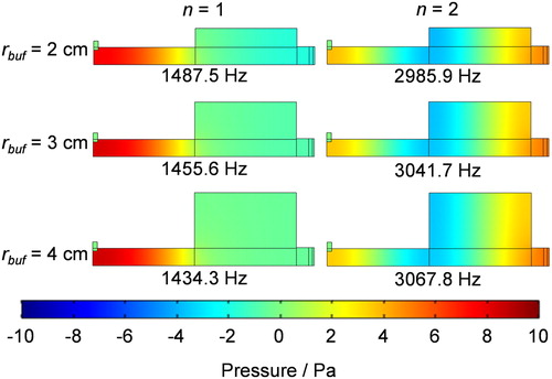
We used the model described in Section 3.1 to study the influence of both resonator (l_res, r_res) and buffer volume (l_buf, r_buf) dimensions on the acoustic properties of a single-resonator PA cell. In our model, we varied the dimensions of both buffer length (l_buf) and radius (r_buf), with l_buf varied from 0.1 l_res to 0.9 l_res in 0.1 l_res intervals and r_buf varied from 2.0 to 5.5 cm in 0.5 cm intervals. These studies were performed for the following combination sets of {l_res, r_res} to explore the influence of resonator dimensions on the acoustics: {11.0, 0.8}, {11.0, 0.9}, {11.0, 1.0}, {12.1, 1.0}, {13.2, 1.0}, where all dimensions are in centimeters. For l_res = 11.0 cm, r_res = 1.0 cm, and l_buf = 0.5 l_res, Figure 2 shows the model predictions of p_n($\overrightarrow{r}$) for the first two eigenmodes and how these eigenmode pressure distributions vary with r_buf. The eigenmode pressure at the microphone p_n(${\overrightarrow{r}}_{\mathrm{mic}}$) is large for the n = 1 mode and any excitation will be detected, while p_n(${\overrightarrow{r}}_M$) is weak for the n = 2 mode. Importantly, assuming a homogeneous α_abs throughout the PA cell and a laser beam with a $g\left(\overrightarrow{r}\right)$ that is invariant with laser beam propagation, the overlap integral $J_n=\int g\left(\overrightarrow{r}\right){\alpha }_{\mathrm{abs}}\left(\overrightarrow{r}\right)p_n\left(\overrightarrow{r}\right)dV$ that governs mode excitation (see Equations (10)(10) $$p\left({\overrightarrow{r}}_M,\omega \right)=\sum _n\frac{i\omega \left(\sigma -1\right)I_0}{\left({\omega }_n^2-{\omega }^2+i\frac{\omega {\omega }_n}{Q_n}\right)}\frac{\int g\left(\overrightarrow{r}\right){\alpha }_{\mathrm{abs}}\left(\overrightarrow{r}\right)p_n\left(\overrightarrow{r}\right)dV}{V}{p}_n\left({\overrightarrow{r}}_M\right)$$(10) and (11)(11) $$\left|p\left({\overrightarrow{r}}_M,\omega \right)\right|=\frac{\left(\sigma -1\right)I_0{J}_n{p}_n\left({\overrightarrow{r}}_M\right)}{V}\sqrt{\frac{Q_n^2/{\omega }_n^2}{1+Q_n^2{\left(\frac{{\omega }_n}{\omega }-\frac{\omega }{{\omega }_n}\right)}^2}}$$(11) ) is small for the n = 2 mode owing to similar contributions of positive and negative eigenmode pressure along the longitudinal (z) axis. Given the expected low excitation amplitude of the n = 2 mode and a weak p_n(${\overrightarrow{r}}_M$), detection of any n = 2 mode excitation is expected to be weak. Meanwhile, the n = 1 mode has mostly positive eigenmode pressure contributions to J_n along the longitudinal axis (particularly for large r_buf values) and this mode will be excited strongly.

Figure 2. The eigenmode pressure distributions p_n$\left(\overrightarrow{r}\right)$ for the first two eigenmodes of the single-resonator cell with l_res = 11.0 cm, r_res = 1.0 cm, l_buf = 5.5 cm and for variation of r_buf over the range 2–4 cm.

We performed simulations for the cases of acoustic excitation by either sample or window heating. Frequency-domain simulations were performed over the 1100–2100 Hz frequency range, with the absolute pressure response at the microphone location calculated for each frequency, giving $\left|p_{\mathrm{sig}}\left({\overrightarrow{r}}_M,\omega \right)\right|$ for sample heating and $\left|p_{\mathrm{bck}}\left({\overrightarrow{r}}_M,\omega \right)\right|$ for window heating. For some {l_buf, r_buf} combinations (notably, for l_buf ≥ 0.8 l_res), the frequency-dependent $\left|p\left({\overrightarrow{r}}_M,\omega \right)\right|$ response includes resonances from both the n = 1 and n = 2 modes within the 1100–2100 Hz frequency range (see Figure S1 in the SI). Both the n = 1 and n = 2 modes are longitudinal modes and their resonance frequencies decrease (acoustic wavelength increases) with increasing cell length. The decrease in eigenfrequency with increasing l_buf is particularly strong for the n = 2 mode because of the strong coupling of this mode to the buffer volume, while the n = 1 eigenmode pressure distribution is localized mostly to the resonator pipe (see Figure 2). Figure S1 in the SI confirms our aforementioned expectation that the signal due to sample excitation for the n = 2 mode is weaker than that of the n = 1 mode. To determine the resonance characteristic for each mode excitation, we used a non-linear least squares algorithm to fit a sum of two Lorentzian functions of the form: (16) $$\left|p\left({\overrightarrow{r}}_M,\omega \right)\right|=\sqrt{\frac{{p_1}^2}{1+{\left(2Q_1\frac{\left(\omega -{\omega }_1\right)}{{\omega }_1}\right)}^2}}+\sqrt{\frac{{p_2}^2}{1+{\left(2Q_2\frac{\left(\omega -{\omega }_2\right)}{{\omega }_2}\right)}^2}}$$(16) to the frequency-dependent $\left|p\left({\overrightarrow{r}}_M,\mathrm{ }\omega \right)\right|$ simulation data. We selected our best-fit coefficients {p₁, Q₁, ${\omega }_1$} to correspond to the lower-frequency resonance peak of interest (the n = 1 eigenmode), while the second set of coefficients {p₂, Q₂, ${\omega }_2$} either described a second, higher frequency eigenmode or served as a background correction when the simulation frequency range lacked a n = 2 mode excitation. This fitting procedure was performed for the simulations corresponding to both sample and window heating, giving the best-fit parameters $p_1^{\mathrm{sig}},$ $p_1^{\mathrm{bck}},$ Q₁, and ${\omega }_1$ (in addition to a second set of parameters corresponding to the n = 2 mode or a background correction) for each combination of the geometric parameters l_buf, r_buf, l_res, r_res described above. We then defined the SBR as: (17) $${\mathrm{SBR}}_{\mathrm{fit}}=\frac{p_1^{\mathrm{sig}}}{p_1^{\mathrm{bck}}}$$(17)

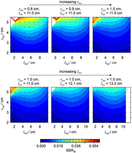
Figure 3 shows contour plots of the variation in SBR_fit with l_buf and r_buf, with different contour plots corresponding to different parameter combinations {l_res, r_res}. For completeness, the variations in Q₁ and f₁ can be found in SI Figure S2 for l_res = 11 cm, r_res = 1.0 cm. There were some combinations of l_buf and r_buf that either resulted in the resonant frequency for the n = 1 mode of interest not falling within the 1100–2100 Hz simulation region or the simulated pressure-frequency distributions were not described well by Equation (16)(16) $$\left|p\left({\overrightarrow{r}}_M,\omega \right)\right|=\sqrt{\frac{{p_1}^2}{1+{\left(2Q_1\frac{\left(\omega -{\omega }_1\right)}{{\omega }_1}\right)}^2}}+\sqrt{\frac{{p_2}^2}{1+{\left(2Q_2\frac{\left(\omega -{\omega }_2\right)}{{\omega }_2}\right)}^2}}$$(16) . Such parameter combinations can be identified by the blank regions on the SBR_fit contour plots. Figure 3 indicates an optimal value of l_buf = l_res/2 for maximizing the SBR_fit, while r_buf should be made as large as possible. We now study the trends in SBR_fit with l_buf and r_buf more closely.

Figure 3. Contour plots showing the variation in SBR_fit with changes in the buffer dimensions l_buf and r_buf, for multiple {l_res, r_res} combinations. The black points superimposed on the contour plots indicate the discrete value pairs {l_buf, r_buf} that were input to simulations.

For resonator dimensions l_res = 11.0 cm and r_res = 1.0 cm, Figure 4 shows profiles of $p_1^{\mathrm{sig}},$ $p_1^{\mathrm{bck}}$ and SBR_fit with variation in l_buf and r_buf. Figure 4 shows that $p_1^{\mathrm{sig}}$ is maximized for l_buf in the range 7.7–8.8 cm (0.7 l_res–0.8 l_res), while generally $p_1^{\mathrm{bck}}$ is minimized and SBR_fit is maximized at l_buf = 5.5 cm (0.5 l_res). We find, from inspecting the SBR_fit variations with l_buf for all {l_res, r_res} combinations, that SBR_fit is maximized at l_buf values close to l_res/2. Hence, setting l_buf = l_res/2 is a reliable design principle when designing buffer volumes for single-resonator PA cells. This is widely the case for the single-resonator cells used by many researchers (Bluvshtein et al. 2017; Lack et al. 2006, 2012; Bijnen, Reuss, and Harren 1996). We emphasize that setting l_buf = l_res/2 is a reliable design principle for single-resonator cells if the resonance of interest is longitudinal in nature; we show in the companion paper (Part 2) that cells with more sophisticated geometries sustain more complex pressure eigenmode fields and demonstrate different dependencies of SBR on the buffer dimensions.

Figure 4. The best-fit values for $p_1^{\mathrm{sig}},$ $p_1^{\mathrm{bck}},$ and SBR_fit with variation in l_buf. Model predictions are shown for different r_buf values. For these simulations, r_res = 1.0 cm and l_res = 11.0 cm. Lines are to guide the eye only.

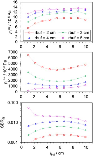
Figures 3 and 4 demonstrate that SBR_fit is significantly more sensitive to r_buf variation than similar magnitude changes in l_buf. For example, in simulations corresponding to l_res = 11.0 cm and r_res = 1.0 cm, 1 cm variations in l_buf resulted in an average SBR_fit change of ∼0.003, while the same magnitude variation in r_buf resulted in SBR_fit changing by ∼0.008. Similarly, Bijnen et al. reported a decrease in window background of ∼ 60 µPa W⁻¹ by increasing l_buf by 3 cm, but a decrease of almost 600 µPa W⁻¹ in window background upon increasing r_buf by 2 cm for their single-resonator cell (Bijnen, Reuss, and Harren 1996). This work thus supports the recommendation that the buffer radii should be kept as large as possible to maximize the SBR of single-resonator cells, recognizing that there are often physical restraints on how large photoacoustic devices can be made for many applications, including space available and the need to have low-volume cells for fast response times.

For r_buf = 5 cm, Figure 4 shows an increase in SBR_fit as l_buf decreases from 2.2 to 1.1 cm. This increase in SBR_fit is also indicated by the red areas in the SBR_fit contour plots (Figure 3) at small l_buf and large r_buf. These sudden increases in SBR_fit are caused by very effective suppression of the window background $p_1^{\mathrm{bck}}$ at specific buffer geometries, opposed to increased amplification of the sample signal $p_1^{\mathrm{sig}}.$ At the small l_buf and large r_buf for the range of geometries tested, the eigenmode pressure amplitude at the window locations, |p₁($\overrightarrow{r}$_win)|, tends to zero. For example, Figure 2 shows the strong reduction of |p_n($\overrightarrow{r}$_win)| for the n = 1 mode as r_buf increases from 2 to 4 cm. The optimal suppression of $p_1^{\mathrm{bck}}$ occurs when the dimensions of the buffer volumes are such that l_buf is similar to r_res while r_buf is close to l_res/2.

An alternative method to calculating SBR with changes in geometry is to use the eigenmode pressure distributions directly. Equation (11)(11) $$\left|p\left({\overrightarrow{r}}_M,\omega \right)\right|=\frac{\left(\sigma -1\right)I_0{J}_n{p}_n\left({\overrightarrow{r}}_M\right)}{V}\sqrt{\frac{Q_n^2/{\omega }_n^2}{1+Q_n^2{\left(\frac{{\omega }_n}{\omega }-\frac{\omega }{{\omega }_n}\right)}^2}}$$(11) shows that the microphone response $\left|p\left({\overrightarrow{r}}_M,\omega \right)\right|$ depends on several factors, including the spatial overlap integral J_n, with the resonant pressure amplitudes found by setting $\omega =\mathrm{ }{\omega }_n.$ From Equation (11)(11) $$\left|p\left({\overrightarrow{r}}_M,\omega \right)\right|=\frac{\left(\sigma -1\right)I_0{J}_n{p}_n\left({\overrightarrow{r}}_M\right)}{V}\sqrt{\frac{Q_n^2/{\omega }_n^2}{1+Q_n^2{\left(\frac{{\omega }_n}{\omega }-\frac{\omega }{{\omega }_n}\right)}^2}}$$(11) , we can define the modeled SBR as: (18) $${\mathrm{SBR}}_{\mathrm{model}}=\frac{\left|p_{\mathrm{sig}}\left({\overrightarrow{r}}_M,{\omega }_n\right)\right|}{\left|p_{\mathrm{bck}}\left({\overrightarrow{r}}_M,{\omega }_n\right)\right|}=\frac{\int g\left(\overrightarrow{r}\right){\alpha }_{\mathrm{abs},\mathrm{sample}}\left(\overrightarrow{r}\right)p_n\left(\overrightarrow{r}\right)dV}{\int g\left(\overrightarrow{r}\right){\alpha }_{\mathrm{abs},\mathrm{windows}}\left(\overrightarrow{r}\right)p_n\left(\overrightarrow{r}\right)dV}$$(18) with terms such as Q_n and ${\omega }_n$ from Equation (11)(11) $$\left|p\left({\overrightarrow{r}}_M,\omega \right)\right|=\frac{\left(\sigma -1\right)I_0{J}_n{p}_n\left({\overrightarrow{r}}_M\right)}{V}\sqrt{\frac{Q_n^2/{\omega }_n^2}{1+Q_n^2{\left(\frac{{\omega }_n}{\omega }-\frac{\omega }{{\omega }_n}\right)}^2}}$$(11) canceling out in the ratio $\left|p_{\mathrm{sig}}\left({\overrightarrow{r}}_M,{\omega }_n\right)\right|/\left|p_{\mathrm{bck}}\left({\overrightarrow{r}}_M,{\omega }_n\right)\right|,$ 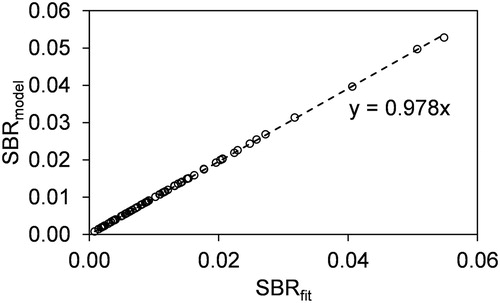except for the overlap integrals which are evaluated over different heating domains for sample and window heating. SBR_model corresponds to the ratio of overlap integrals evaluated directly from the FEM eigenmode pressure predictions, as opposed to SBR_fit that was calculated by fitting FEM pressure-frequency predictions to Equation (12)(12) $$\left|p\left({\overrightarrow{r}}_M,\omega \right)\right|=p_0\sqrt{\frac{1}{1+Q_n^2{\left(\frac{{\omega }_n}{\omega }-\frac{\omega }{{\omega }_n}\right)}^2}}$$(12) . To evaluate SBR_model, we calculated the overlap integrals over both sample and window heating domains using the same Gaussian distribution for $g\left(\overrightarrow{r}\right)$ as used in the frequency-domain simulations, i.e., a 0.5 mm beam waist that is invariant with beam propagation. For l_res = 11.0 cm and r_res = 1.0 cm, Figure 5 shows the correlation of SBR_model with SBR_fit for the combinations of l_buf and r_buf performed above. Comparing SBR_fit and SBR_model for the same values of l_buf and r_buf, the Pearson correlation coefficients were consistently 0.9999 for the different data sets corresponding to the five combinations of {l_res, r_res} and there is near-exact agreement between SBR_fit and SBR_model. Thus, calculation of SBR from knowledge of the eigenmode pressure distributions p_n($\overrightarrow{r}$) is a fast and accurate method for predicting cell performance. Importantly, we have shown that the p_n($\overrightarrow{r}$) govern cell performance when the background is dominated by laser-window interactions.

Figure 5. For l_res = 11.0 cm and r_res = 1.0 cm, SBR_model plotted against the SBR_fit for corresponding l_buf, r_buf values. We calculated SBR_model using Equation (18)(18) $${\mathrm{SBR}}_{\mathrm{model}}=\frac{\left|p_{\mathrm{sig}}\left({\overrightarrow{r}}_M,{\omega }_n\right)\right|}{\left|p_{\mathrm{bck}}\left({\overrightarrow{r}}_M,{\omega }_n\right)\right|}=\frac{\int g\left(\overrightarrow{r}\right){\alpha }_{\mathrm{abs},\mathrm{sample}}\left(\overrightarrow{r}\right)p_n\left(\overrightarrow{r}\right)dV}{\int g\left(\overrightarrow{r}\right){\alpha }_{\mathrm{abs},\mathrm{windows}}\left(\overrightarrow{r}\right)p_n\left(\overrightarrow{r}\right)dV}$$(18) and used overlap integrals J_n calculated from FEM simulations of p_n$\left(\overrightarrow{r}\right).$ The Pearson correlation coefficient between SBR_model and SBR_fit is 0.9999.

4.1.2. Comparison of FEM predictions with measurements

We now compare model predictions of PA cell performance with measurements. Section 3.2. described our measurement procedure. The geometric parameters that describe the resonator pipe of our measurement cell are very slightly different from those used in the model simulations in the previous section; l_res was measured as 11.2 cm and r_res as 1.1 cm. Thus, for the work in this section, we re-ran our FEM model using the geometric parameters that reflect our measurement cell. As described in Section 3.2, we measured cell performance for various buffer volume inserts, with r_buf taking values of 2, 3, 4, and 5 cm.

Figure 6a compares the measured frequency-domain cell response using speaker excitation with the predicted $\left|p_{\mathrm{sig}}\left({\overrightarrow{r}}_M,\omega \right)\right|.$ Using a speaker to excite the cell facilitates the fast measurement of the eigenmode distribution by providing an excitation source at all frequencies of interest. Conversely, using the laser source to heat an ozone sample would take more time; the laser modulation frequency would need to be changed manually in 1 Hz intervals over the frequency range 1300–1500 Hz and the IA recorded for several seconds at each frequency. The measured distributions are predicted well by our FEM model, with the measured and modeled resonance frequencies in agreement to within 0.25%. The measured resonance frequencies are ∼3.5 Hz lower compared to FEM predictions, most likely caused by discrepancies in the air temperature. The speed of sound in air is sensitive to small changes in temperature. Our measurement cell was not temperature stabilized and a decrease in temperature from 20 to 19 °C corresponds to a decrease in the speed of sound by 0.6 m s⁻¹ and a ∼2.5 Hz decrease in resonance frequency for the n = 1 eigenmode. Moreover, the 0.1 mm measurement uncertainty in l_res corresponds to ∼1.4 Hz error in the predicted resonance frequency. Therefore, the ∼3.5 Hz discrepancy between predicted and measured resonance frequencies is within experimental error associated with uncertainties in air temperature and resonator pipe length. Figure 6a also shows that the measured and predicted mode widths are broadly in excellent agreement, except for the smallest r_buf value. For r_buf = 2 cm, Q is measured as 66.8 and is significantly reduced compared to the predicted value of 130.2. Figure 2 shows that the n = 1 eigenmode pressure amplitude increases within the buffer and window volumes as r_buf decreases. Therefore, we associate the reduced Q for r_buf = 2 cm with increased contributions to acoustic damping from the buffer and window volumes. Indeed, while the resonator pipe had a polished surface, the buffer and window volume surfaces were not polished, with our FEM model neglecting the impact of surface roughness on damping. Moreover, the impedance of the sample inlet/outlet ports within the buffer volumes is neglected in our model and will contribute more to acoustic damping at small buffer radii. Figure 6a also shows that there is good agreement between model and measurement for the relative mode amplitude with variation in r_buf, except for r_buf = 2 cm. This poor agreement at small r_buf is associated with the significant acoustic damping described above.

Figure 6. (a) Comparison of measured frequency-dependent variations in IA (points) with FEM predictions of $\left|p_{\mathrm{sig}}\left({\overrightarrow{r}}_M,\omega \right)\right|$ (lines). Data are shown for r_buf values of 2, 3, 4, and 5 cm. (b) Comparison of measured IA_sig,cor and predicted $\left|p_{\mathrm{sig}}\left({\overrightarrow{r}}_M,{\omega }_n\right)\right|$ values. (b) Comparison of measured IA_sig,bck and predicted $\left|p_{\mathrm{bck}}\left({\overrightarrow{r}}_M,{\omega }_n\right)\right|$ values. (d) Comparison of measured and predicted SBR values. Error bars represent one standard error in the measured quantities. The geometric parameters describing our measurement cell and those used in our FEM calculations are: l_res = 11.2 cm, r_res = 1.1 cm, l_buf = 5.5 cm, l_win = 1.0 cm, r_win = 1.0 cm. The dashed lines are to guide the eye only.

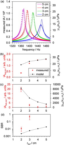
We also measured IA_sig and IA_bck using the procedure described in Section 3.2. The measured IA values were normalized for small changes in RMS laser power, while IA_sig was also normalized to an effective sample absorption level of 5 Mm⁻¹, giving IA_sig,corr and IA_bck,corr. The measured SBR is then defined as the ratio IA_sig,corr/IA_bck,corr. Figure 6b compares the measured IA_sig,cor and predicted $\left|p_{\mathrm{sig}}\left({\overrightarrow{r}}_M,{\omega }_n\right)\right|,$ Figure 6c compares the measured IA_bck,cor and predicted $\left|p_{\mathrm{bck}}\left({\overrightarrow{r}}_M,{\omega }_n\right)\right|,$ and Figure 6d compares the measured and predicted SBR. The general trends in IA_sig,cor, IA_bck,cor, and SBR with change in r_buf are predicted well by our model. The trends in IA_sig,cor and $\left|p_{\mathrm{sig}}\left({\overrightarrow{r}}_M,{\omega }_n\right)\right|$ with r_buf disagree for r_buf = 2 cm, with the measured IA_sig,cor lower than expected. This discrepancy is partly attributed to the low Q measured for this cell; correcting for the low Q of the cell would give an IA_sig,corr value of 0.73 that is still low compared to our model expectation. Additional discrepancies between IA_sig,corr and $\left|p_{\mathrm{sig}}\left({\overrightarrow{r}}_M,{\omega }_n\right)\right|$ are likely attributed to the fact that the role of the sample inlet and outlet ports are neglected, which will become increasingly important at small r_buf values. Discrepancies between IA_bck,cor and $\left|p_{\mathrm{bck}}\left({\overrightarrow{r}}_M,{\omega }_n\right)\right|$ are difficult to assess as there are large uncertainties in the measured IA_bck,cor for r_buf = 4, 5 cm. For these larger buffer radii, SI Figure S3 shows that the IA_bck for laser-window interactions were indistinguishable from the noise in the IA with the laser off, with the latter measurement associated with electronic and flow noise. The large uncertainty in the measured IA_bck prevented meaningful calculations of SBR for r_buf = 4, 5 cm and, therefore, Figure 6d omits SBR values for these largest r_buf values. Our measured SBR values are 10–95 times higher than model predictions. This discrepancy between model and predicted SBR is likely caused by our lack of consideration of the effect of the inlet and outlet geometries on the acoustics, and how laser-window interactions are represented in our model, leading to an overestimation of $p_1^{\mathrm{bck}}.$ For example, our model places a window heating volume within the PA cell, while the measurement cell has windows fixed to the external aluminum cell surface and heat deposited in the windows are removed by air both inside and external to the cell. Moreover, heat will be removed by efficient conduction to the solid surfaces that a window is in contact with. Representing this conduction process in addition to modeling the thermo-viscous acoustics of the PA cell would increase the model complexity significantly and was not attempted. Regarding the lack of consideration for the effect of the inlet and outlet geometries on the acoustic behavior of the PA cell, it would have been desirable to include these geometries in our model calculations. However, addition of these geometries increases the dimensionality of our model (from 2D axisymmetric to 3D) and reduces the model symmetry such that this simulation is too expensive for the computational power we have available if we maintain our mesh parameter selection at a fine enough resolution to adequately resolve both bulk and surface acoustic phenomena. While the absolute value of the SBR is not predicted correctly due to uncertainties in how to represent the window heat transfer processes, trends in the measured IA_sig,cor, IA_bck,cor and SBR with variation in cell dimensions can be determined reliably.

The work in this section has demonstrated that FEM can predict accurately PA cell resonance frequencies and mode distributions in the frequency domain, in addition to trends in IA_sig,cor, IA_bck,corr, and SBR with variation in cell dimensions. We show further comparisons of model predictions and measurements in Section 4.3.1. We now explore various strategies to improve the performance of our single-resonator cell, including the use of multiple buffer volumes or the addition of TACs.

4.2. The influence of multiple buffer volumes on PA cell performance

Brand et al. (1995) used multiple buffer volumes to suppress the detection of various sources of background and noise. It is useful to consider whether the addition of extra buffer volumes to our single-resonator cell leads to improvements in SBR. This section studies the impact of two buffer volumes in series capping each end of our single-resonator cell on acoustic behavior. Figure 7a shows the geometry of our cell used in FEM simulations, consisting of a cylindrical resonator with l_res = 11.0 cm, r_res = 1.0 cm capped by two cylindrical buffer volumes in series at each resonator end. These buffer volumes have matching values for l_buf and r_buf. A separating tube between the two buffer volumes has a length l_sep and radius r_sep. In all the simulations performed here, r_sep = r_res. We present the results of two separate studies. First, we study the cell acoustic performance with variation in l_buf and r_buf, while keeping the separation volume constant with l_sep = l_res/8 (1.4 cm). Second, we study the cell acoustic performance with variation in l_buf and l_sep, while keeping the buffer radius constant at r_buf = 1.7 cm.

Figure 7. (a) The geometry of the double-buffer single-resonator PA cell, with a rotational axis of symmetry (red dashed line) and a reflection symmetry plane (blue dotted line). (b) and (c) The pressure eigenmode distributions for the n = 1 and n = 2 modes, respectively, for l_buf = 5.5 cm and r_buf = 1.7 cm. Other geometric parameters: l_res = 11.0 cm, r_res = 1.0 cm, l_sep = 1.38 cm, r_sep = 1 cm, l_win = 1.0 cm, r_win = 1 cm.

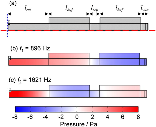
Before performing these two studies, an eigenmode search was performed over the frequency range 0–2000 Hz for r_buf =1.7 cm, l_buf = 0.5 l_res, l_sep = l_res/8. Figures 7b and c show the p_n($\overrightarrow{r}$) for the two eigenfrequencies within the 0–2000 Hz search range. The n = 1 eigenfrequency is below 1000 Hz and will therefore be more susceptible to detection of ambient noise in measurements. Thus, the simulations presented here investigate excitation and subsequent detection of the n = 2 mode.

4.2.1. Varying l_buf and r_buf

We varied l_buf from 0.2 l_res to 0.8 l_res in 0.1 l_res intervals and r_buf from 2 to 5 cm in 0.5 cm intervals. Figure 8a shows the predicted SBR_fit with variation in both l_buf and r_buf, showing similar trends as seen for the single buffer case (see Figure 3). Figure 9 compares p^sig, p^bck, and SBR_fit for the double-buffer PA cell with the values retrieved for the single-buffer case. Values are compared for the same parameter combinations {l_buf, r_buf}. The p^sig are 9% lower on average for the double-buffer case, while p^bck from window heating are 80% lower. For all combinations of l_buf and r_buf, the average SBR is 670% higher for the double-buffer cell. However, the magnitude of the increase in SBR by including double buffers depends strongly on the buffer dimensions. Generally, the introduction of a second buffer volume suppresses the background and significantly improves the SBR.

Figure 8. For a single–resonator PA cell with double-buffer volumes capping each resonator end, (a) SBR_fit with variation in l_buf and r_buf for l_sep = 1.38 cm; (b) SBR_fit with variation in l_buf and l_sep for r_buf = 1.7 cm. For all simulations, l_res = 11.0 cm, r_res = 1.0 cm, r_sep = 1 cm.

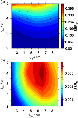
Figure 9. (a–c) Comparison of p^sig, p^bck, and SBR_fit for a single-resonator PA cell with either a single or double buffer volume capping each resonator end (black circles). Comparisons are made between buffer volumes with the same values of l_buf, r_buf. In the double-buffer case, the buffers are separated by a tube with l_sep = 1.38 cm and r_sep = 1.0 cm. The dashed red line represents a 1:1 line for comparison purposes. (d) The relative SBR difference (SBR_{double_bufer} – SBR_{single_buffer})/SBR_{single_buffer} as a percentage with varying r_buf. Other parameters: l_res = 11.0 cm, r_res = 1.0 cm.

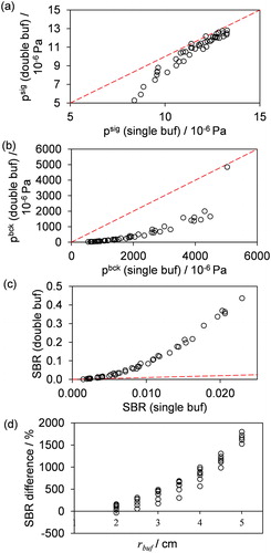
Figure 9d shows the percentage difference in SBR between the double and single buffer cases, showing a strong trend in SBR difference with r_buf. Meanwhile, we find little dependency of this percentage difference on l_buf. The SBR is improved by including a second buffer volume only when r_buf > 2 cm; including a second buffer volume can be detrimental to the SBR if r_buf < 2 cm. We emphasize that other geometric parameters, such as the resonator geometry, will determine whether using double buffer volumes is beneficial or detrimental to cell performance. Furthermore, only window heating contributions to the background are considered here; as p^bck is suppressed upon inclusion of double-buffer volumes with r_buf > 2 cm, the predicted improvements in SBR may not be realized as other background and noise sources begin to dominate. We now explore further the observed detrimental impact on SBR of using double-buffers for the case r_buf < 2 cm.

4.2.2. Varying l_buf and l_sep

The simulations above arbitrarily used l_sep = l_res/8 = 1.4 cm. We now investigate varying the lengths l_buf and l_sep on the detected pressures and SBR. We varied l_buf over the range 0.2 l_res–0.8 l_res in 0.1 l_res intervals and l_sep over the range 1–5 cm in 1 cm intervals, while r_buf was set to 1.7 cm. We chose this r_buf value from considering the physical limitations on the PAS cell width for our own particular application, while this value is less than the r_buf = 2 cm threshold for achieving an improvement in the SBR with the addition of double-buffer volumes for the cell dimensions considered in the last section. Figure 8b shows a contour plot of SBR_fit with variation in l_buf and l_sep, clearly indicating a SBR maximum at l_buf = 0.6 l_res and l_sep = 4 cm. At this maximum, SBR_fit = 0.004 and is the same value as for a single-buffer case with l_buf = 0.6 l_res. Again, the addition of a second buffer volume is not beneficial for r_buf < 2 cm. This emphasizes the importance of solving the acoustics for a given geometry to determine the PA cell performance and not forming general rules for cell geometry.

4.3. The influence of TACs on PA cell performance

For the single-resonator cell, we have explored the influence of both buffer volume size and multiple buffer volumes on detection of window heating and the SBR. Another strategy found in the literature for suppressing the window background is the addition of tunable TACs (Bijnen, Reuss, and Harren 1996; Miklós and Lörincz 1989). A TAC is a cylindrical pipe of length l_TAC and radius r_TAC that extends from a PA cell window volume, with one end open to the window volume and the other end closed. We note that TACs are often located after both the window and the sample inlet/outlet. Therefore, TACs are tasked with suppressing background contributions from both laser-window interactions and sample flow noise. However, as we have already noted, the flow noise for the 1.0 L min⁻¹ flow rates used were insignificant in comparison to the dominant window noise. Bijnen, Reuss, and Harren (1996) studied the influence of TACs on |p_bck$\left({\overrightarrow{r}}_M,\mathrm{ }{\omega }_n\right)$| for a single-resonator cell through a combination of experiment and predictions from transmission line theory. The authors reported excellent agreement between measurements and model predictions, with optimal window background suppression occurring for l_TAC = l_res/2. However, this result pertains to the authors’ gas photoacoustic cell that has a very narrow resonator pipe (r_res = 3 mm) and buffer volumes of large radius compared to the resonator radius (r_buf = 20 mm). Moreover, the authors did not report variations in $\left|p_{\mathrm{sig}}\left({\overrightarrow{r}}_M,{\omega }_n\right)\right|$ or the SBR, preventing a full assessment of the impact of TACs on instrument performance. We used FEM to simulate the eigenmodes and frequency-dependent pressures $\left|p_{\mathrm{sig}}\left({\overrightarrow{r}}_M,{\omega }_n\right)\right|$ and $\left|p_{\mathrm{bck}}\left({\overrightarrow{r}}_M,{\omega }_n\right)\right|$ for the geometries reported by Bijnen, Reuss, and Harren (1996), verifying that FEM predicts the same trends in $\left|p_{\mathrm{bck}}\left({\overrightarrow{r}}_M,{\omega }_n\right)\right|$ with varying l_TAC as the literature measurements. We then used FEM to predict the impact of TACs on acoustic performance for the aerosol cell studied in previous sections.

4.3.1. Reproducing literature measurements for PA cells with TACs

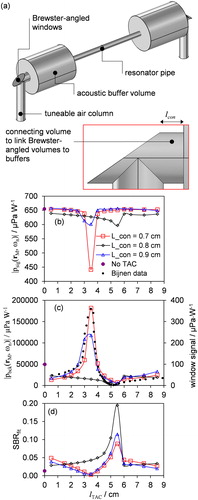
Figure 10a shows the geometry used in our simulations to describe the cell used by Bijnen, Reuss, and Harren (1996). The cylindrical resonator had dimensions l_res = 100 mm, r_res = 3 mm and buffer volumes had dimensions l_buf = 50 mm, r_buf = 20 mm. The window volumes consisted of a cylindrical volume (l_con, r_con) connecting a Brewster-angled volume to the buffers. Bijnen, Reuss, and Harren (1996) did not report the Brewster angle used in their setup, and we used θ_B = 67.4° based on the authors using ZnSe windows and a CO₂ IR laser source. We investigated the influence of small changes of ∼ 2–3 degrees to θ_B. Moreover, the authors did not specify the value of l_con, and thus we tried values in the range 7–10 mm. The cross-section radius of the Brewster volumes and r_con were both 5 mm. Consistent with the measurements by Bijnen, Reuss, and Harren (1996), the length of one column was fixed at l_TAC = l_res/2 = 50 mm while the length of the second TAC was varied from 5 to 85 mm.

Figure 10. (a) The cell geometry used by Bijnen, Reuss, and Harren (1996). The predicted variation in (b) |p_sig(${\overrightarrow{r}}_M,{\omega }_n$)|, (c) |p_bck(${\overrightarrow{r}}_M,{\omega }_n$)|, and (d) SBR_fit with l_TAC for the Bijnen cell. The length of only one TAC was varied, while the length of the other was set to 5 cm. We report predictions using l_con values of 7, 8, and 9 mm, in addition to the predictions for a cell with no TACs with l_con = 7 mm. In (c), we compare our predictions of |p_bck(${\overrightarrow{r}}_M,{\omega }_n$)| with measurements from Bijnen, Reuss, and Harren (1996) for window heating excitation of the PA cell. Lines are to guide the eye only.

For these simulations, the addition of TACs and Brewster-angled windows to our single-resonator model broke the rotational symmetry and thus we used a 3D model. The reduced model symmetry results in a high number of mesh elements, leading to longer computation times. Consequently, we used a lower resolution mesh for our 3D model simulations compared to that used in our 2D axisymmetric models, with the parameters used to calculate this mesh described in Section SI.1.2. of the SI. We performed frequency-domain simulations for window heating using the same heating model described earlier albeit with α_abs = 0.2 m⁻¹, i.e., the value for ZnSe windows (Bijnen, Reuss, and Harren 1996), and cylindrical window heating volumes were oriented at the Brewster angle with respect to the laser beam propagation direction.

Figure 10c shows the FEM predictions of |p_bck$\left({\overrightarrow{r}}_M,{\omega }_n\right)$| for cases of l_con = 7, 8, 9 mm and θ_B = 67.4°. Also shown is the response reported by Bijnen, Reuss, and Harren (1996), which can be interpreted as either the authors transmission line theory prediction or the values from experiment which used a rear window that was blackened to increase absorption levels. The authors scaled their measured |p_bck$\left({\overrightarrow{r}}_M,{\omega }_n\right)$| values to their theoretical calculations. Therefore, we have scaled the vertical axis on which the authors’ data are plotted such that the maximum for the Bijnen data in Figure 10c agrees with the maximum of our model prediction for l_con = 7 mm. The simulation using l_con = 7 mm agrees well with the Bijnen data, correctly predicting a maximum in |p_bck$\left({\overrightarrow{r}}_M,{\omega }_n\right)$| located at l_TAC = 3.5 cm, while |p_bck$\left({\overrightarrow{r}}_M,{\omega }_n\right)$| is minimized at l_TAC values close to l_res/2 = 50 mm. We found that changes to θ_B less than 3° had only a minor impact on |p_bck$\left({\overrightarrow{r}}_M,{\omega }_n\right)$|. The small discrepancies between our best-fit prediction and the data of Bijnen et al. are expected to arise from the exact values of both l_con and θ_B being unknown. However, the agreement between our model prediction using l_con = 7 mm and the measured Bijnen data again emphasizes that our FEM model predicts PA cell acoustic properties reliably.

We repeated the above FEM simulations for acoustic excitation by sample heating with α_abs = 5 Mm⁻¹. Figures 10b and d show predictions for |p_sig(${\overrightarrow{r}}_M,{\omega }_n$)| and SBR, respectively, with variation in l_TAC. For all l_con values, the SBR is maximized when l_TAC = 5.5 cm. It is important to compare our FEM predictions for the PA cells including TACs with that for a cell with no TACs. Therefore, Figures 10b–d also show the predicted signal, background and SBR for the cell without TACs and with l_con = 7 mm. It is clear that the inclusion of TACs improves the SBR markedly. For l_con = 7 mm, the SBR improves from 0.014 for the no-TAC case to 0.088 when TACs are included with l_TAC = 5.5 cm, an improvement in SBR by a factor of 6.3.

We have now established that the incorporation of TACs into PA cell geometries can greatly improve PA cell performance. However, we have assessed the impact of TACs for a single-resonator cell with a geometry that is markedly different to an aerosol cell. In particular, the ratio r_buf/r_res for the Bijnen cell is large. Thus, we now assess the impact of TACs on acoustic performance for a PA cell with a large r_res suitable for aerosol detection.

4.3.2. The influence of TACs on the performance of an aerosol PA cell

We used FEM to study the influence of TACs on acoustic performance for our single-resonator cell suitable for aerosol detection. Our model included flat windows, opposed to Brewster-angled windows, so that our predictions can be compared to those presented in previous sections. The lengths and radii (l, r) for the cylindrical sections of the cell were (11.0, 1.0) for the resonator, (5.5, 1.7) for the buffer volumes and (1.0, 1.0) for the window volumes, where all dimensions are in centimeters. A TAC was connected to the center of each window volume. We varied both l_TAC and r_TAC for both TACs simultaneously, with the dimensions of both columns assigned the same values of l_TAC and r_TAC.

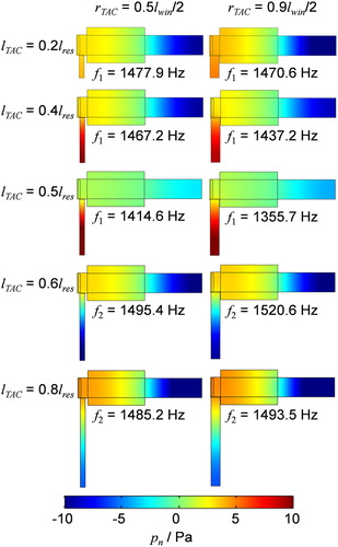
We performed an eigenmode analysis to inspect the eigenmode pressure distributions p_n in the frequency range 1–2000 Hz. This eigenmode study was performed for variation in l_TAC from 0.2 l_res to 0.8 l_res, and r_TAC from 0.05 l_win to 0.45 l_win. The n = 1 eigenmode became undetectable at the microphone location for l_TAC values greater than l_res/2, with p₁$\left({\overrightarrow{r}}_M,{\omega }_1\right)$ ≈ 0. When the n = 1 mode became undetectable, the n = 2 eigenmode became the mode of interest as this mode had a detectable pressure p₂$\left({\overrightarrow{r}}_M,{\omega }_2\right)$ at the microphone location. Figure 11 shows the predicted eigenmode pressure distributions for l_TAC values in the range 0.2 l_res–0.8 l_res and r_TAC = 0.25 l_win, 0.45 l_win, labeling the eigenmode order and its associated eigenfrequency. The p_n$\left(\overrightarrow{r}\right)$ distribution changes markedly as l_TAC approaches a value of l_res/2. At this TAC length, the eigenmode pressure amplitude approaches zero at the window boundaries (indicating that laser-window interaction sources will couple less efficiently into the eigenmode), while the p_n$\left(\overrightarrow{r}\right)$ magnitude over the full path length of the laser beam through the cell is reduced (indicating that sample heating sources will couple less efficiently into the eigenmode).

Figure 11. For a single-resonator aerosol PA cell with TACs, FEM predictions of p_n($\overrightarrow{\mathrm{r}}$) for the detectable eigenmode in the eigenfrequency range 1–2000 Hz, with variation in l_TAC and r_TAC. The values for other cell dimensions are provided in the main text.

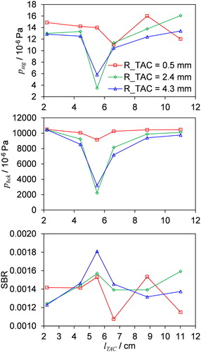
We used FEM to simulate the microphone responses $\left|p_{\mathrm{sig}}\left({\overrightarrow{r}}_M,\mathrm{ }\omega \right)\right|$ and $\left|p_{\mathrm{bck}}\left({\overrightarrow{r}}_M,\mathrm{ }\omega \right)\right|$ using α_abs,sample = 5 Mm⁻¹ and α_abs,win = 0.1653 m⁻¹, respectively. These simulations were performed over the frequency range 1300–1600 Hz, for l_TAC varying over the range 0.2 l_res–1.0 l_res in 0.2 l_res steps and for r_TAC values of 0.05 l_win, 0.25 l_win and 0.45 l_win. The frequency-dependent data were fit to a single Lorentzian to determine Q, f and the amplitudes $p_n^{\mathrm{sig}}$ or $p_n^{\mathrm{bck}}$ depending on the heating source. Figure 12 shows the variation in $p_n^{\mathrm{sig}},$ $p_n^{\mathrm{bck}},$ and SBR_fit with l_TAC for the different values of r_TAC used. For completeness, we show the variations in Q and f in Figure S4 of the SI. The $p_n^{\mathrm{bck}}$ are significantly reduced for l_TAC = l_res/2 = 5.5 cm for all r_TAC values. However, $p_{\mathrm{sig}}$ is also significantly reduced at l_TAC values close to l_res/2 owing to the reduction in the eigenmode pressure over the entire laser path length (Figure 11), reducing both the overlap integral J_n for sample heating and the eigenmode pressure at the microphone location. The SBR, i.e., the most important metric for assessing cell performance, is not necessarily optimized at l_TAC = l_res/2. We find that SBR_fit does not vary smoothly with l_TAC. Only for the largest value of r_TAC = 0.45 l_win is there a clear SBR_fit maximum at l_TAC = l_res/2, with SBR_fit = 0.0018 for this optimized TAC case. However, it is important to place any improvement in SBR upon addition of TACs in context with the no-TAC cell. Our simulations predict SBR = 0.0015 for the no-TAC case and we expect only a small improvement of 0.0003 (20%) in SBR upon addition of optimal TACs. Furthermore, Figure 12 shows that the SBR_fit is highly sensitive to small (millimetre) changes to TAC dimensions and, therefore, it could be difficult to achieve even a small SBR improvement for experimental cells where manufacturing precision may be limited.

Figure 12. For a single-resonator aerosol PA cell with tunable air columns, the variation in p^sig, p^bck, and SBR_fit with l_TAC, with different data series corresponding to different r_TAC values. Lines are to guide the eye only.

Ultimately, the impact of TACs on PA cell performance depends strongly on the dimensions of other cell domains, such as the resonator pipe, buffer and window volumes. In particular, we find that TACs are highly beneficial for improving SBR in the Bijnen trace gas PA cell with r_buf/r_res = 6.7, while TACs have little influence on SBR for the aerosol cell studied in this section with r_buf/r_res = 1.8. Researchers should consider using TACs in their PA cells but must assess the influence of TACs on SBR for their specific cell geometry.

5. Summary

We have developed a FEM model to assess the acoustic properties of multipass PA cells suitable for measuring aerosol absorption coefficients. This model is useful for informing decisions on PA cell geometry for optimal sensitivity. By comparing our model predictions with a combination of our own measurements and those in the literature, we have shown that our model predicts accurately the resonance frequencies and acoustic eigenmode distributions for PA cells, in addition to predicting reliably the trends in microphone responses and SBR with variation in cell dimensions. We emphasize that quantitative estimates of SBR are not possible unless the exact mechanism of laser-window interactions and all subsequent energy transfer pathways are known.

We have studied the optimization of various PA cell dimensions and the impact on SBR of including double-buffer volumes or TACs. In particular, the SBR is consistently maximized for a single-resonator cell when l_buf = l_res/2 and for large r_buf. These criteria may not hold true (as we demonstrate in a companion paper) for cell geometries that differ significantly from the single-resonator cell structure considered in this article. We have demonstrated that the inclusion of multiple buffer volumes can significantly increase the SBR only if certain criteria are met for other cell dimensions. Specifically, for a cell with a resonator length and radius of 11.0 cm and 1.0 cm, respectively, the SBR is improved by using double-buffers only when the radii of the buffer volumes are >2 cm. Moreover, while previous researchers have advocated the inclusion of TACs for reducing the detection of laser-window interactions, we find that including TACs has little impact on the SBR for cells with resonator dimensions commonly found in aerosol PAS instruments. We recommend strongly that researchers perform optimization studies when designing a PA cell for their own applications rather than relying on general design principles.

Finally, this article forms the model basis for a companion paper (Cotterell et al. 2019b) that assesses the acoustic properties and optimization of a common two-resonator cell that has been adopted by several international research groups for laboratory and airborne field studies. This companion article provides further measurements validating the reliability of our FEM model in predicting acoustic properties.

Disclosure statement

No potential conflict of interest was reported by the authors.

Data availability

For data related to this article, please contact Michael I. Cotterell ([email protected]) or Justin M. Langridge ([email protected]).

Additional information

Funding

This work was supported through a Royal Society of Chemistry/Analytical Chemistry Trust Fund Tom West Fellowship awarded to Michael I. Cotterell. Jim M. Haywood and Michael I. Cotterell thank the Natural Environment Research Council for support through the CLARIFY-2017 grant (NE/L013797/1). The Met Office funded experimental measurements. The Research Council on Norway provided further instrument support via the projects AC/BC (240372) and NetBC (244141).

References

- Anderson, T. L., S. J. Masonis, D. S. Covert, N. C. Ahlquist, S. G. Howell, A. D. Clarke, C. S. McNaughton. 2003. Variability of aerosol optical properties derived from in situ aircraft measurements during ACE-Asia. J. Geophys. Res. 108 (D23):ACE 15-1–ACE 15-19. doi: 10.1029/2002JD003247.
- Arnott, W. P., H. Moosmüller, C. F. Rogers, T. Jin, and R. Bruch. 1999. Photoacoustic spectrometer for measuring light absorption by aerosol: Instrument description. Atmos. Environ. 33 (17):2845–2852. doi: 10.1016/S1352-2310(98)00361-6.
- Arnott, W. P., J. W. Walker, H. Moosmüller, R. A. Elleman, H. H. Jonsson, G. Buzorius, W. C. Conant, R. C. Flagan, and J. H. Seinfeld. 2006. Photoacoustic insight for aerosol light absorption aloft from meteorological aircraft and comparison with particle soot absorption photometer measurements: DOE Southern Great Plains climate research facility and the coastal stratocumulus imposed perturbat. J. Geophys. Res. 111 (D5):D05S02. doi: 10.1029/2005JD005964.
- Baumann, B., B. Kost, H. Groninga, and M. Wolff. 2006. Eigenmode analysis of photoacoustic sensors via finite element method. Rev. Sci. Instrum. 77 (4):044901. doi: 10.1063/1.2186808.
- Baumann, B., M. Wolff, B. Kost, and H. Groninga. 2007. Finite element calculation of photoacoustic signals. Appl. Opt. 46 (7):1120–1125. doi: 10.1364/AO.46.001120.
- Bijnen, F. G. C., J. Reuss, and F. J. M. Harren. 1996. Geometrical optimization of a longitudinal resonant photoacoustic cell for sensitive and fast trace gas detection. Rev. Sci. Instrum. 67 (8):2914–2923. doi: 10.1063/1.1147072.
- Bluvshtein, N., J. M. Flores, Q. He, E. Segre, L. Segev, N. Hong, A. Donohue, J. N. Hilfiker, and Y. Rudich. 2017. Calibration of a multi-pass photoacoustic spectrometer cell using light-absorbing aerosols. Atmos. Meas. Tech. 10 (3):1203–1213. doi: 10.5194/amt-10-1203-2017.
- Bond, T. C., T. L. Anderson, and D. Campbell. 1999. Calibration and intercomparison of Filter-Based measurements of visible light absorption by aerosols. Aerosol Sci. Technol. 30 (6):582–600. doi: 10.1080/027868299304435.
- Brand, C., A. Winkler, P. Hess, A. Miklós, Z. Bozóki, and J. Sneider. 1995. Pulsed-laser excitation of acoustic modes in open high-Q photoacoustic resonators for trace gas monitoring: results for C(2)H(4). Appl. Opt. 34 (18):3257–3266. doi: 10.1364/AO.34.003257.
- Cappa, C. D., D. A. Lack, J. B. Burkholder, and A. R. Ravishankara. 2008. Bias in Filter-Based aerosol light absorption measurements due to organic aerosol loading: Evidence from laboratory measurements. Aerosol Sci. Technol. 42 (12):1022–1032. doi: 10.1080/02786820802389285.
- COMSOL User’s Guide. 2016. Acoustics Module User’s Guide COMSOL Multiphysics 5.2a. COMSOL.
- Cotterell, M. I., A. J. Orr-Ewing, K. Szpek, J. M. Haywood, and J. M. Langridge. 2019a. The impact of bath gas composition on the calibration of photoacoustic spectrometers with ozone at discrete visible wavelengths spanning the Chappuis band. Atmos. Meas. Tech. 12 (4):2371–2385. doi: 10.5194/amt-12-2371-2019.
- Cotterell, M. I., T. C. Preston, A. J. Orr-Ewing, and J. P. Reid. 2016. Assessing the accuracy of complex refractive index retrievals from single aerosol particle cavity ring-down spectroscopy. Aerosol Sci. Technol. 50 (10):1077–1095. doi: 10.1080/02786826.2016.1219691.
- Cotterell, M. I., G. P. Ward, A. P. Hibbins, J. M. Haywood, A. Wilson, and J. M. Langridge. 2019b. Optimizing the performance of aerosol photoacoustic cells using a finite element model. Part 2: Application to a two-resonator cell. Aerosol Sci. Technol. doi: 10.1080/02786826.2019.1648749.
- Cotterell, M. I., R. E. Willoughby, B. R. Bzdek, A. J. Orr-Ewing, and J. P. Reid. 2017. A complete parameterisation of the relative humidity and wavelength dependence of the refractive index of hygroscopic inorganic aerosol particles. Atmos. Chem. Phys. 17 (16):9837–9851. doi: 10.5194/acp-17-9837-2017.
- Cremer, J. W., P. A. Covert, E. A. Parmentier, and R. Signorell. 2017. Direct measurement of photoacoustic signal sensitivity to aerosol particle size. J. Phys. Chem. Lett. 8 (14):3398–3403. doi: 10.1021/acs.jpclett.7b01288.
- Cremer, J. W., K. M. Thaler, C. Haisch, and R. Signorell. 2016. Photoacoustics of single laser-trapped nanodroplets for the direct observation of nanofocusing in aerosol photokinetics. Nat. Commun. 7 (1):10941.
- Davies, N. W., M. I. Cotterell, C. Fox, K. Szpek, J. M. Haywood, and J. M. Langridge. 2018. On the accuracy of aerosol photoacoustic spectrometer calibrations using absorption by ozone. Atmos. Meas. Tech. 11 (4):2313–2324. doi: 10.5194/amt-11-2313-2018.
- Davies, N. W., C. Fox, K. Szpek, M. I. Cotterell, J. W. Taylor, J. D. Allan, P. I. Williams, J. Trembath, J. M. Haywood, and J. M. Langridge. 2019. Evaluating biases in filter-based aerosol absorption measurements using photoacoustic spectroscopy. Atmos. Meas. Tech. 12 (6):3417–3434. doi: 10.5194/amt-12-3417-2019.
- Diveky, M. E., S. Roy, J. W. Cremer, G. David, and R. Signorell. 2019. Assessing relative humidity dependent photoacoustics to retrieve mass accommodation coefficients of single optically trapped aerosol particles. Phys. Chem. Chem. Phys. 21 (9):4721–4731. doi: 10.1039/C8CP06980H.
- Fischer, D., and G. D. Smith. 2018a. A portable, four-wavelength, single-cell photoacoustic spectrometer for ambient aerosol absorption. Aerosol Sci. Technol. 52 (4):393–406. doi: 10.1080/02786826.2017.1413231.
- Fischer, D., and G. D. Smith. 2018b. Can ozone be used to calibrate aerosol photoacoustic spectrometers?. Atmos. Meas. Tech. 11 (12):6419–6427. doi: 10.5194/amt-11-6419-2018.
- Foster, K., R. Pokhrel, M. Burkhart, and S. Murphy. 2019. A novel approach to calibrating a photoacoustic absorption spectrometer using polydisperse absorbing aerosol. Atmos. Meas. Tech. 12 (6):3351–3363. doi: 10.5194/amt-12-3351-2019.
- Haisch, C., P. Menzenbach, H. Bladt, and R. Niessner. 2012. A wide spectral range photoacoustic aerosol absorption spectrometer. Anal. Chem. 84 (21):8941–8945. doi: 10.1021/ac302194u.
- Haywood, J., and O. Boucher. 2000. Estimates of the direct and indirect radiative forcing due to tropospheric aerosols: a review. Rev. Geophys. 38 (4):513–543. doi: 10.1029/1999RG000078.
- Haywood, J. M., and K. P. Shine. 1995. The effect of anthropogenic sulfate and soot aerosol on the clear sky planetary radiation budget. Geophys. Res. Lett. 22 (5):603. doi: 10.1029/95GL00075.
- Intergovernmental Panel on Climate Change (IPCC), 2013. Climate Change 2013 The Physical Science Basis. In Contribution of Working Group I to the Fifth Assessment Report of the Intergovernmental Panel on Climate Change, ed. Stocker, T.F., D. Qin, G.-K. Plattner, M. Tignor, S.K. Allen, J. Boschung, A. Nauels, Y. Xia, V. Bex and P.M. Midgley, 1535. Cambridge: Cambridge University Press.
- Krämer, L., Z. Bozoki, and R. Niessner. 2001. Characterisation of a mobile photoacoustic sensor for atmospheric black carbon monitoring. Anal. Sci. 17:s563.
- Lack, D. A., C. D. Cappa, D. S. Covert, T. Baynard, P. Massoli, B. Sierau, T. S. Bates, P. K. Quinn, E. R. Lovejoy, and A. R. Ravishankara. 2008. Bias in filter-based aerosol light absorption measurements due to organic aerosol loading: Evidence from ambient measurements. Aerosol Sci. Technol. 42 (12):1033–1041. doi: 10.1080/02786820802389277.
- Lack, D. A., E. R. Lovejoy, T. Baynard, A. Pettersson, and A. R. Ravishankara. 2006. Aerosol absorption measurement using photoacoustic spectroscopy: Sensitivity, calibration, and uncertainty developments. Aerosol Sci. Technol. 40 (9):697–708. doi: 10.1080/02786820600803917.
- Lack, D. A., M. S. Richardson, D. Law, J. M. Langridge, C. D. Cappa, R. J. McLaughlin, and D. M. Murphy. 2012. Aircraft instrument for comprehensive characterization of aerosol optical properties, part 2: Black and brown carbon absorption and absorption enhancement measured with photo acoustic spectroscopy. Aerosol Sci. Technol. 46 (5):555–568. doi: 10.1080/02786826.2011.645955.
- Lang-Yona, N., A. Abo-Riziq, C. Erlick, E. Segre, M. Trainic, and Y. Rudich. 2010. Interaction of internally mixed aerosols with light. Phys. Chem. Chem. Phys. 12 (1):21–31. doi: 10.1039/b913176k.
- Langridge, J. M., M. S. Richardson, D. Lack, D. Law, and D. M. Murphy. 2011. Aircraft instrument for comprehensive characterization of aerosol optical properties, part I: Wavelength-Dependent optical extinction and its relative humidity dependence measured using cavity ringdown spectroscopy. Aerosol Sci. Technol. 45 (11):1305–1318. doi: 10.1080/02786826.2011.592745.
- Langridge, J. M., M. S. Richardson, D. A. Lack, C. A. Brock, and D. M. Murphy. 2013. Limitations of the photoacoustic technique for aerosol absorption measurement at high relative humidity. Aerosol Sci. Technol. 47 (11):1163–1173. doi: 10.1080/02786826.2013.827324.
- Lindley, R. E., A. M. Parkes, K. A. Keen, E. D. McNaghten, and A. J. Orr-Ewing. 2007. A sensitivity comparison of three photoacoustic cells containing a single microphone, a differential dual microphone or a cantilever pressure sensor. Appl. Phys. B 86 (4):707–713. doi: 10.1007/s00340-006-2543-0.
- Massoli, P., D. M. Murphy, D. A. Lack, T. Baynard, C. A. Brock, and E. R. Lovejoy. 2009. Uncertainty in light scattering measurements by TSI nephelometer: Results from laboratory studies and implications for ambient measurements. Aerosol Sci. Technol. 43 (11):1064–1074. doi: 10.1080/02786820903156542.
- McManus, J. B., P. L. Kebabian, and M. S. Zahniser. 1995. Astigmatic mirror multipass absorption cells for long-path-length spectroscopy. Appl. Opt. 34 (18):3336. doi: 10.1364/AO.34.003336.
- Miklós, A., P. Hess, and Z. Bozóki. 2001. Application of acoustic resonators in photoacoustic trace gas analysis and metrology. Rev. Sci. Instrum. 72 (4):1937–1955. doi: 10.1063/1.1353198.
- Miklós, A., and A. Lörincz. 1989. Windowless resonant acoustic chamber for laser-photoacoustic applications. Appl. Phys. B 48:213–218.
- Miles, R. E. H., S. Rudić, A. J. Orr-Ewing, and J. P. Reid. 2011. Sources of error and uncertainty in the use of cavity ring down spectroscopy to measure aerosol optical properties. Aerosol Sci. Technol. 45 (11):1360–1375. doi: 10.1080/02786826.2011.596170.
- Nägele, M., and M. W. Sigrist. 2000. Mobile laser spectrometer with novel resonant multipass photoacoustic cell for trace-gas sensing. Appl. Phys. B 70 (6):895–901. doi: 10.1007/PL00021151.
- Parvitte, B., C. Risser, R. Vallon, and V. Zéninari. 2013. Quantitative simulation of photoacoustic signals using finite element modelling software. Appl. Phys. B 111 (3):383–389.
- Peers, F., P. Francis, C. Fox, S. J. Abel, K. Szpek, M. I. Cotterell, N. W. Davies, J. M. Langridge, K. G. Meyer, S. E. Platnick, and J. M. Haywood. 2019. Observation of absorbing aerosols above clouds over the South- East Atlantic ocean from the geostationary satellite SEVIRI Part 1: Method description and sensitivity. Atmos. Chem. Phys. 19:9595–9611.
- Risser, C., B. Parvitte, R. Vallon, and V. Zeninari. 2015. Optimization and complete characterization of a photoacoustic gas detector. Appl. Phys. B 118 (2):319–326. doi: 10.1007/s00340-014-5988-6.
- Rosencwaig, A. 1980. Photoacoustics and photoacoustic spectroscopy. Chichester: Wiley.
- Sadiek, I., T. Mikkonen, M. Vainio, J. Toivonen, and A. Foltynowicz. 2018. Optical frequency comb photoacoustic spectroscopy. Phys. Chem. Chem. Phys. 20 (44):27849–27855. doi: 10.1039/c8cp05666h.
- Schäfer, S., A. Miklós, and P. Hess. 1997. Quantitative signal analysis in pulsed resonant photoacoustics. Appl. Opt. 36 (15):3202–3211. doi: 10.1364/AO.36.003202.
- Sedlacek, A., and J. Lee. 2007. Photothermal interferometric aerosol absorption spectrometry. Aerosol Sci. Technol. 41 (12):1089–1101. doi: 10.1080/02786820701697812.
- Sharma, N., I. J. Arnold, H. Moosmüller, W. P. Arnott, and C. Mazzoleni. 2013. Photoacoustic and nephelometric spectroscopy of aerosol optical properties with a supercontinuum light source. Atmos. Meas. Tech. 6 (12):3501–3513. doi: 10.5194/amt-6-3501-2013.
- Stier, P., J. H. Seinfeld, S. Kinne, and O. Boucher. 2007. Aerosol absorption and radiative forcing. Atmos. Chem. Phys. 7 (19):5237–5261. doi: 10.5194/acp-7-5237-2007.
- Zhang, S.-D., C. Sun, F.-X. Sun, and X.-L. Xia. 2017. Spectral properties of an UV fused silica within 0.8 to 5 µm at elevated temperatures. Infrared Phys. Technol. 85:293–299. doi: 10.1016/j.infrared.2017.07.014.